Abstract
Carbon dioxide (CO2) is one of the most significant greenhouse gases, and its concentration and distribution in the atmosphere have always been a research hotspot. To study the temporal and spatial characteristics of atmospheric CO2 globally, it is crucial to evaluate the consistency of observation data from different carbon observation satellites. This study utilizes data from the Total Carbon Column Observing Network (TCCON) to verify the column-averaged dry air mole fractions of atmospheric CO2 (XCO2) retrieved by satellites from October 2014 to May 2016, specifically comparing the XCO2 distributions from the Greenhouse Gases Observing Satellite (GOSAT) and Orbiting Carbon Observatory 2 (OCO-2). Our analysis indicates a strong correlation between the TCCON and both the GOSAT (correlation coefficient of 0.85) and OCO-2 (correlation coefficient of 0.91). Cross-validation further reveals that the measurements of the GOSAT and OCO-2 are highly consistent, with an average deviation and standard deviation of 0.92 ± 1.16 ppm and a correlation coefficient of 0.92. These differences remain stable over time, indicating that the calibration in the data set is reliable. Moreover, monthly averaged time-series and seasonal climatology comparisons were also performed separately over the six continents, i.e., Asia, North America, Europe, Africa, South America, and Oceania. The investigation of monthly XCO2 values across continents highlights greater consistency in Asia, North America, and Oceania (standard deviation from 0.15 to 0.27 ppm) as compared to Europe, South America, and Africa (standard deviation from 0.45 to 0.84 ppm). A seasonal analysis exhibited a high level of consistency in spring (correlation coefficient of 0.97), but lower agreement in summer (correlation coefficient of 0.78), potentially due to cloud cover and aerosol interference. Although some differences exist among the datasets, the overall findings demonstrate a strong correlation between the satellite measurements of XCO2. These results emphasize the importance of continued monitoring and calibration efforts to ensure the accurate assessment and understanding of atmospheric CO2 levels.
1. Introduction
Carbon dioxide (CO2) is one of the most significant greenhouse gases and plays a critical role in climate change. Anthropogenic activity has intensified, leading to irreversible effects on people [1] and the climate system [2]. The emission of CO2 has contributed to a global rise in temperatures, resulting in the accelerated melting of polar ice caps and glaciers. This process releases approximately 4 × 10²¹ microorganisms annually from their frozen habitats into natural ecosystems near human settlements, potentially giving rise to outbreaks of various diseases [3]. Additionally, the release of pollutants from the burning of fossil fuels and industrial activities has led to deteriorating air quality, resulting in a range of health issues among humans, including respiratory disorders, cardiovascular problems, and premature mortality [4]. Furthermore, the climate change induced by CO2 emissions has intensified the frequency and severity of extreme weather events such as hurricanes, droughts, wildfires, and heavy rainfall. These events have the potential to cause significant damage to infrastructure, agriculture, and human communities [5]. Statistics reveal that, since the year 2000, at least 1500 deaths in the UK can be directly attributed to human-induced climate change, and in Puerto Rico, the increased intensity of Hurricane Maria alone resulted in as many as 3670 fatalities [6]. The IPCC report has indicated that the significant release of CO2 caused by human activity is the primary cause of global warming over the past 50 years [7]. In recent years, atmospheric CO2 has risen from 280 to 400 ppm due to continued deforestation and the excessive use of fossil fuels [8]. About from 10% to 60% of the CO2 emitted from fossil fuel combustion and biomass burning is absorbed by terrestrial ecosystems [9,10]. However, a significant amount of CO2 remains in the atmosphere, leading to a rapid increase in the atmospheric CO2 concentration.
The consumption of fossil fuels and the resulting emissions of CO2, often referred to as fossil fuel CO2 emissions (ffCO2), stand as the principal drivers of climate change [11]. These emissions have far-reaching consequences, profoundly impacting the global climate, ecosystems, and economies. The problems arising from ffCO2 emissions encompass snowmelt, rising sea levels, a significant decline in biodiversity, and the increasing frequency of extreme weather events. In recent years, human activities such as fossil fuel combustion and industrial emissions have driven a continuous increase in the concentration of CO2 in the Earth’s atmosphere at an approximate rate of 2 ppm annually. This relentless rise in CO2 levels is a major contributor to the ongoing global temperature increase. It is noteworthy that, despite urban areas occupying less than 1% of the global land area [12], they contribute substantially, accounting for 30% to 84% of ffCO2 emissions worldwide [13]. However, a remarkable turning point occurred in 2020 with the emergence of the COVID-19 pandemic. This crisis led to an unprecedented 7% reduction in global ffCO2, with the total amount dropping to approximately 34 gigatons of CO2 (GtCO2) [14,15]. This marked the largest annual reduction in history and underscores the pivotal role of policy implementation in curbing fossil fuel use and CO2 emissions. Governments wield the power to limit and reduce the consumption of fossil fuels by enacting robust environmental policies. In this vein, the 2015 Paris Agreement outlined clear objectives, calling for global collaboration to restrict the 21st-century average temperature increase to 2 °C, with an even more ambitious target of striving for 1.5 °C. Additionally, the agreement mandates that countries submit their post-2020 emission reduction commitments and advocates for a global taking of stock every five years, starting in 2023, to drive comprehensive implementation of the Paris Agreement [16]. However, it is crucial to recognize that the effectiveness of national environmental policies is not always commensurate with the objectives of the Paris Agreement. Studies, such as the one conducted by Labzovskii et al., have evaluated the impact of national environmental policies in China, Japan, South Korea, and Mongolia for the period from 2010 to 2017 [17]. Their findings suggest that, while these policies generally slow the growth rate of ffCO2 emissions, they fall short of achieving the Paris Agreement’s goals. Moreover, the implementation of these policies can be influenced by economic factors. Further research, as exemplified by Eisenack et al., delves into the repercussions of climate policies on fossil fuel producers [18]. This research highlights the effects of various types of climate policies, including demand-side and supply-side policies, on the financial losses incurred by fossil fuel producers. It also elucidates how these losses may present obstacles to policy implementation and explores possibilities for compensation.
Satellite remote sensing has become a reliable means of monitoring the column-averaged dry air mole fractions of atmospheric CO2 (XCO2) globally for its advantages of continuity, stability, and wide coverage [19]. The launch and operation of CO2 observation satellites have provided opportunities to improve our understanding of CO2 concentration, enabling the quantitative assessment of global CO2 spatiotemporal changes and facilitating the monitoring of regional emissions [20,21,22,23,24].
Observation data from several satellites have been widely used to infer atmospheric CO2 concentrations, including the Japanese Greenhouse Gases Observing Satellite (GOSAT) which began operations in 2009 to measure greenhouse gases and NASA’s Orbital Carbon Observatory 2 (OCO-2) which was specifically designed for high-precision CO2 measurement and launched in 2014. Both the GOSAT and OCO-2 have observation bands that are sensitive to atmospheric CO2 concentrations near their surface and are highly accurate. Satellites offer a range of XCO2 inversion products which provide extensive and uninterrupted coverage of a larger spatial area than ground-based observations. They are highly advantageous for detecting spatial patterns, sources, and sinks of CO2 across the world, especially in regions where there is a limited availability of ground observations [25,26,27,28,29]. The observation data of the GOSAT and OCO-2 have been calibrated separately before and after launch. However, the performance of spaceborne instruments degrades gradually over time [30]. In addition, it is worth noting that the accuracy of satellite-derived XCO2 estimates is subject to errors and uncertainties influenced by various factors such as the inversion model, measurement instrument, spatial resolution, and atmospheric and surface parameters [31,32,33,34,35]. Liang et al. [36] conducted a study that compared the results of OCO-2 and the GOSAT in terms of their recorded distributions of XCO2 globally. The findings indicated that the overall inversion accuracy of OCO-2 is higher than that of the GOSAT, largely due to its superior spatial resolution and imaging ability. O’Dell et al. [33,34] investigated the XCO2 retrieval algorithm in the NASA Atmospheric CO2 Observing Space (ACOS) and identified that the imperfect characterization of atmospheric aerosols and clouds is the primary source of errors in the XCO2 retrieval system. Bie et al. [37] examined the regional performance of XCO2 in the 37–42°N latitude zone of typical land surface types and geographical conditions in China, and concluded that the western desert, with high-brightness surfaces, exhibited significant deviation. Consequently, conducting comprehensive calibration and validation of satellite data prior to its use is paramount. This is necessary to identify and mitigate uncertainty, and to improve the accuracy of inversion algorithms and data products.
The Fourier transform spectrometer used by the Total Carbon Column Observing Network (TCCON) collects highly accurate and stable measurement data. These data are essential for inverting ground-based XCO2 data and serve as the primary source for verifying and correcting spaceborne XCO2 estimates. Ground-based TCCON data have also been extensively used in numerous studies to analyze the uncertainty of satellite-derived XCO2 products and explore their potential applications in various regions worldwide [36,38,39,40,41]. In recent research, Chen et al. [42] applied the triple collocation method to evaluate the accuracy of the GOSAT, OCO-2, and CarbonTracker models in estimating XCO2 globally, and subsequently compared them with the TCCON measurement. Kong et al. [43] analyzed the temporal and spatial consistency of XCO2 inversion with the TCCON and model data in terms of carbon cycle research. Generally, direct comparison based on ground measurements is considered the most reliable method for evaluating the performance of satellite products. Previous studies indicate that the XCO2 observation data of carbon satellites exhibit a standard deviation of approximately 2 ppm when compared to ground-based observation data [24,43,44]. Currently, the joint use of data from multiple carbon satellites for research on carbon sources and sink inversion has become widespread, as the data provided by a single carbon satellite are limited and cannot meet research needs. The joint use of different carbon satellite data requires strict quality control and evaluation to ensure consistent data quality. Although the XCO2 retrieval results of the GOSAT and OCO-2 can be obtained from their official websites, the existing XCO2 measurement methods have different observation modes, as well as spatial and temporal resolutions, making it challenging to directly compare them [45]. To compare data from different satellites, scholars have devised several approaches. Chen et al. chose the timeframe from 6 September 2014 to 29 March 2019, and reprocessed satellite products from the GOSAT and OCO-2 into a spatial resolution of 3° × 2° [42]. Jing et al., taking into account the varying spatial resolutions between the GOSAT and OCO-2 XCO2 products, recalculated XCO2 products from both the GOSAT and OCO-2 within a 2° × 2° grid [45]. Kong et al. applied a temporal criterion of ±1 h and averaged OCO-2 data within a 10.5 km diameter circle for each GOSAT footprint [43]. The resulting satellite samples can be regarded as observational data from the same location, collected simultaneously. The GOSAT and OCO-2 can complement each other in time and space, enriching CO2 concentration distribution data and reducing the uncertainty of global CO2 flux estimation [36,46]. Specifically, the GOSAT and OCO-2 employ distinct observation strategies, characterized by different orbits and measurement footprints. They cover varying regions of the Earth at separate times. Notably, The Fourier Transform Spectrometer (TANSO-FTS) on the GOSAT provides comprehensive spectral coverage, ranging from shortwave infra-red (SWIR) to thermal infrared (TIR). It features a flexible pointing system, albeit at the expense of spatial background. In contrast, OCO-2 utilizes an imaging grating spectrometer to measure CO2 with exceptional spatial resolution. Both satellites derive CO2 concentrations from high-resolution measurements of reflected sunlight and use similar inversion algorithms for CO2 retrieval in the SWIR region [33]. Combining data from these two satellites while addressing their differences and limitations can enhance our comprehension of global CO2 flux estimation.
The main objective of this study is to analyze the consistency of XCO2 data extracted from GOSAT and OCO-2 from October 2014 to May 2016. In addition to verifying the XCO2 observed by satellites with the TCCON data, we further compared and analyzed the monthly average time series and seasonal climatology between the two satellites.
2. Materials and Methods
2.1. GOSAT XCO2 Dataset
The GOSAT satellite was successfully launched by the Japan Aerospace Exploration Agency (JAXA) on 23 January 2009. Partial information of the measurement properties of the GOSAT and OCO-2 are shown in Table 1. The GOSAT satellite is located in a sun-synchronous orbit with an inclination of 98.06° and an altitude of 665.96 km. The revisit period is 3 days, and its revolution period is 98.1 min. The local descending node time is between 12:45 p.m. and 1:15 p.m.. The footprint size on the ground is a 10.5 km circle when nadir viewing. The GOSAT spacecraft is equipped with two sensors: the Thermal and Near-infrared Sensor for Carbon Observation (TANSO-FTS) and the Cloud and Aerosol Imager (TANSO-CAI) [47]. The TANSO-FTS detects the SWIR of sunlight reflected from land and water, including three bands in the SWIR region (0.75–0.78 µm, 1.56–1.72 µm, and 1.92–2.08 µm). TIR detectors are used to detect the spectrum of thermal radiation from land and water, covering a single spectral region (5.5–14.3 µm) with a spectral resolution of about 0.2 cm–1 cm. The TANSO-FTS instantaneous field of view (IFOV) is 15.8 mrad, corresponding to a nadir footprint diameter of 10.5 km. The TANSO-CAI has four narrow bands from the near-ultraviolet to the near-infrared region at 0.38, 0.674, 0.87, and 1.6 µm. The spatial resolution is higher than TANSO-FTS [44]. The GOSAT-retrieved XCO2 data used in this study are from ACOS Lite product for the temporal coverage from April 2009 to May 2016. The data have been filtered using quality flags set to 0 and warning levels smaller than 4.

Table 1.
Partial information of GOSAT and OCO-2 orbital parameters.
2.2. OCO-2 XCO2 Dataset
OCO-2 is NASA’s first satellite dedicated to observing atmospheric CO2, and was successfully launched on 2 July 2014. This satellite is the first satellite of 705 km Afternoon Constellation, also known as A-Train. The main objective of the satellite is to measure CO2 with precision and quantify its seasonal and interannual variability [35,48,49]. OCO-2 is in the sun-synchronous polar orbit, with a period of 98.8 min. The nominal equator crossing time is 13:36 [49]. OCO-2 is equipped with a three-channel high-resolution imaging grating spectrometer, which can observe molecular oxygen (O2) at 0.765 µm and CO2 at 1.61 and 2.06 µm. The ACOS retrieval algorithm is used to derive XCO2 [33,34]. This algorithm optimizes the model parameters so that the simulated spectrum fits the observed spectrum [34]. In this study, we retrieved XCO2 data from the OCO-2 v10r Lite product, covering the time range from September 2014 to February 2022. The data have been filtered using quality flags set to 0.
2.3. TCCON Dataset
The TCCON network employs ground-based Fourier Transform Spectrometers (FTS) to capture solar spectra in the near-infrared spectral region. This produces a long time-series of highly accurate, column-averaged measurements of various gases including CO2, CH4, N2O, HF, CO, H2O, and HDO [50]. Currently, there are a total of 31 ground stations used for data collection, of which approximately 27 are in operation, mainly located in the United States and Europe. TCCON observation stations are typically set up in areas within a 100 km range that is less impacted by human activities, and unified standards are used for long-term continuous monitoring of atmospheric composition. The XCO2 data published by different TCCON sites are consistent, since TCCON observations are processed using the same standard processing program. In fact, the observation of CO2 from TCCON’s FTS can achieve an accuracy of 0.25% under clear skies or very light cloudy conditions [50]. TCCON data were obtained from the TCCON Data Archive (http://TCCON.ornl.gov, accessed on 1 May 2023.), which is hosted by the CO2 Information Analysis Center. This study used the latest version of the TCCON dataset (GGG 2020). Due to considerations of spatial and temporal resolution, a total of 20 TCCON sites were carefully selected (Figure 1; Table 2).
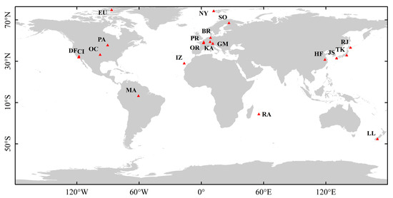
Figure 1.
Locations of the TCCON sites used in this study over the globe.
Table 2.
TCCON sites used in the comparison.
2.4. Cross-Validation Criterion
The XCO2 data from the GOSAT and OCO-2 cannot be directly compared since the spatial resolutions of the GOSAT and OCO-2 are different (Table 1). In nadir, glint, and target modes, the GOSAT footprint can cover from dozens to hundreds of OCO-2 footprints [30]. To compare the datasets, we processed the OCO-2 data based on the time and location of the GOSAT data. We averaged the OCO-2 data over a 10.5 km-diameter circle for each GOSAT footprint, using a temporal criterion of ±1 h. The resulting satellite samples can be considered as observation data of the same place at the same time. This approach yielded a daily XCO2 dataset spanning from September 2014 to May 2016. It is worth noting that, although the algorithms used in the GOSAT and OCO versions of this study differ, we did not account for potential effects resulting from these differences due to the limited scope of our research.
To compare XCO2 measurements from satellites and the TCCON network, we applied geophysical configuration standards that ensure a spatiotemporal separation within ±110 km and ±30 min. This allowed us to choose a set of near-simultaneous data for accurate comparison.
TCCON and GOSAT/OCO-2 XCO2 measurements are subject to various factors, including different a priori profiles and averaging kernels used to describe the sensitivity of the retrieval algorithm to the actual atmospheric state [71,72]. Recent research has demonstrated that the effect of column-averaging kernels on GOSAT and OCO-2 XCO2 is relatively negligible compared to measurement accuracy, making direct comparison applicable in validating satellite’s measurements [36,43]. Zhou et al. [73] did not consider the impact of different averaging kernels of TCCON and GOSAT when accounting for the unavailability of true atmospheric variability. Nonetheless, during the ±2 h when GOSAT passes through the TCCON site located in a low-latitude region with a relatively small solar zenith angle, the average kernels of the GOSAT and TCCON are very similar. Furthermore, Inoue et al. [74] compared the National Institute for Environmental Studies (NIES) SWIR XCO2 retrievals to aircraft data with and without applying GOSAT averaging kernels to the higher-resolution aircraft data, and the differences between aircraft-based XCO2 were evaluated to be less than ±0.4 ppm at most, and less than ±0.1 ppm on average. Similar to previous studies, this research did not consider the influence of different averaging kernels or a priori profiles between remote sounders [36,43,73,74,75].
3. Results
3.1. Data Volume of GOSAT and OCO-2 Observations
To compare the spatial characteristics of the products of the GOSAT and OCO-2 XCO2, this study analyzed XCO2 retrieval data from between September 2014 and May 2016. Figure 2 presents the spatial distribution and data volume of the GOSAT and OCO-2 detections from September 2014 to May 2016, using a grid unit of 2.5 × 2.5 degrees [36]. Within each grid unit, the GOSAT observed yearly data volumes ranging from 0 to 414, while OCO-2 showed a much larger range, from 0 to 2.6 × 10⁴. The GOSAT recorded more data in temperate North America, temperate South America, southern Africa, temperate Asia, and Australia, while OCO-2 had similar results in these regions.
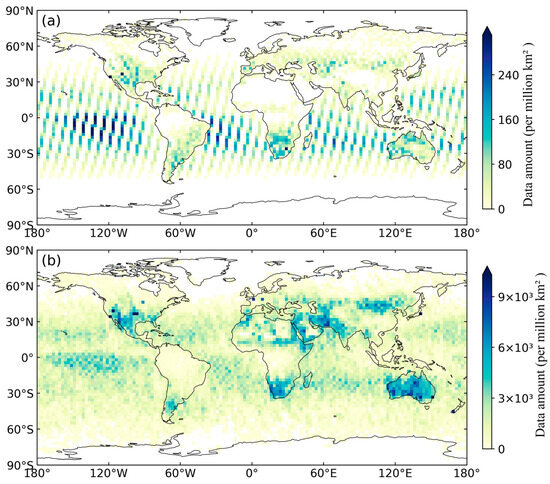
Figure 2.
Data amount in each grid cell (2.5 × 2.5 degrees of grid as a unit) of ACOSXCO2 used in this study ((a), GOSAT; (b), OCO-2).
Figure 3 shows the monthly fluctuations in the data volume per million km2 captured by the GOSAT and OCO-2 during 2015. Both satellites detected the highest amounts of data in Oceania at an average of 44 and 1.3 × 10⁴ monthly data points per million km2, respectively. All other continents displayed the trend of having the largest amount of satellite data during the summer months from June to August and the lowest amounts during the winter months from December to March. One possible explanation for this trend could be the difficulty of retrieving CO2 from space using reflected sunlight, which is affected by factors such as cloud contamination [76], dark surfaces that absorb shortwave infrared wavelengths, and low solar illumination conditions.
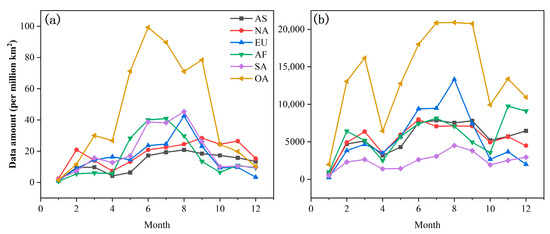
Figure 3.
Monthly variations in data amount across seven continents for (a) GOSAT retrievals, and (b) OCO-2 retrievals in 2015, with AS representing Asia, NA representing North America, EU representing Europe, AF representing Africa, SA representing South America, and OA representing Oceania.
Both satellites show fewer observations in certain regions. For instance, there were fewer observations in Asia, Africa, and North America in April 2015, South America and Europe in October, and Europe and South America in December (Figure 2 and Figure 3). There are two possible reasons for this. Firstly, the ACOS XCO2 inversion algorithm excludes data with a high aerosol optical depth and cloud optical depth, leading to fewer data retrievals in some areas [33,38,76,77]. Secondly, monsoon and pollution events may have reduced the amount of XCO2 data retrieval in some regions [46,78]. Nevertheless, combining the two datasets can provide more comprehensive coverage [43], especially in areas where the two satellites have a low overlap rate.
3.2. Validation of the GOSAT and OCO-2 XCO2 Products Using TCCON Data
This study utilized data products from OCO-2 and the GOSAT XCO2 measurements spanning from September 2014 to May 2016. The TCCON data product (GGG2020) was used for analysis, covering the period from 2004 to 2022. The distribution of the TCCON sites used in this study is shown in Figure 1. Table 2 provides the time range coverage for each TCCON site. The spatiotemporal configuration standards used were ±110 km and ±30 min, as outlined in Section 2.4.
As shown in Figure 4, orthogonal linear regression (OLR) is used instead of ordinary least squares regression (OLS), with TCCON XCO2 as the independent variable and OCO-2 XCO2 as the dependent variable. The motivation behind selecting OLR is that it treats two variables symmetrically when their measurement errors are comparable. However, OLS assumes that the independent variables are measured without error, resulting in relatively smaller slope values compared to OLR estimates, which account for this issue [79]. From Figure 4a,b, it can be seen that, for the GOSAT, the mid-latitude regions of the Northern Hemisphere have the highest number of matched observations. The slope is 0.96, the intercept is 15.03, and the correlation coefficient is 0.85. For OCO-2, the number of matched observations in the mid-latitude regions of the Northern Hemisphere is also the highest, with an intercept of −2.16, a slope of 1.00, and a correlation coefficient of 0.91 (Figure 4b). In Figure 4a,b, the fitting line of OLR is very close to the one-to-one line, indicating that the average difference between the satellite retrieval and TCCON XCO2 is very small. Although OCO-2 has a much larger data volume than the GOSAT (Figure 2 and Figure 3), previous research has indicated that carbon flux inversion results based on OCO-2 observations are not superior to those based on the GOSAT [80,81]. This phenomenon can be attributed to variations in their respective timings and geographical locations. These disparities can introduce distinct influences from atmospheric and surface conditions. For instance, variables like cloud interference, aerosol presence, and surface characteristics can impact the retrieval of XCO2. Moreover, satellite systems are susceptible to sensor malfunctions or performance deterioration during their operational lifespan, posing a potential threat to data quality. Any issues with a satellite’s sensors can compromise the reliability of its data. However, in this study, the correlation coefficient between OCO-2 and the TCCON was higher than that between the GOSAT and TCCON (Figure 4a,b). Generally speaking, although there are errors in the XCO2 values observed by satellites when compared to those of the TCCON, the measured XCO2 values of satellites are usually very consistent with the TCCON data, indicating that satellite products with good quality indicators have been well-calibrated using the TCCON data.
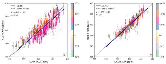
Figure 4.
Scatter plot of the collocations of (a) TCCON and GOSAT XCO2 and (b) TCCON and OCO-2 XCO2 using the ±110 km and ±30 min coincidence criteria. The colors in both panels represent the latitudes of the TCCON sites. The dotted line represents the one-to-one line, and the blue solid line represents the OLR, with the corresponding regression formula shown in the figure. ρ represents the correlation coefficient of the matched data pairs.
Figure 5b,c illustrates the monthly mean XCO2 differences between the TCCON and GOSAT XCO2 (i.e., XCO2 TCCON − XCO2 GOSAT) as well as between the TCCON and OCO-2 XCO2 (i.e., XCO2 TCCON − XCO2 OCO-2) from September 2014 to May 2016. The results indicate that both satellite datasets exhibit good agreement with the TCCON data, with OCO-2 showing slightly better agreement. The mean bias ± standard deviation for the XCO2 differences between the TCCON and GOSAT is 0.92 ± 1.20 ppm, and for the TCCON and OCO-2, it is 0.69 ± 0.97 ppm. These values suggest that the satellite measurements are generally close to the TCCON ground-based observations. This finding is consistent with previous studies: Liang et al. [36] observed differences between GOSAT and TCCON XCO2 that varied over time. After 2014, the overall difference increased, with a mean ± standard deviation of −0.4107 ± 2.216 ppm for the GOSAT and 0.2671 ± 1.56 ppm for OCO-2. Furthermore, they noted that the GOSAT’s monitoring capability has declined in recent years, falling behind OCO-2 in terms of accuracy. Notably, both satellite sources tended to overestimate XCO2 data in the high-value range of approximately 407 ppm and above, especially for OCO-2. Between 390 ppm and 395 ppm, the GOSAT displayed lower XCO2 values compared to the observations of the TCCON. Additionally, O’Dell et al. [34] identified systematic errors in the ACOS XCO2 inversion, which they attributed to inadequate treatment of clouds and aerosols. This highlights the importance of considering and addressing potential sources of error in satellite-based XCO2 measurements.

Figure 5.
Time series of XCO2 measurements from TCCON, GOSAT, and OCO-2 (a) and their inter-comparison differences. Panel (b) shows the difference between TCCON and GOSAT XCO2 measurements (∆XCO2 = TCCON − GOSAT); panel (c) shows the difference between TCCON and OCO-2 XCO2 measurements (∆XCO2 = TCCON − OCO-2); and panel (d) shows the difference between GOSAT and OCO-2 XCO2 measurements (∆XCO2 = GOSAT − OCO-2).
The GOSAT XCO2 data showed the smallest difference of 0.17 ppm in July 2015, while the largest difference was observed in March 2016 at about 3.21 ppm (Figure 5b). Similarly, OCO-2 XCO2 showed the smallest difference of 0.03 ppm in January 2015, while the largest difference was observed in March 2016 at about 1.75 ppm (Figure 5c). It is worth noting that both the GOSAT and OCO-2 displayed the highest data volume during the summer months from June to August, while the lowest data volume was observed during the winter months from December to March (Figure 3). This seasonality in data volume may contribute to the observed differences in XCO2 measurements during specific periods. These findings suggest that the differences between the GOSAT, OCO-2, and TCCON XCO2 increase over time, which is consistent with earlier studies [36,43]. Thus, continual verification of the GOSAT retrieval results is necessary to ensure data quality.
3.3. Comparison of XCO2 Data between GOSAT and OCO-2
To perform a detailed cross-comparison of the GOSAT and OCO-2 XCO2 data, we used the GOSAT satellite site as the standard and screened the OCO-2 XCO2 data based on a distance range of ±10.5 km and a time of ±1 h (see Section 2.4 for details).
In Section 3.2, we have verified the ground observation data of the GOSAT, OCO-2, and TCCON, respectively. The results show that the consistency of the GOSAT and OCO-2 satellite data with the TCCON data is relatively high. Therefore, we performed OLR with the XCO2 data of the GOSAT as the independent variable and the data of OCO-2 as the dependent variable to obtain the scatter plot of the GOSAT and OCO-2 XCO2 (Figure 6). The OLR plot has a slope of 1.02, an intercept of −7.73, and a correlation coefficient of 0.92. The scatter plot is distributed around a one-to-one line, indicating a high correlation between the XCO2 data from the two satellites.
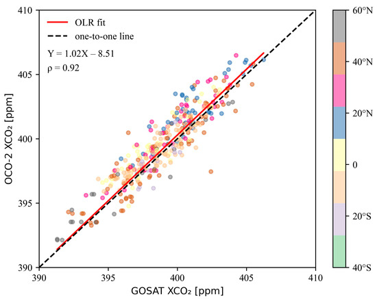
Figure 6.
Scatter plot of the collocations of GOSAT and OCO-2 XCO2 using the ±10.5 km and ±1 h coincidence criteria. The colors represent the latitudes of the satellite sites. The dotted line represents the one-to-one line, and the red solid line represents the orthogonal linear regression (OLR) fit, with the corresponding regression formula shown in the figure. The matched data pairs have a correlation coefficient of ρ.
Figure 5d shows the monthly mean XCO2 difference statistics between the GOSAT and OCO-2 XCO2 (i.e., XCO2 GOSAT − XCO2 OCO−2) from September 2014 to May 2016. The mean bias ± standard deviation of differences is 0.92 ± 1.16 ppm. Overall, the difference between the GOSAT and OCO-2 was the smallest at 0.08 ppm in October 2014, and the largest at approximately 1.51 ppm in April 2016. Figure 5d indicates that there is no apparent time-dependent change in differences, and similar conclusions can be seen in previous studies [30].
By conducting a cross-comparison of the observation results of the GOSAT and OCO-2, we find that the retrieval results of the two satellites are consistent. This shows that the two satellites provide comparable data for understanding the global carbon cycle. Previous studies have also shown good agreement between the GOSAT and OCO-2 XCO2 products, with a correlation coefficient of 0.69 and a standard deviation of −1.0 ppm [45]. The discrepancies in satellite-derived XCO2 data primarily stem from atmospheric conditions. Variations in temperature, pressure, and humidity can significantly impact the absorption and scattering of electromagnetic radiation, which is crucial for estimating carbon dioxide (CO2) concentrations. Apart from atmospheric variables, cloud cover and aerosols also exert influence on satellite-derived XCO2 measurements [76]. These elements tend to lower the signal-to-noise ratio in satellite observations, amplifying measurement uncertainties and introducing perturbations to inversion algorithms. Furthermore, they contribute to scattering and absorption phenomena within the radiative transfer process observed by satellites, ultimately affecting the radiative balance and energy distribution in satellite-derived observations. However, the existence of differences between the two products suggests that there is room for improvement in satellite measurements of XCO2 concentrations. Future research could explore ways to minimize discrepancies between the GOSAT and OCO-2 XCO2 data and improve the accuracy and precision of satellite-based CO2 concentration measurements. It is worth noting that filtering out the lower-quality flag data significantly reduces the amount of matching data, as well as the mean bias and standard deviation [30]. Furthermore, there is no clear time-dependent change in the difference between the retrieval results of the two satellites, indicating that the systematic error between the two satellite configurations is not significant (Figure 5d). Studies suggest that the matching error and retrieval error between satellites could be the main reasons for the deviation between OCO-2 and the GOSAT [43].
3.3.1. Monthly Averaged Time-Series Comparison
In Figure 5a, the time-series variation in XCO2 measurements from the GOSAT and OCO-2 is presented. The two data products exhibit similarities in phase and amplitude, but some differences in magnitude. It can be observed that the GOSAT observations are smaller than the OCO-2 observations. XCO2 measurements by the GOSAT and OCO-2 have consistent seasonal fluctuations and an overall increasing trend.
In general, the concentration of CO2 is typically the highest in spring and winter, and the lowest in summer. This is primarily due to the increased use of heating systems in winter and spring, which rely heavily on fossil fuels such as natural gas, oil, and coal. It is important to note that global statistics reveal significant ffCO2 emissions, totaling 9.836 and 9.844 PgC in 2014 and 2015, respectively [82]. As a result, a large amount of CO2 is emitted into the atmosphere during this time. Furthermore, in winter and spring, plants are in a stage of dormancy and recovery. During this period, strong cellular respiration and weak photosynthesis also result in a significant increase in the CO2 concentration in the atmosphere. The lower temperatures in winter also hinder the decomposition process by inhibiting microbial activity. In late spring, with the onset of warmer temperatures, microbial activity intensifies and decomposition begins. Biomaterials release CO2 in the process. This may be why spring and winter see the highest CO2 concentrations [77]. In this research, however, from May to August, the CO2 concentration shows a decreasing trend. This is because favorable temperatures and precipitation during this period promote vegetation growth, which in turn enhances the photosynthesis process. As a result, the strong presence of plant photosynthesis leads to a decrease in the CO2 concentration. Moreover, we found a lag in XCO2 data from satellite observations. The XCO2 values observed by the GOSAT and OCO-2 peaked in May and June, reaching their lowest values in August and September. There could be two reasons for the lag: firstly, satellites monitor the XCO2 data, and it takes time for the photosynthetic carbon uptake by vegetation on the land surface to influence the upper atmosphere. Hence, there is a time delay in satellite observations compared to ground-level data. Secondly, the calculation of monthly global CO2 concentration trends are likely influenced by the reversed seasons in the northern and southern hemispheres.
We observed some differences in magnitude. The atmospheric CO2 concentrations were higher in each month than in the same month in the previous year (Figure 5a). For example, the XCO2 measurement value of the GOSAT in October 2015 was 398.31 ppm, which was higher than the XCO2 measurement value of the GOSAT in October 2014, which was 395.99 ppm. The primary drivers behind this phenomenon are the release of fossil fuels and other greenhouse gases resulting from human activities, the alteration of land use patterns, and deforestation, also caused by human activities.
Figure 7 presents a comparison of XCO2 concentrations obtained from the GOSAT XCO2 measurements and OCO-2 for six continents, namely Asia, North America, Europe, Africa, South America, and Oceania, from January to December 2015. The time series data from Asia, North America, and Europe, which are mainly located in the Northern Hemisphere, show a significant increasing trend and seasonal fluctuations, with the highest point reached in April and May, and the lowest point in August and September. This trend is primarily influenced by the absorption of CO2 by the terrestrial ecosystem and human-induced CO2 emissions. On the other hand, countries mainly situated in the Southern Hemisphere, such as Africa, South America, and Oceania, do not exhibit this trend, likely due to lower levels of human activities, especially in temperate regions. This conclusion is consistent with previous studies [43,77].
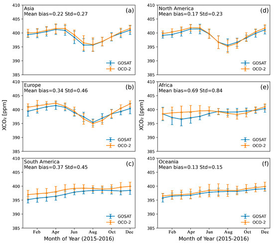
Figure 7.
Spatial distribution of GOSAT XCO2 data from 28 January to 31 December 2015. Comparisons of GOSAT and OCO-2 XCO2 for six continents outlined on the map between 28 January and 31 December 2015 ((a–f) represent Asia, Europe, South America, North America, Africa, and Oceania, respectively.). The error bars represent the standard deviation of the GOSAT and OCO-2 data, respectively.
The GOSAT and OCO-2 were well-consistent in Asia and Oceania, with mean biases and standard deviations of 0.22 ± 0.27 and 0.13 ± 0.15, respectively (Figure 7a,f and Figure 8). To expand on the reasons behind the higher differences in the XCO2 values observed in Asia during May, June, and July (Figure 7a), it is worth noting that the humid climate during this period can significantly impact the accuracy and precision of CO2 column-concentration measurements obtained by the GOSAT and OCO-2 satellites. Clouds and aerosols can greatly affect the accuracy of observations [76]. Additionally, the terrestrial ecosystem in Asia plays a stronger role during these months, contributing to the higher observed differences in XCO2 values. The combined effects of humidity and the role of the ecosystem can lead to an increased variability in measurements, making it challenging to obtain accurate data during this period.
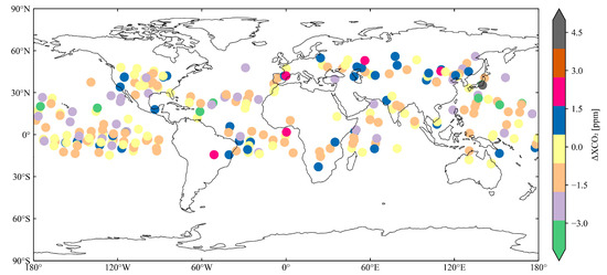
Figure 8.
The spatial variation in the differences between GOSAT and OCO-2.
The months with the largest differences in North America between the GOSAT and OCO-2 data are January, February, and March (Figure 7d), suggesting that these are the months with the greatest variability in CO2 column concentration. Remarkably, South American data exhibit significant differences between the GOSAT and OCO-2 (Figure 7c), primarily due to cloud effects and the impact of the Amazon rainy season on OCO-2 data [83]. The Amazon region is known for its high levels of cloud coverage and rainfall, making it challenging to obtain accurate measurements. During the Amazon rainy season, several factors contribute to the impact on satellite data. The Amazon rainy season typically accompanies the formation of extensive cloud cover, which obscures the line of sight of satellite sensors to the Earth’s surface, resulting in instability and inconsistency in satellite measurements. Additionally, the high-level cloud cover and raindrops in the atmosphere cause optical absorption and scattering effects, interfering with the accuracy of satellite measurements, especially when capturing atmospheric CO2 concentrations. Furthermore, substantial rainfall alters surface humidity and temperature, subsequently affecting the release and absorption processes of CO2 and influencing satellite measurement outcomes. Lastly, the complex terrain in the Amazon region, including rivers and lakes, can also impact satellite measurements, as these topographical features alter the diffusion and transportation patterns of CO2 in the atmosphere. In addition to these factors, sensor settings imposed on satellites can indeed introduce variations in the observed data. These settings affect the sensitivity, resolution, and accuracy of the sensors, impacting their ability to accurately capture and measure atmospheric CO2 concentrations. Consequently, variations in sensor configurations can contribute to the differences observed in satellite-derived XCO2 values across different months and regions. Therefore, these factors contribute to variability in the satellite-derived XCO2 values for the region, making it essential to account for such effects during data processing and analysis.
The XCO2 data for Europe and Africa exhibited poor consistency between the GOSAT and OCO-2 (Figure 7b,e and Figure 8), with mean biases of 0.34 and 0.69, respectively. The largest mean bias occurred in December at 1.65 ppm for Europe and 2.51 ppm in March for Africa, suggesting that certain months may have large uncertainties in the concentration estimates for these regions. Possible contributing factors to this discrepancy include differences in instrument measurement techniques, distinct calculation methods, effects of clouds and atmosphere [76], and surface reflection. In addition, the Congo rainforest is a factor which affects the accuracy of observations from the GOSAT and OCO-2 satellites in Africa. Indeed, the Congo rainforest is a complex and diverse ecosystem in Africa, and its vegetation types and ecosystems may contribute to variability in satellite observations of CO2 column concentrations. Factors such as vegetation growth and rainfall can influence the rates of CO2 absorption and release in the region, further affecting the accuracy and reliability of satellite observation results. Given the complexity of this ecosystem, careful consideration of such natural factors is vital for obtaining accurate and reliable data on CO2 column concentrations in the region.
It is worth noting that there are still some limitations in our study. For instance, we only compared data from the GOSAT and OCO-2 satellites during a specific period, and the results may not be representative of the long-term differences between the two datasets. Additionally, the analysis of factors affecting the differences between the GOSAT and OCO-2 data could be further improved by considering more detailed meteorological and atmospheric conditions. Nevertheless, our study provides important insights into the complementarity of the GOSAT and OCO-2 data and contributes to a better understanding of global carbon cycling and climate change.
3.3.2. Seasonal Climatology Comparison
The distribution of XCO2 in the atmosphere exhibits significant latitudinal variation, and we conducted a study to calculate its latitudinal gradient using data from global GOSAT and OCO-2 footprint observations. Figure 9 displays the seasonal mean XCO2 concentration distributions for the GOSAT and OCO-2 satellites from spring to winter in 2015. The OCO-2 satellite has collected considerably more data than the GOSAT, and both satellites show periodic fluctuations in the monthly average concentrations of XCO2 across changing seasons. The spatiotemporal distribution of the GOSAT and OCO-2 data is largely consistent.
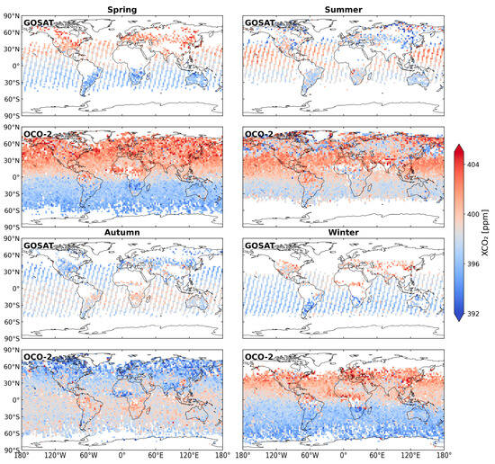
Figure 9.
Spatial Distribution of XCO2 in different seasons as observed by GOSAT and OCO-2 for the year 2015; spring refers to March–May, summer to June–August, autumn to September–November, and winter to December–February.
Figure 10 presents the latitudinal variations in XCO2, as captured by the GOSAT and OCO-2 during various seasons, spanning 45°S–50°N at 5° latitude intervals. This broad latitude range encompasses diverse regions, including South America, North America, Africa, Asia, and Oceania. Notable countries within this range include Brazil and Argentina in South America, the United States in North America, Egypt in Africa, and India and China in Asia. Additionally, Oceania is represented by countries such as Australia and New Zealand. In 2015, both satellites reflected seasonal and latitudinal variations in their observations.
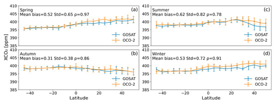
Figure 10.
Latitudinal variation trend of XCO2 in GOSAT and OCO-2 (45°S–50°N, with latitude intervals of 5°); (a) spring refers to March–May, (b) summer to June–August, (c) autumn to September–November, and (d) winter to December–February.
During spring, the XCO2 correlation between the GOSAT and OCO-2 was highly consistent, with a correlation coefficient of 0.97 (Figure 10a). The latitudinal gradient indicated that XCO2 was lower in the Southern Hemisphere than in the corresponding latitudes in the Northern Hemisphere. This could be attributed to plants entering a recovery phase, during which respiration is higher than photosynthesis, leading to an increase in the atmospheric CO2 concentration [84]. The maximum deviation occurs in the latitude range from 10 to 30°N, with an average error of 1.54 ppm.
In summer, the correlation between the GOSAT and OCO-2 was the lowest (correlation coefficient of 0.78), with a mean bias ± standard deviation of differences of 0.62 ± 0.82 ppm (Figure 10c). One potential reason for this disparity could be the effect of cloud cover and aerosol changes [76], which may have hampered the accuracy of both satellites’ observations. Notably, the XCO2 in the Northern Hemisphere showed a significant decrease, driven primarily by strong CO2 absorption due to vegetation photosynthesis during the season. The lower concentration of XCO2 in summer is because higher temperatures and radiation promote the assimilation of atmospheric CO2 during the day and respiration at night, and green plants such as rice and forests absorb atmospheric CO2 through photosynthesis during this period [85]. The maximum deviation occurs between the latitude range of 40–50°N, with an error of 2.44 ppm between latitudes.
As the season turned to fall, the XCO2 correlation between the two satellites was 0.86 (Figure 10b), and the latitudinal gradient demonstrated a remarkable shift from that observed during spring. In fall, XCO2 in the southern hemisphere was higher than that measured in the corresponding latitudes in the Northern Hemisphere, reflecting variations in the patterns of anthropogenic emissions and other CO2 sources.
In winter, constraints to the GOSAT data captured high-latitude areas in the Northern Hemisphere due to issues such as cloud cover and the solar zenith angle (Figure 10d). Concentrations of XCO2 are always higher in the Northern Hemisphere, possibly due to the large amount of biomass burning that occurs during this period. Also, anthropogenic emissions, such as winter heating, emit a large amount of CO2 in the Northern Hemisphere during winter, and natural absorption is weakened [86,87]. These factors have greatly increased the amount of CO2 in the atmosphere [88,89,90]. The maximum deviation occurs in the latitude range of 30–45°N, with an error of 1.76 ppm between latitudes. Despite these constraints, however, satellite observations afforded real-time and objective measurements of atmospheric CO2 concentrations, providing a window into the spatial shifts and variations in atmospheric CO2 concentrations attributable to anthropogenic emissions and other sources. Overall, these findings provide important insights into the complex dynamics of CO2 in the atmosphere and highlight the need for the continued monitoring of global CO2 levels to better understand and address the effects of climate change.
One significant factor contributing to the seasonal fluctuations in the measurements of XCO2 from the GOSAT and OCO-2 is the Asian monsoon climate, which has a crucial impact on the concentration of CO2 [91] and, therefore, affects global CO2 changes. The Asian monsoon can be divided into two types: the southwest monsoon and the east-Asian monsoon [92]. The southwest monsoon is prevalent during the summer months in South Asia and Southeast Asia, and the Indian summer monsoon is its typical representative. It originates from the southeast trade wind on the Indian Ocean, and after crossing the equator, it is affected by the earth’s rotation and turns southwest, mainly affecting the Indian subcontinent. The East-Asian monsoon is a crucial part of the Asian monsoon, and its changes affect the weather and climate. The East-Asian near-surface monsoon is the second-most prominent after the South-Asian and Southeast-Asian summer monsoons, and it affects eastern China, the Korean Peninsula, and Japan. In most areas of Asia, from March to May is considered pre-monsoon, from June to September is considered monsoon, and from October to November is considered post-monsoon [91].
Research conducted by Mustafa et al. [84] indicates that the CO2 concentration is the highest in the pre-monsoon period and the lowest during the monsoon period, with similar findings obtained in this study (Figure 5 and Figure 7). Research results from An et al. [90] suggest that the atmospheric CO2 concentration being the highest during the pre-monsoon period can be attributed to (1) a large amount of biomass burning [88,89], (2) low wind-speed in the pre-monsoon period leading to the accumulation of atmospheric CO2 [93], and (3) higher temperature and radiation during the summer, stimulating atmospheric CO2 absorption during the day and respiration at night [85]. Sreenivas et al. [89] analyze the time series of atmospheric CO2 concentrations in Oman and show similar results to the decrease in atmospheric CO2 concentrations during the monsoon season. The emergence of the summer monsoon season is the primary source of precipitation in some areas; therefore an essential factor controlling vegetation in these areas. During the rainy season, soil moisture increases, thereby enhancing the photosynthetic process and ultimately reducing the CO2 in the atmosphere [94]. Figure 5 and Figure 7 show that, after the monsoon period (October–November), atmospheric CO2 levels begin to increase again. This increase is likely due to the excess CO2 produced by fossil fuel consumption, which is emitted into the atmosphere [95].
4. Summary and Conclusions
The GOSAT and OCO-2 are the first two satellite missions dedicated to monitoring global CO2 distribution. It is of significant importance to compare and analyze the differences between these two products. In this study, we carried out a detailed comparison between the GOSAT and OCO-2 satellite data spanning from September 2014 to May 2016.
Firstly, we conducted a comparative analysis of the spatial characteristics of XCO2 products from the GOSAT and OCO-2 satellites using data collected between September 2014 and May 2016. Our findings revealed significant differences in data volume within each 2.5 × 2.5-degree grid cell. Specifically, the GOSAT’s annual data volume ranged from 0 to 414, whereas OCO-2 exhibited a much wider range, from 0 to 2.6 × 10⁴. Notably, in the Oceania region, both satellites captured the highest volume of data, averaging 44 and 1.3 × 10⁴ data points per million km2 per month, respectively. When comparing data volumes among continents, we observed that the highest amount of satellite data was obtained during the summer months (June–August) and the lowest was obtained in winter (December–February). These findings highlight the challenges associated with obtaining accurate data from space. Factors such as cloud pollution, surface reflections, and low solar illumination can impede data collection efforts. Consequently, further advancements are necessary to overcome these limitations and improve the reliability of spaceborne CO2 data.
Secondly, we conducted a verification of the GOSAT and OCO-2 XCO2 inversion products using ground-based TCCON measurements. The satellite XCO2 measurements were found to be generally consistent with the TCCON data. Specifically, for the GOSAT, the mean bias ± standard deviation was 0.92 ± 1.20 ppm, and the correlation coefficient was 0.85. Similarly, for OCO-2, the mean bias ± standard deviation was 0.69 ± 0.97 ppm, with a correlation coefficient of 0.91. It is worth noting that the agreement between the TCCON and OCO-2 was better than that of the GOSAT. However, it is important to highlight that the fitted lines of the OLR for both satellites and the TCCON are closely aligned with the one-to-one line. This implies that the average difference between the satellite retrieval and the TCCON XCO2 values was minimal. Additionally, our analysis revealed that the disparities between the GOSAT, OCO-2, and TCCON XCO2 values showed an increasing trend over time. Therefore, it is crucial to continuously validate future data searches to ensure high data quality [43,81].
Finally, we performed a detailed cross-comparison of the GOSAT and OCO-2 XCO2 data after validating their datasets to assess their consistency. The analysis revealed a high correlation between the two satellite datasets. The mean bias and standard deviation of XCO2 observations for the GOSAT and OCO-2 were 0.92 ± 1.16, and the correlation coefficient was 0.92, indicating a strong relationship between the XCO2 data obtained from both satellites. In Asia and Oceania, the data from the GOSAT and OCO-2 exhibited remarkable consistency, with mean deviations and standard deviations of 0.22 ± 0.27 and 0.13 ± 0.15, respectively (Figure 7a,f and Figure 8). The North American region showed the best agreement, with a mean deviation and standard deviation of 0.17 ± 0.23 ppm (Figure 7d). However, in South America, significant differences were observed (Figure 7c), primarily due to cloud effects and the impact of the Amazon rainy season on OCO-2 data. The mean bias and standard deviation for South America were 0.37 ± 0.45. Unfortunately, the data from Europe and Africa exhibited poor agreement between the GOSAT and OCO-2 (Figure 7b,e and Figure 8), with mean deviations of 0.34 and 0.69, respectively. When considering seasonal climatology, spring showed the highest XCO2 correlation between the GOSAT and OCO-2, with a correlation coefficient of 0.97 (Figure 10a). However, the correlation decreased in summer (correlation coefficient of 0.78, Figure 10c). In autumn, the XCO2 correlation between the two satellites was 0.86 (Figure 10b), and the latitudinal gradient differed significantly from that observed in spring. During winter, several factors can affect the quality of XCO2 data, including cloud cover and the sun’s zenith angle. In Asia, CO2 concentrations were notably influenced by the monsoon climate, resulting in higher XCO2 levels during the pre-monsoon period and lower levels during the monsoon.
Overall, while the GOSAT and OCO-2 XCO2 data exhibited a high correlation, discrepancies were noted in certain regions and seasons. Factors such as cloud effects, seasonal variations, and regional climate patterns contributed to the observed differences. Further research and advancements are necessary to enhance the agreement and reliability of XCO2 data between these satellites.
The spatial variation information obtained through satellite observations provides valuable insights into the concentration patterns of CO2, offering crucial information for understanding the impacts of climate change. As two greenhouse gas monitoring satellites in orbit, the GOSAT and OCO-2 possess the capability to detect atmospheric CO2. In this study, we compared the XCO2 inversion results of the GOSAT and OCO-2 and found that they exhibit good consistency but still show some differences. Although some differences exist among the datasets, the overall findings demonstrate a strong correlation between the satellite measurements of XCO2. These results emphasize the importance of continued monitoring and calibration efforts to ensure the accurate assessment and understanding of atmospheric CO2 levels. Our study reinforces our confidence in the reliability of satellite-derived XCO2 measurements, particularly in regions like Asia, North America, and Oceania. The observed seasonal variations and their causes highlight the need for targeted research during specific periods, such as summer, to address challenges like cloud cover and aerosol interference. This understanding will guide future data collection and processing strategies. In future works, we will analyze more XCO2 products at different spatiotemporal resolutions with the increase in different available satellite and model simulation data. Furthermore, we will conduct a more extended analysis spanning several decades to investigate long-term trends in XCO2 concentrations. Understanding how these trends evolve over time is critical for assessing the effectiveness of climate policies and mitigation strategies.
Author Contributions
Conceptualization, J.Z., H.Z. and S.Z.; Formal analysis, J.Z.; Funding acquisition, H.Z. and S.Z.; Investigation, J.Z. and S.Z.; Methodology, J.Z. and S.Z.; Project administration, H.Z. and S.Z.; Resources, J.Z. and H.Z.; Software, J.Z., H.Z. and S.Z.; Supervision, H.Z. and S.Z.; Validation, J.Z.; Visualization, J.Z.; Writing—original draft, J.Z. and S.Z.; Writing—review & editing, J.Z., H.Z. and S.Z. All authors have read and agreed to the published version of the manuscript.
Funding
This research was funded by the National Natural Science Foundation of China (Grant No. 41890854), the Innovation Project of LREIS (Grant No. KPI005) and Chinese Academy of Sciences Class A Strategic Pilot Science and Technology Project (XDA23100202).
Data Availability Statement
Data are available upon request due to restrictions.
Conflicts of Interest
The authors declare no conflict of interest.
References
- Mak, H.W.L.; Ng, D.C.Y. Spatial and Socio-Classification of Traffic Pollutant Emissions and Associated Mortality Rates in High-Density Hong Kong via Improved Data Analytic Approaches. Int. J. Environ. Res. Public Health 2021, 18, 6532. [Google Scholar] [CrossRef] [PubMed]
- Mohsin, M.; Naseem, S.; Sarfraz, M.; Azam, T. Assessing the effects of fuel energy consumption, foreign direct investment and GDP on CO2 emission: New data science evidence from Europe & Central Asia. Fuel 2022, 314, 123098. [Google Scholar]
- Yarzábal, L.A.; Salazar, L.M.B.; Batista-García, R.A. Climate change, melting cryosphere and frozen pathogens: Should we worry…? Environ. Sustain. 2021, 4, 489–501. [Google Scholar] [CrossRef]
- Deng, S.; Jalaludin, B.B.; Antó, J.M.; Hess, J.J.; Huang, C. Climate change, air pollution, and allergic respiratory diseases: A call to action for health professionals. Chin. Med. J. 2020, 133, 1552–1560. [Google Scholar] [CrossRef] [PubMed]
- Amirkhani, M.; Ghaemimood, S.; von Schreeb, J.; El-Khatib, Z.; Yaya, S. Extreme weather events and death based on temperature and CO2 emission—A global retrospective study in 77 low-, middle- and high-income countries from 1999 to 2018. Prev. Med. Rep. 2022, 28, 101846. [Google Scholar] [CrossRef] [PubMed]
- Clarke, B.J.; Otto, F.E.; Jones, R.G. Inventories of extreme weather events and impacts: Implications for loss and damage from and adaptation to climate extremes. Clim. Risk Manag. 2021, 32, 100285. [Google Scholar] [CrossRef]
- IPCC. Climate Change 2014: Synthesis Report. In Contribution of Working Groups I, II and III to the Fifth Assessment Report of the Intergovernmental Panel on Climate Change; IPCC: Geneva, Switzerland, 2014; p. 151. [Google Scholar]
- Raza, A.; Razzaq, A.; Mehmood, S.; Zou, X.; Zhang, X.; Lv, Y.; Xu, J. Impact of Climate Change on Crops Adaptation and Strategies to Tackle Its Outcome: A Review. Plants 2019, 8, 34. [Google Scholar] [CrossRef] [PubMed]
- Houghton, R.A. Balancing the global carbon budget. Annu. Rev. Earth Planet. Sci. 2007, 35, 313–347. [Google Scholar] [CrossRef]
- Solomon, S.; Qin, D.; Manning, M.; Chen, Z.; Marquis, M.; Averyt, K.B.; Tignor, M.; Miller, H.L. Contribution of Working Group I to the Fourth Assessment Report of the Intergovernmental Panel on Climate Change; Cambridge University Press: Cambridge, UK, 2007. [Google Scholar]
- IPCC. Summary for Policymakers. In Climate Change 2022—Mitigation of Climate Change: Working Group III Contribution to the Sixth Assessment Report of the Intergovernmental Panel on Climate Change; Cambridge University Press: Cambridge, UK, 2023; pp. 3–48. [Google Scholar]
- Zhou, Y.; Smith, S.J.; Zhao, K.; Imhoff, M.; Thomson, A.; Bond-Lamberty, B.; Asrar, G.R.; Zhang, X.; He, C.; Elvidge, C.D. A global map of urban extent from nightlights. Environ. Res. Lett. 2015, 10, 54011. [Google Scholar] [CrossRef]
- Seto, K.C.; Dhakal, S.; Bigio, A.; Blanco, H.; Carlo Delgado, G.; Dewar, D.; Huang, L.; Inaba, A.; Kansal, A.; Lwasa, S. Human Settlements, Infrastructure, and Spatial Planning; UCLA: Los Angeles, CA, USA, 2014. [Google Scholar]
- Le Quéré, C.; Peters, G.P.; Friedlingstein, P.; Andrew, R.M.; Canadell, J.G.; Davis, S.J.; Jackson, R.B.; Jones, M.W. Fossil CO2 emissions in the post-COVID-19 era. Nat. Clim. Chang. 2021, 11, 197–199. [Google Scholar] [CrossRef]
- Yañez, C.C.; Hopkins, F.M.; Xu, X.; Tavares, J.F.; Welch, A.; Czimczik, C.I. Reductions in California’s Urban Fossil Fuel CO2 Emissions During the COVID-19 Pandemic. Agu Adv. 2022, 3, e2022AV000732. [Google Scholar] [CrossRef]
- Vandyck, T.; Keramidas, K.; Saveyn, B.; Kitous, A.; Vrontisi, Z. A global stocktake of the Paris pledges: Implications for energy systems and economy. Glob. Environ. Change 2016, 41, 46–63. [Google Scholar] [CrossRef]
- Labzovskii, L.D.; Mak, H.W.L.; Takele Kenea, S.; Rhee, J.; Lashkari, A.; Li, S.; Goo, T.; Oh, Y.; Byun, Y. What can we learn about effectiveness of carbon reduction policies from interannual variability of fossil fuel CO2 emissions in East Asia? Environ. Sci. Policy 2019, 96, 132–140. [Google Scholar] [CrossRef]
- Eisenack, K.; Hagen, A.; Mendelevitch, R.; Vogt, A. Politics, profits and climate policies: How much is at stake for fossil fuel producers? Energy Res. Soc. Sci. 2021, 77, 102092. [Google Scholar] [CrossRef]
- Liu, Y.; Wang, J.; Che, K.; Cai, Z.; Yang, D.; Wu, L. Satellite remote sensing of greenhouse gases: Progress and trends. Natl. Remote Sens. Bull. 2021, 25, 53–64. [Google Scholar] [CrossRef]
- Chevallier, F.; Bréon, F.; Rayner, P.J. Contribution of the Orbiting Carbon Observatory to the estimation of CO2 sources and sinks: Theoretical study in a variational data assimilation framework. J. Geophys. Res. 2007, 112, D09307. [Google Scholar] [CrossRef]
- Schneising, O.; Buchwitz, M.; Burrows, J.P.; Bovensmann, H.; Reuter, M.; Notholt, J.; Macatangay, R.; Warneke, T. Three years of greenhouse gas column-averaged dry air mole fractions retrieved from satellite–Part 1: Carbon dioxide. Atmos. Chem. Phys. 2008, 8, 3827–3853. [Google Scholar] [CrossRef]
- Hungershoefer, K.; Breon, F.; Peylin, P.; Chevallier, F.; Rayner, P.; Klonecki, A.; Houweling, S.; Marshall, J. Evaluation of various observing systems for the global monitoring of CO2 surface fluxes. Atmos. Chem. Phys. 2010, 10, 10503–10520. [Google Scholar] [CrossRef]
- Reuter, M.; Bovensmann, H.; Buchwitz, M.; Burrows, J.P.; Connor, B.J.; Deutscher, N.M.; Griffith, D.W.T.; Heymann, J.; Keppel-Aleks, G.; Messerschmidt, J.; et al. Retrieval of atmospheric CO2 with enhanced accuracy and precision from SCIAMACHY: Validation with FTS measurements and comparison with model results. J. Geophys. Res. 2011, 116, D04301. [Google Scholar]
- Lei, L.; Guan, X.; Zeng, Z.; Zhang, B.; Ru, F.; Bu, R. A comparison of atmospheric CO2 concentration GOSAT-based observations and model simulations. Sci. China Earth Sci. 2014, 57, 1393–1402. [Google Scholar] [CrossRef]
- Zeng, N.; Zhao, F.; Collatz, G.J.; Kalnay, E.; Salawitch, R.J.; West, T.O.; Guanter, L. Agricultural Green Revolution as a driver of increasing atmospheric CO2 seasonal amplitude. Nature 2014, 515, 394–397. [Google Scholar] [CrossRef] [PubMed]
- Deng, F.; Jones, D.B.A.; Henze, D.K.; Bousserez, N.; Bowman, K.W.; Fisher, J.B.; Nassar, R.; O’Dell, C.; Wunch, D.; Wennberg, P.O.; et al. Inferring regional sources and sinks of atmospheric CO2 from GOSAT XCO2 data. Atmos. Chem. Phys. 2014, 14, 3703–3727. [Google Scholar] [CrossRef]
- Sheng, M.; Lei, L.; Zeng, Z.; Rao, W.; Zhang, S. Detecting the Responses of CO2 Column Abundances to Anthropogenic Emissions from Satellite Observations of GOSAT and OCO-2. Remote Sens. 2021, 13, 3524. [Google Scholar] [CrossRef]
- Zhang, Y.; Liu, X.; Lei, L.; Liu, L. Estimating Global Anthropogenic CO2 Gridded Emissions Using a Data-Driven Stacked Random Forest Regression Model. Remote Sens. 2022, 14, 3899. [Google Scholar] [CrossRef]
- Mustafa, F.; Bu, L.; Wang, Q.; Yao, N.; Shahzaman, M.; Bilal, M.; Aslam, R.W.; Iqbal, R. Neural-network-based estimation of regional-scale anthropogenic CO2 emissions using an Orbiting Carbon Observatory-2 (OCO-2) dataset over East and West Asia. Atmos. Meas. Tech. 2021, 14, 7277–7290. [Google Scholar] [CrossRef]
- Kataoka, F.; Crisp, D.; Taylor, T.; O’Dell, C.; Kuze, A.; Shiomi, K.; Suto, H.; Bruegge, C.; Schwandner, F.; Rosenberg, R.; et al. The Cross-Calibration of Spectral Radiances and Cross-Validation of CO2 Estimates from GOSAT and OCO-2. Remote Sens. 2017, 9, 1158. [Google Scholar] [CrossRef]
- Kulawik, S.; Wunch, D.; O’Dell, C.; Frankenberg, C.; Reuter, M.; Oda, T.; Chevallier, F.; Sherlock, V.; Buchwitz, M.; Osterman, G.; et al. Consistent evaluation of ACOS-GOSAT, BESD-SCIAMACHY, CarbonTracker, and MACC through comparisons to TCCON. Atmos. Meas. Tech. 2016, 9, 683–709. [Google Scholar] [CrossRef]
- Jung, Y.; Kim, J.; Kim, W.; Boesch, H.; Lee, H.; Cho, C.; Goo, T. Impact of Aerosol Property on the Accuracy of a CO2 Retrieval Algorithm from Satellite Remote Sensing. Remote Sens. 2016, 8, 322. [Google Scholar] [CrossRef]
- O’Dell, C.W.; Connor, B.; Bösch, H.; O’Brien, D.; Frankenberg, C.; Castano, R.; Christi, M.; Eldering, D.; Fisher, B.; Gunson, M.; et al. The ACOS CO2 retrieval algorithm—Part 1: Description and validation against synthetic observations. Atmos. Meas. Tech. 2012, 5, 99–121. [Google Scholar] [CrossRef]
- O’Dell, C.W.; Eldering, A.; Wennberg, P.O.; Crisp, D.; Gunson, M.R.; Fisher, B.; Frankenberg, C.; Kiel, M.; Lindqvist, H.; Mandrake, L.; et al. Improved retrievals of carbon dioxide from Orbiting Carbon Observatory-2 with the version 8 ACOS algorithm. Atmos. Meas. Tech. 2018, 11, 6539–6576. [Google Scholar] [CrossRef]
- Wunch, D.; Wennberg, P.O.; Osterman, G.; Fisher, B.; Naylor, B.; Roehl, C.M.; O’Dell, C.; Mandrake, L.; Viatte, C.; Kiel, M.; et al. Comparisons of the Orbiting Carbon Observatory-2 (OCO-2) XCO2 measurements with TCCON. Atmos. Meas. Tech. 2017, 10, 2209–2238. [Google Scholar] [CrossRef]
- Liang, A.; Gong, W.; Han, G.; Xiang, C. Comparison of Satellite-Observed XCO2 from GOSAT, OCO-2, and Ground-Based TCCON. Remote Sens. 2017, 9, 1033. [Google Scholar] [CrossRef]
- Bie, N.; Lei, L.; Zeng, Z.; Cai, B.; Yang, S.; He, Z.; Wu, C.; Nassar, R. Regional uncertainty of GOSAT XCO2 retrievals in China: Quantification and attribution. Atmos. Meas. Tech. 2018, 11, 1251–1272. [Google Scholar] [CrossRef]
- Crisp, D.; Fisher, B.M.; O’Dell, C.; Frankenberg, C.; Basilio, R.; Bösch, H.; Brown, L.R.; Castano, R.; Connor, B.; Deutscher, N.M. The ACOS CO2 retrieval algorithm–part II: Global X CO2 data characterization. Atmos. Meas. Tech. 2012, 5, 687–707. [Google Scholar] [CrossRef]
- Zhang, L.L.; Yue, T.X.; Wilson, J.P.; Zhao, N.; Zhao, Y.P.; Du, Z.P.; Liu, Y. A comparison of satellite observations with the XCO2 surface obtained by fusing TCCON measurements and GEOS-Chem model outputs. Sci. Total Environ. 2017, 601–602, 1575–1590. [Google Scholar] [CrossRef] [PubMed]
- Karbasi, S.; Malakooti, H.; Rahnama, M.; Azadi, M. Study of mid-latitude retrieval XCO2 greenhouse gas: Validation of satellite-based shortwave infrared spectroscopy with ground-based TCCON observations. Sci. Total Environ. 2022, 836, 155513. [Google Scholar] [CrossRef] [PubMed]
- Hong, X.; Zhang, P.; Bi, Y.; Liu, C.; Sun, Y.; Wang, W.; Chen, Z.; Yin, H.; Zhang, C.; Tian, Y.; et al. Retrieval of Global Carbon Dioxide from TanSat Satellite and Comprehensive Validation with TCCON Measurements and Satellite Observations. IEEE Trans. Geosci. Remote Sens. 2022, 60, 1–16. [Google Scholar] [CrossRef]
- Chen, Y.; Cheng, J.; Song, X.; Liu, S.; Sun, Y.; Yu, D.; Fang, S. Global-Scale Evaluation of XCO2 Products from GOSAT, OCO-2 and CarbonTracker Using Direct Comparison and Triple Collocation Method. Remote Sens. 2022, 14, 5635. [Google Scholar] [CrossRef]
- Kong, Y.; Chen, B.; Measho, S. Spatio-Temporal Consistency Evaluation of XCO2 Retrievals from GOSAT and OCO-2 Based on TCCON and Model Data for Joint Utilization in Carbon Cycle Research. Atmosphere 2019, 10, 354. [Google Scholar] [CrossRef]
- Yokota, T.; Yoshida, Y.; Eguchi, N.; Ota, Y.; Tanaka, T.; Watanabe, H.; Maksyutov, S. Global concentrations of CO2 and CH4 retrieved from GOSAT: First preliminary results. Sola 2009, 5, 160–163. [Google Scholar] [CrossRef]
- Jing, Y.; Shi, J.; Zhang, P.; Wang, T.; Chen, L. Comparison of atmospheric carbon dioxide concentration based on GOSAT and OCO-2 observations. In Proceedings of the 2016 IEEE International Geoscience and Remote Sensing Symposium, Beijing, China, 10–15 July 2016; pp. 4071–4073. [Google Scholar]
- Kort, E.A.; Frankenberg, C.; Miller, C.E.; Oda, T. Space-based observations of megacity carbon dioxide. Geophys. Res. Lett. 2012, 39, L17806. [Google Scholar] [CrossRef]
- Kuze, A.; Urabe, T.; Suto, H.; Kaneko, Y.; Hamazaki, T. The instrumentation and the BBM test results of thermal and near-infrared sensor for carbon observation (TANSO) on GOSAT. Infrared Spaceborne Remote Sens. XIV SPIE 2006, 6297, 138–145. [Google Scholar]
- Boland, S.; Bösch, H.; Brown, L.; Burrows, J.; Ciais, P.; Connor, B.; Crisp, D.; Denning, S.; Doney, S.; Engelen, R. The Need for Atmospheric Carbon Dioxide Measurements from Space: Contributions from a Rapid Reflight of the Orbiting Carbon Observatory; Jet Propulsion Laboratory: La Cañada, CA, USA, 2009. [Google Scholar]
- Crisp, D.; Pollock, H.R.; Rosenberg, R.; Chapsky, L.; Lee, R.A.M.; Oyafuso, F.A.; Frankenberg, C.; O’Dell, C.W.; Bruegge, C.J.; Doran, G.B.; et al. The on-orbit performance of the Orbiting Carbon Observatory-2 (OCO-2) instrument and its radiometrically calibrated products. Atmos. Meas. Tech. 2017, 10, 59–81. [Google Scholar] [CrossRef]
- Wunch, D.; Toon, G.C.; Blavier, J.L.; Washenfelder, R.A.; Notholt, J.; Connor, B.J.; Griffith, D.W.T.; Sherlock, V.; Wennberg, P.O. The Total Carbon Column Observing Network. Philos. Trans. R. Soc. A Math. Phys. Eng. Sci. 2011, 369, 2087–2112. [Google Scholar] [CrossRef] [PubMed]
- Notholt, J.; Petri, C.; Warneke, T.; Buschmann, M. TCCON Data from Bremen (DE), Release GGG2020R0; TCCON data archive, hosted by CaltechDATA; California Institute of Technology: Pasadena, CA, USA, 2022. [Google Scholar]
- Wennberg, P.O.; Roehl, C.M.; Wunch, D.; Blavier, J.F.; Toon, G.C.; Allen, N.T.; Treffers, R.; Laughner, J. TCCON Data from Caltech (US), Release GGG2020R0; TCCON data archive, hosted by CaltechDATA; California Institute of Technology: Pasadena, CA, USA, 2022. [Google Scholar]
- Iraci, L.T.; Podolske, J.R.; Roehl, C.; Wennberg, P.O.; Blavier, J.F.; Allen, N.; Wunch, D.; Osterman, G.B. TCCON Data from Edwards (US), Release GGG2020R0; TCCON data archive, hosted by CaltechDATA; California Institute of Technology: Pasadena, CA, USA, 2022. [Google Scholar]
- Strong, K.; Roche, S.; Franklin, J.E.; Mendonca, J.; Lutsch, E.; Weaver, D.; Fogal, P.F.; Drummond, J.R.; Batchelor, R.; Lindenmaier, R. TCCON Data from Eureka (CA), Release GGG2020R0; TCCON data archive, hosted by CaltechDATA; California Institute of Technology: Pasadena, CA, USA, 2022. [Google Scholar]
- Sussmann, R.; Rettinger, M. TCCON Data from Garmisch (DE), Release GGG2020R0; TCCON data archive, hosted by CaltechDATA; California Institute of Technology: Pasadena, CA, USA, 2023. [Google Scholar]
- Liu, C.; Wang, W.; Sun, Y.; Shan, C. TCCON Data from Hefei (PRC), Release GGG2020R0; TCCON data archive, hosted by CaltechDATA; California Institute of Technology: Pasadena, CA, USA, 2022. [Google Scholar]
- García, O.E.; Schneider, M.; Herkommer, B.; Gross, J.; Hase, F.; Blumenstock, T.; Sepúlveda, E. TCCON Data from Izana (ES), Release GGG2020R1; TCCON data archive, hosted by CaltechDATA; California Institute of Technology: Pasadena, CA, USA, 2022. [Google Scholar]
- Shiomi, K.; Kawakami, S.; Ohyama, H.; Arai, K.; Okumura, H.; Ikegami, H.; Usami, M. TCCON Data from Saga (JP), Release GGG2020R0; TCCON data archive, hosted by CaltechDATA; California Institute of Technology: Pasadena, CA, USA, 2022. [Google Scholar]
- Hase, F.; Herkommer, B.; Groß, J.; Blumenstock, T.; Kiel, M.Ä.; Dohe, S. TCCON Data from Karlsruhe (DE), Release GGG2020R1; TCCON data archive, hosted by CaltechDATA; California Institute of Technology: Pasadena, CA, USA, 2023. [Google Scholar]
- Sherlock, V.; Connor, B.; Robinson, J.; Shiona, H.; Smale, D.; Pollard, D.F. TCCON Data from Lauder (NZ), 125HR, Release GGG2020R0; TCCON data archive, hosted by CaltechDATA; California Institute of Technology: Pasadena, CA, USA, 2022. [Google Scholar]
- Dubey, M.K.; Henderson, B.G.; Allen, N.T.; Blavier, J.F.; Roehl, C.M.; Wunch, D. TCCON Data from Manaus (BR), Release GGG2020R0; TCCON data archive, hosted by CaltechDATA; California Institute of Technology: Pasadena, CA, USA, 2022. [Google Scholar]
- Buschmann, M.; Petri, C.; Palm, M.; Warneke, T.; Notholt, J. TCCON Data from Ny-Ålesund, Svalbard (NO), Release GGG2020R0; TCCON data archive, hosted by CaltechDATA; California Institute of Technology: Pasadena, CA, USA, 2022. [Google Scholar]
- Wennberg, P.O.; Wunch, D.; Roehl, C.M.; Blavier, J.F.; Toon, G.C.; Allen, N.T. TCCON Data from Lamont (US), Release GGG2020R0; TCCON data archive, hosted by CaltechDATA; California Institute of Technology: Pasadena, CA, USA, 2022. [Google Scholar]
- Warneke, T.; Petri, C.; Notholt, J.; Buschmann, M. TCCON Data from Orléans (FR), Release GGG2020R0; TCCON data archive, hosted by CaltechDATA; California Institute of Technology: Pasadena, CA, USA, 2022. [Google Scholar]
- Wennberg, P.O.; Roehl, C.M.; Wunch, D.; Toon, G.C.; Blavier, J.F.; Washenfelder, R.; Keppel-Aleks, G.; Allen, N.T. TCCON Data from Park Falls (US), Release GGG2020R1; TCCON data archive, hosted by CaltechDATA; California Institute of Technology: Pasadena, CA, USA, 2022. [Google Scholar]
- Té, Y.; Jeseck, P.; Janssen, C. TCCON Data from Paris (FR), Release GGG2020R0; TCCON data archive, hosted by CaltechDATA; California Institute of Technology: Pasadena, CA, USA, 2022. [Google Scholar]
- De Mazière, M.; Sha, M.K.; Desmet, F.; Hermans, C.; Scolas, F.; Kumps, N.; Zhou, M.; Metzger, J.M.; Duflot, V.; Cammas, J.P. TCCON Data from Réunion Island (RE), Release GGG2020R0; TCCON data archive, hosted by CaltechDATA; California Institute of Technology: Pasadena, CA, USA, 2022. [Google Scholar]
- Morino, I.; Ohyama, H.; Hori, A.; Ikegami, H. TCCON Data from Rikubetsu (JP), Release GGG2020R0; TCCON data archive, hosted by CaltechDATA; California Institute of Technology: Pasadena, CA, USA, 2022. [Google Scholar]
- Kivi, R.; Heikkinen, P.; Kyrö, E. TCCON Data from Sodankylä (FI), Release GGG2020R0; TCCON data archive, hosted by CaltechDATA; California Institute of Technology: Pasadena, CA, USA, 2022. [Google Scholar]
- Morino, I.; Ohyama, H.; Hori, A.; Ikegami, H. TCCON Data from Tsukuba (JP), 125HR, Release GGG2020R0; TCCON data archive, hosted by CaltechDATA; California Institute of Technology: Pasadena, CA, USA, 2022. [Google Scholar]
- Rodgers, C.D. Inverse Methods for Atmospheric Sounding; World Scientific: Oxford, UK, 2000. [Google Scholar]
- Rodgers, C.D.; Connor, B.J. Intercomparison of remote sounding instruments. J. Geophys. Res. Atmos. 2003, 108, 4116. [Google Scholar] [CrossRef]
- Zhou, M.; Dils, B.; Wang, P.; Detmers, R.; Yoshida, Y.; O’Dell, C.W.; Feist, D.G.; Velazco, V.A.; Schneider, M.; De Mazière, M. Validation of TANSO-FTS/GOSAT XCO2 and XCH4 glint mode retrievals using TCCON Data from near-ocean sites. Atmos. Meas. Tech. 2016, 9, 1415–1430. [Google Scholar] [CrossRef]
- Inoue, M.; Morino, I.; Uchino, O.; Miyamoto, Y.; Yoshida, Y.; Yokota, T.; Machida, T.; Sawa, Y.; Matsueda, H.; Sweeney, C.; et al. Validation of XCO2 derived from SWIR spectra of GOSAT TANSO-FTS with aircraft measurement data. Atmos. Chem. Phys. 2013, 13, 9771–9788. [Google Scholar] [CrossRef]
- Cogan, A.J.; Boesch, H.; Parker, R.J.; Feng, L. Atmospheric carbon dioxide retrieved from the Greenhouse gases Observing SATellite (GOSAT): Comparison with ground-based TCCON observations and GEOS-Chem model calculations. J. Geophys. Res. Atmos. 2012, 117, D21301. [Google Scholar] [CrossRef]
- Taylor, T.E.; O’Dell, C.W.; Frankenberg, C.; Partain, P.T.; Cronk, H.Q.; Savtchenko, A.; Nelson, R.R.; Rosenthal, E.J.; Chang, A.Y.; Fisher, B.; et al. Orbiting Carbon Observatory-2 (OCO-2) cloud screening algorithms: Validation against collocated MODIS and CALIOP data. Atmos. Meas. Tech. 2016, 9, 973–989. [Google Scholar] [CrossRef]
- Mustafa, F.; Bu, L.; Wang, Q.; Ali, M.A.; Bilal, M.; Shahzaman, M.; Qiu, Z. Multi-year comparison of CO2 concentration from NOAA carbon tracker reanalysis model with data from GOSAT and OCO-2 over Asia. Remote Sens. 2020, 12, 2498. [Google Scholar] [CrossRef]
- Shim, C.; Han, J.; Henze, D.K.; Yoon, T. Identifying local anthropogenic CO2 emissions with satellite retrievals: A case study in South Korea. Int. J. Remote Sens. 2019, 40, 1011–1029. [Google Scholar] [CrossRef]
- Madansky, A. The Fitting of Straight Lines when Both Variables are Subject to Error. Jasa: J. Am. Stat. Assoc. 1959, 54, 173–205. [Google Scholar]
- Wang, H.; Jiang, F.; Wang, J.; Ju, W.; Chen, J.M. Terrestrial ecosystem carbon flux estimated using GOSAT and OCO-2 XCO2 retrievals. Atmos. Chem. Phys. 2019, 19, 12067–12082. [Google Scholar] [CrossRef]
- Jiang, F.; He, W.; Ju, W.; Wang, H.; Wu, M.; Wang, J.; Feng, S.; Zhang, L.; Chen, J.M. The status of carbon neutrality of the world’s top 5 CO2 emitters as seen by carbon satellites. Fundam. Res. 2022, 2, 357–366. [Google Scholar] [CrossRef]
- Oda, T.; Maksyutov, S.; Andres, R.J. The Open-source Data Inventory for Anthropogenic CO2, version 2016 (ODIAC2016): A global monthly fossil fuel CO2 gridded emissions data product for tracer transport simulations and surface flux inversions. Earth Syst. Sci. Dat. 2018, 10, 87–107. [Google Scholar] [CrossRef] [PubMed]
- Peiro, H.; Crowell, S.; Schuh, A.; Baker, D.F.; O’Dell, C.; Jacobson, A.R.; Chevallier, F.; Liu, J.; Eldering, A.; Crisp, D.; et al. Four years of global carbon cycle observed from the Orbiting Carbon Observatory 2 (OCO-2) version 9 and in situ data and comparison to OCO-2 version 7. Atmos. Chem. Phys. 2022, 22, 1097–1130. [Google Scholar] [CrossRef]
- Mustafa, S.M.T.; Nossent, J.; Ghysels, G.; Huysmans, M. Integrated Bayesian Multi-model approach to quantify input, parameter and conceptual model structure uncertainty in groundwater modeling. Environ. Modell. Softw. 2020, 126, 104654. [Google Scholar] [CrossRef]
- Fang, S.X.; Zhou, L.X.; Tans, P.P.; Ciais, P.; Steinbacher, M.; Xu, L.; Luan, T. In situ measurement of atmospheric CO2 at the four WMO/GAW stations in China. Atmos. Chem. Phys. 2014, 14, 2541–2554. [Google Scholar] [CrossRef]
- Kong, S.; Lu, B.; Han, B.; Bai, Z.; Xu, Z.; You, Y.; Jin, L.; Guo, X.; Wang, R. Seasonal variation analysis of atmospheric CH4, N2O and CO2 in Tianjin offshore area. Sci. China Earth Sci. 2010, 53, 1205–1215. [Google Scholar] [CrossRef]
- Liu, L.; Zhou, L.; Zhang, X.; Wen, M.; Zhang, F.; Yao, B.; Fang, S. The characteristics of atmospheric CO2 concentration variation of four national background stations in China. Sci. China Ser. D Earth Sci. 2009, 52, 1857–1863. [Google Scholar] [CrossRef]
- Anthwal, A.; Joshi, V.; Joshi, S.C.; Sharma, A.; Kim, K. Atmospheric carbon dioxide levels in Garhwal Himalaya, India. J. Kor. Earth Sci. Soc. 2009, 30, 588–597. [Google Scholar] [CrossRef]
- Sreenivas, G.; Mahesh, P.; Subin, J.; Kanchana, A.L.; Rao, P.V.N.; Dadhwal, V.K. Influence of Meteorology and interrelationship with greenhouse gases (CO2 and CH4) at a suburban site of India. Atmos. Chem. Phys. 2016, 16, 3953–3967. [Google Scholar] [CrossRef]
- An, N.; Mustafa, F.; Bu, L.; Xu, M.; Wang, Q.; Shahzaman, M.; Bilal, M.; Ullah, S.; Feng, Z. Monitoring of Atmospheric Carbon Dioxide over Pakistan Using Satellite Dataset. Remote Sens. 2022, 14, 5882. [Google Scholar] [CrossRef]
- Golkar, F.; Al-Wardy, M.; Saffari, S.F.; Al-Aufi, K.; Al-Rawas, G. Using OCO-2 Satellite Data for Investigating the Variability of Atmospheric CO2 Concentration in Relationship with Precipitation, Relative Humidity, and Vegetation over Oman. Water 2020, 12, 101. [Google Scholar] [CrossRef]
- Yihui, D.; Chan, J.C.L. The East Asian summer monsoon: An overview. Meteorol. Atmos. Phys. 2005, 89, 117–142. [Google Scholar] [CrossRef]
- Sharma, N.; Nayak, R.K.; Dadhwal, V.K.; Kant, Y.; Ali, M.M. Temporal Variations of Atmospheric CO2 in Dehradun, India during 2009. Air Soil Water Res. 2013, 6, ASWR.S10590. [Google Scholar] [CrossRef]
- Kirschke, S.; Bousquet, P.; Ciais, P.; Saunois, M.; Canadell, J.G.; Dlugokencky, E.J.; Bergamaschi, P.; Bergmann, D.; Blake, D.R.; Bruhwiler, L.; et al. Three decades of global methane sources and sinks. Nat. Geosci. 2013, 6, 813–823. [Google Scholar] [CrossRef]
- Mustafa, F.; Wang, H.; Bu, L.; Wang, Q.; Shahzaman, M.; Bilal, M.; Zhou, M.; Iqbal, R.; Aslam, R.W.; Ali, M.A.; et al. Validation of GOSAT and OCO-2 against In Situ Aircraft Measurements and Comparison with CarbonTracker and GEOS-Chem over Qinhuangdao, China. Remote Sens. 2021, 13, 899. [Google Scholar] [CrossRef]
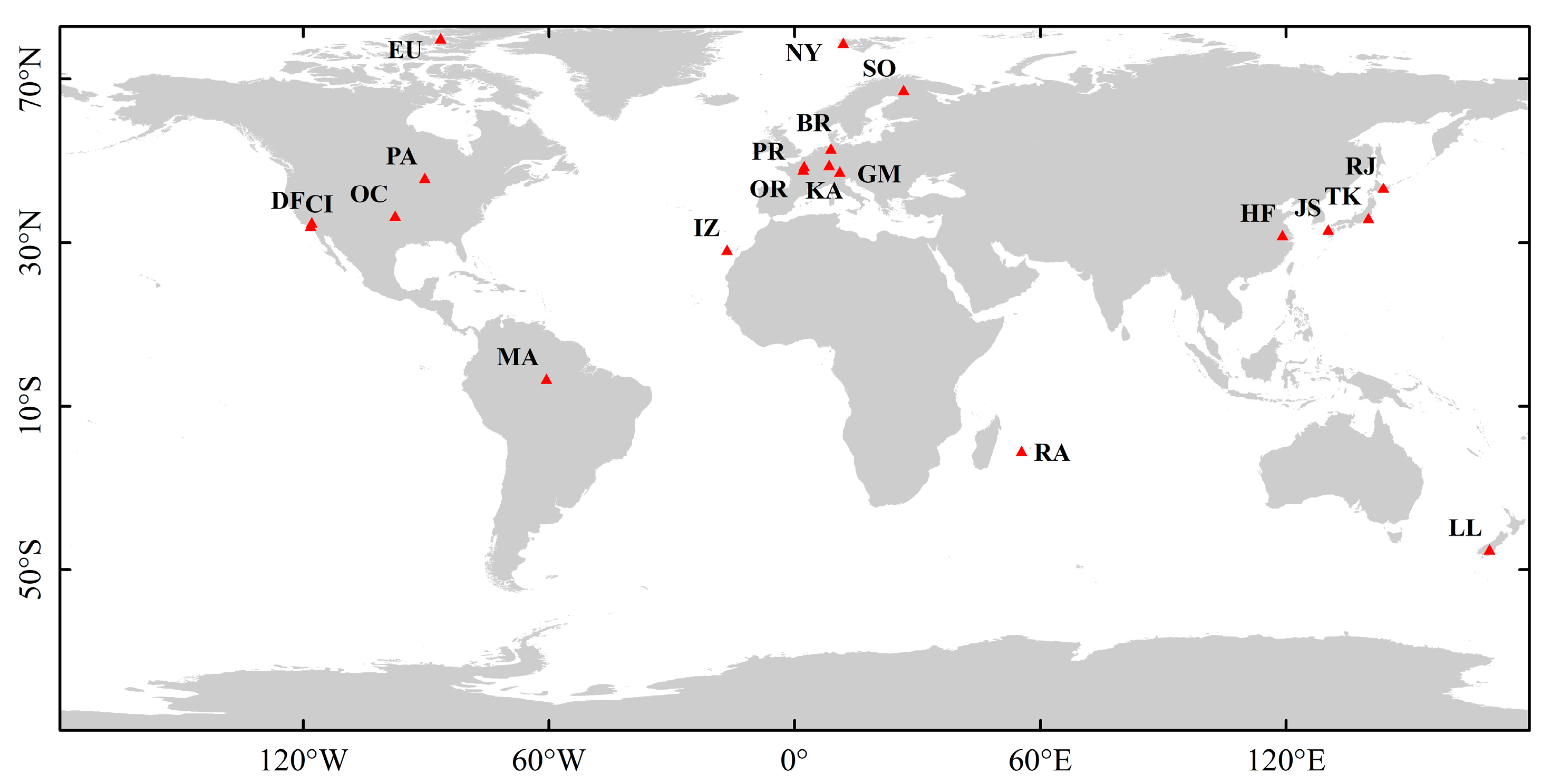

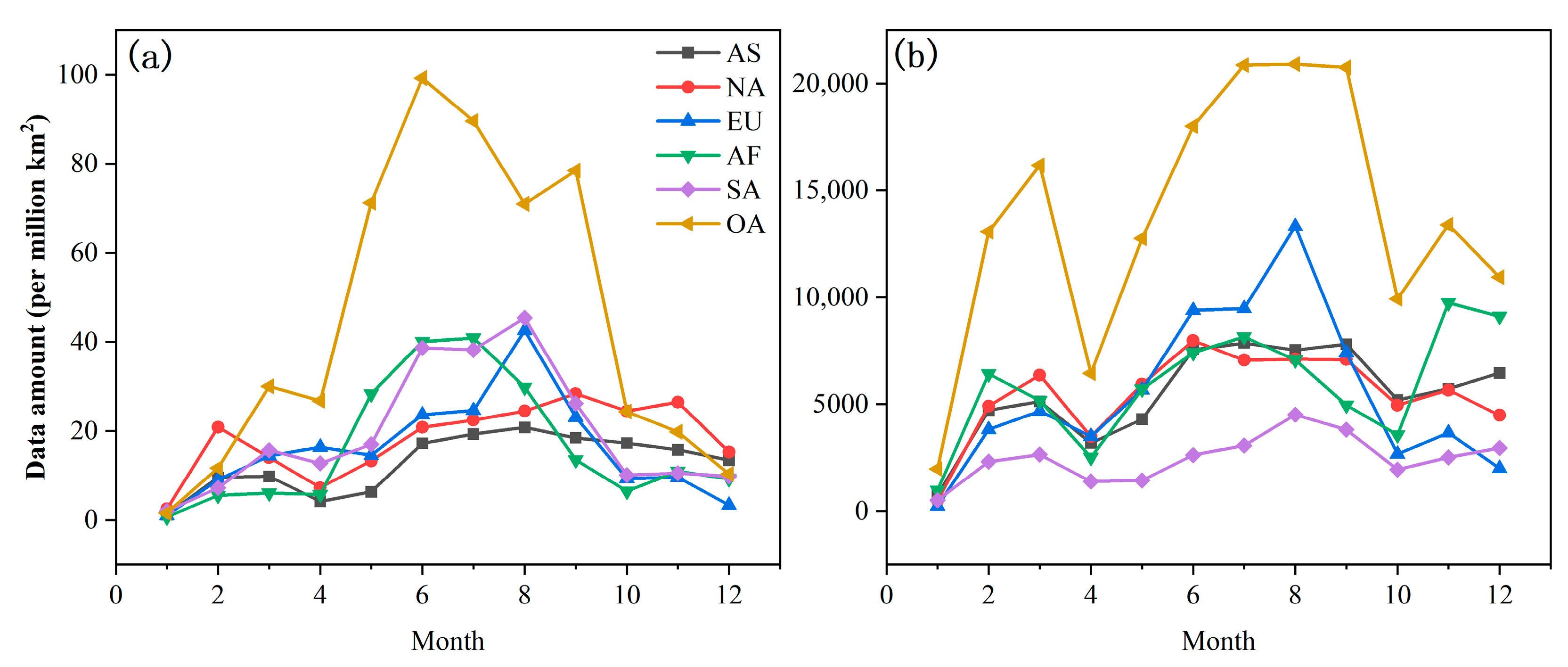

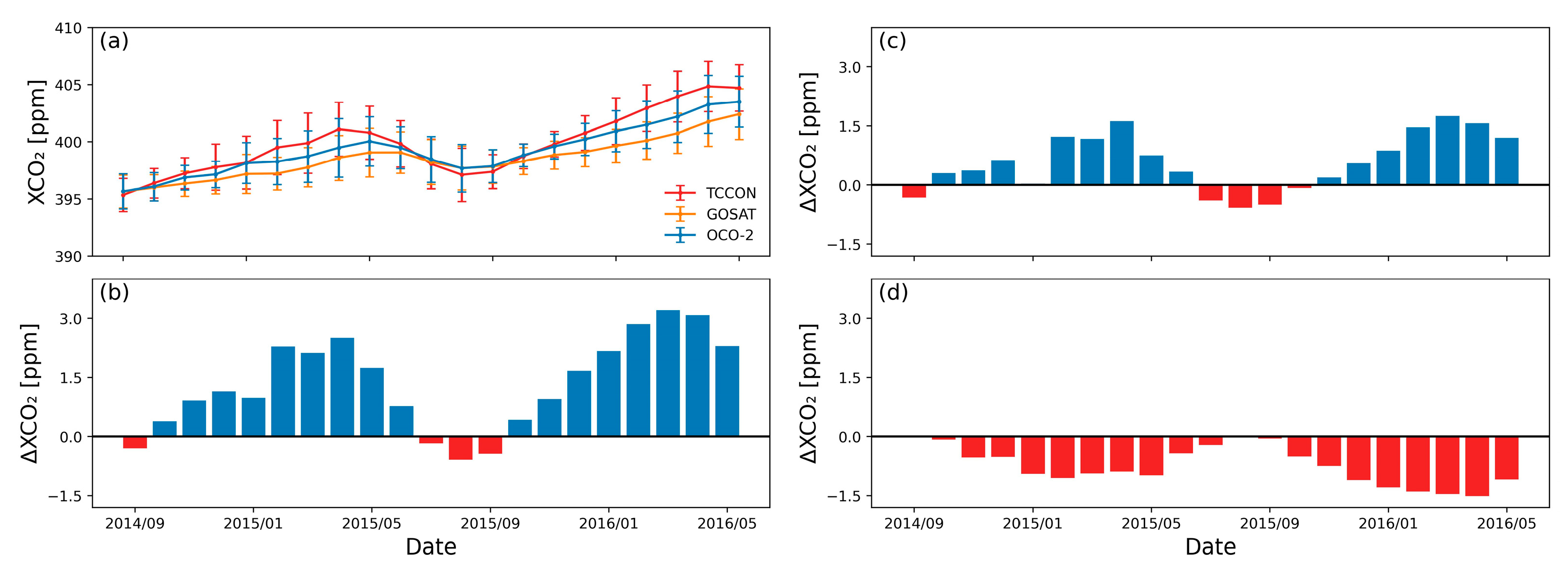
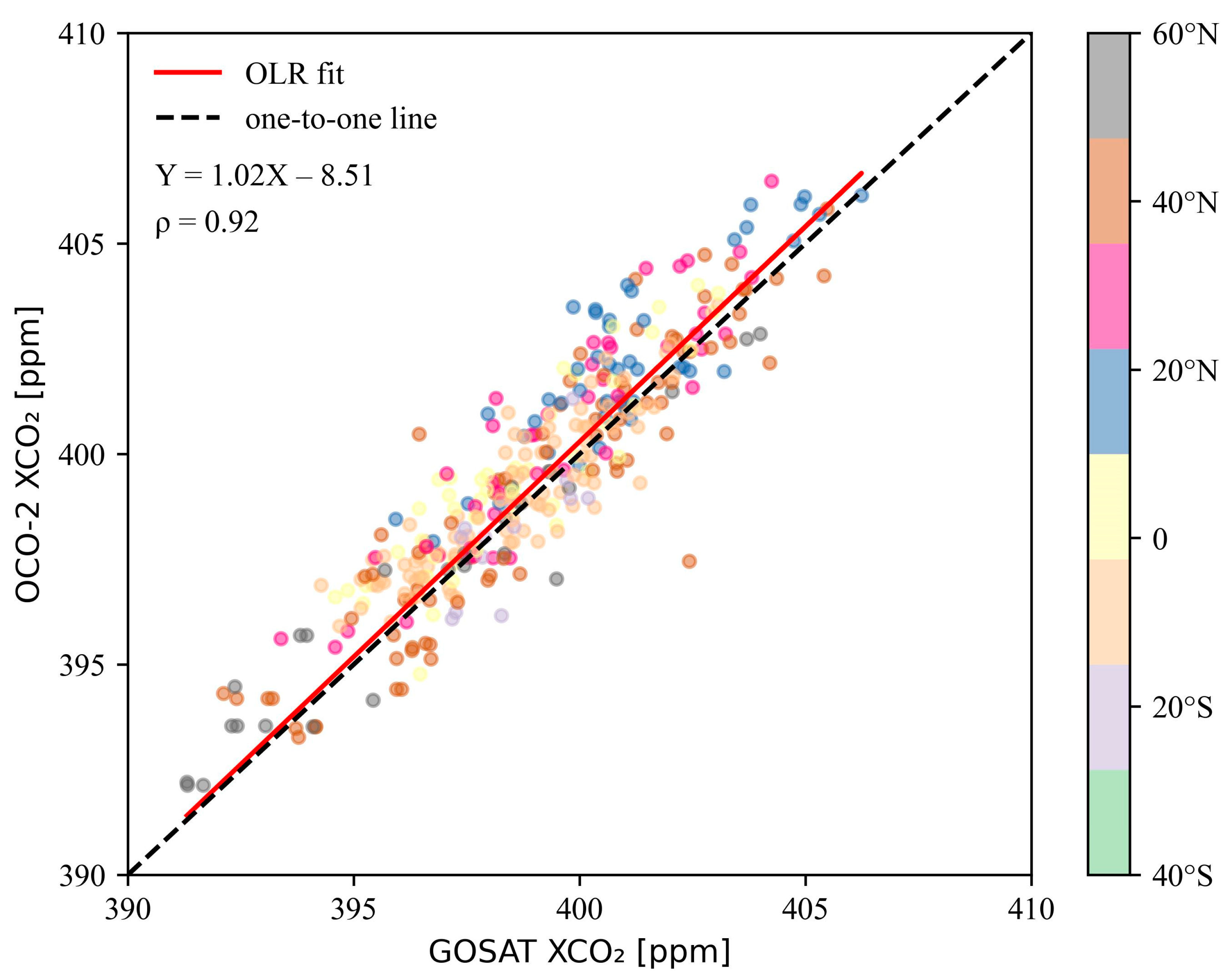
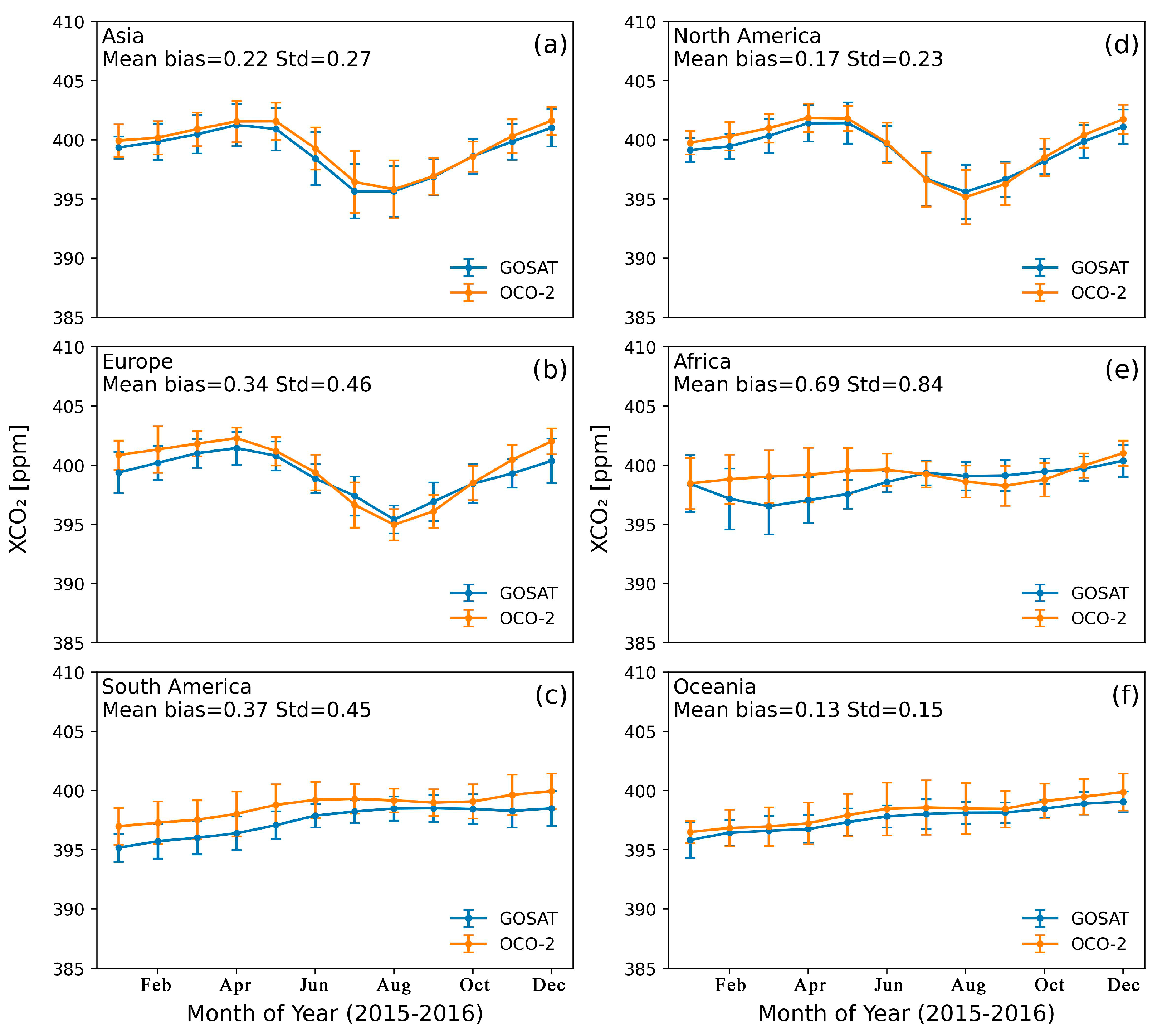

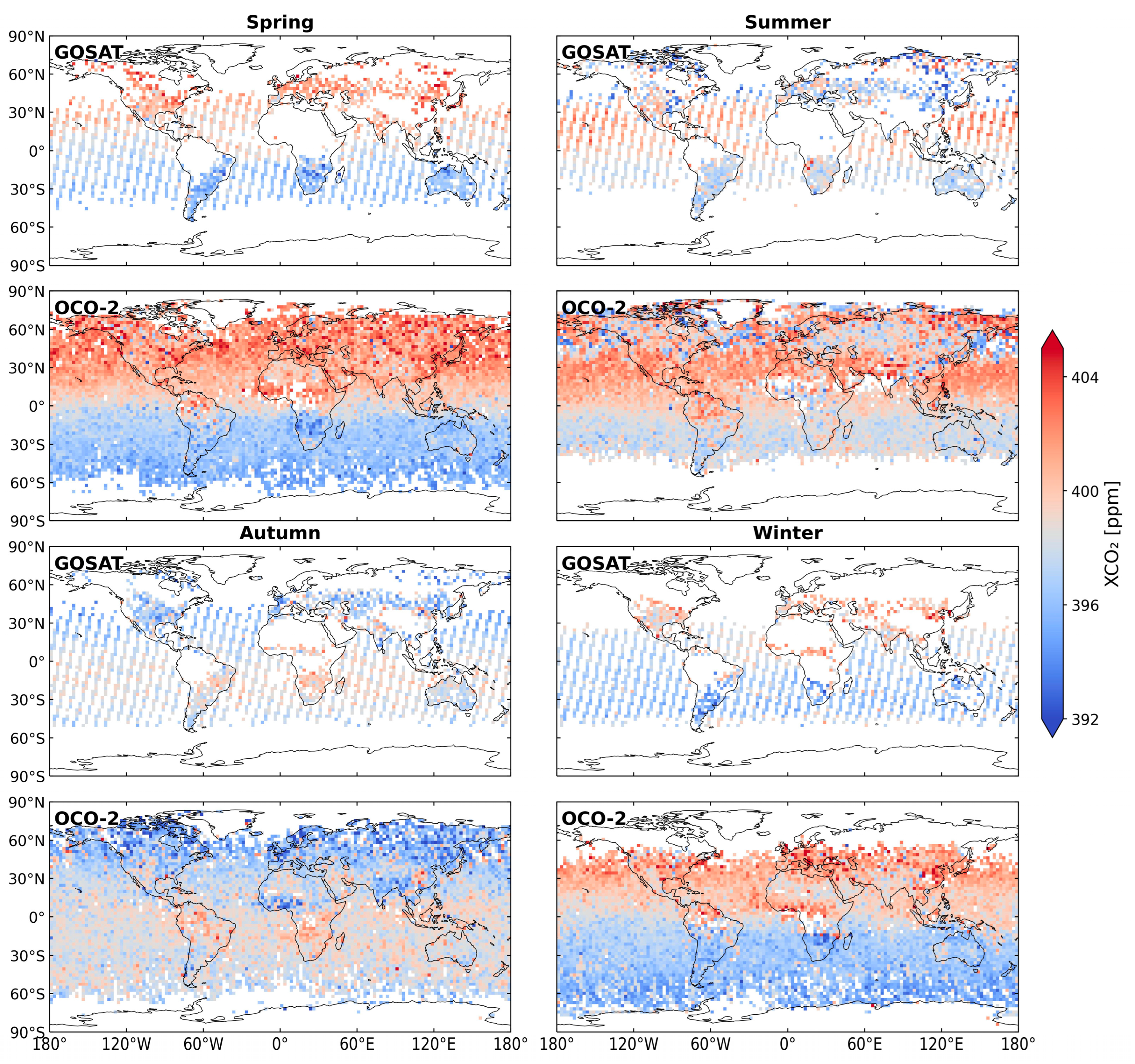
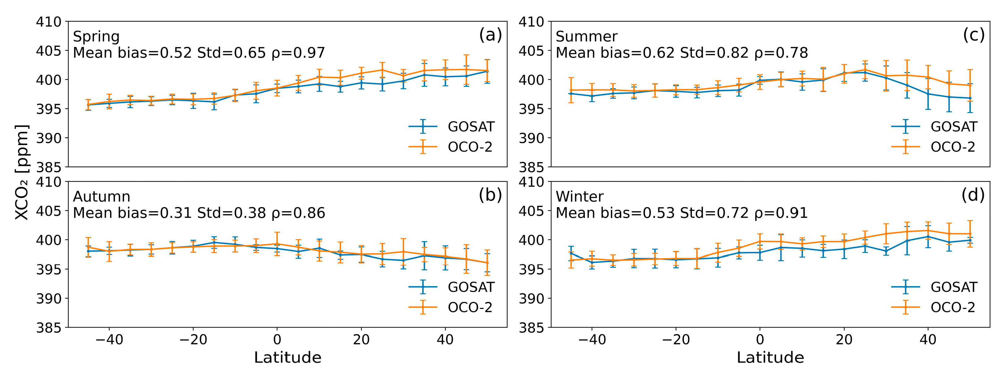
Disclaimer/Publisher’s Note: The statements, opinions and data contained in all publications are solely those of the individual author(s) and contributor(s) and not of MDPI and/or the editor(s). MDPI and/or the editor(s) disclaim responsibility for any injury to people or property resulting from any ideas, methods, instructions or products referred to in the content. |
© 2023 by the authors. Licensee MDPI, Basel, Switzerland. This article is an open access article distributed under the terms and conditions of the Creative Commons Attribution (CC BY) license (https://creativecommons.org/licenses/by/4.0/).