Abstract
The transmitted beam of frequency diversity array (FDA) has the range–angle–time coupling property, which has essential applicative potential in angle deception and active anti-jamming. In this paper, the concept of time index within pulse is introduced. Firstly, the phase characteristics of FDA-transmitted signals based on the time index within pulse concept are studied. Then, the deceptive angle performance of FDA-transmitted signals is discussed. The theoretical analysis and simulation results show that the phase characteristics of the FDA signal are not related to the range, but to the time index within pulse. With the phase center as the reference point, the phase is equal as long as the time index within the pulse is the same. Angle deception and active anti-jamming can be achieved using the optimized frequency increment of each FDA.
1. Introduction
Frequency diversity array (FDA) has attracted wide attention since it was first proposed [1]. Unlike phased array (PA), which transmits signals with the same carrier frequency, FDA introduces different frequency increments in each array element so that the transmitted beam is range–angle–time-dependent [2,3,4]. When the frequency increment is zero, FDA simplifies to PA so that PA is a particular case for FDA. Due to the increased freedom of range dimension and improved capacity for information processing, FDA has potential application value in many areas, such as radar detection, positioning, and anti-jamming [5,6].
When the frequency increment of FDA increases linearly, its transmitted beam is coupled in range, angle, and time [7]. Regarding de-coupling, many scholars pay attention to the transmitted beam with a non-uniform increase in the frequency increment of FDA. For example, Log frequency offset [8], cubic frequency offset [9], multi-carrier frequency [10], random frequency offset [11], time-dependent frequency offset [12,13], and genetic algorithm optimization frequency increment [14] are used to achieve beam focusing. However, these methods ignore the influence of the time factor and lead to an instantaneous beam. The literature [15] points out that these methods ignore the signal propagation process, and that the beam cannot only focus on a specific position in space and last for a particular time. The literature [16] emphasizes that the propagation process of the electromagnetic wave cannot be ignored. The literature [17,18,19] has obtained the corrected pulse FDA expression by analyzing the frequency–phase and time–range relationships. Furthermore, the literature [20] points out that the FDA beam is time–angle-dependent, not range-dependent, and that a reasonable signal processing scheme at the receiving end is necessary for activating FDA distance correlation [21,22]. Ref. [23] further explains the relationship between the time index within pulse and real-time, which is similar to the relationship between radar fast time and slow time. However, ref. [20] does not give the relationship between the time index within pulse and the phase.
Radar needs not only a good detection performance, but also a good capacity for anti-jamming. With the development of digital radio frequency memory (DRFM), active jammers can produce complex and flexible jamming signals, which seriously threaten the performance of radar systems. Therefore, radar anti-jamming technology is essential. FDA radar beam can activate range correlation. Based on this, many scholars have researched the suppression of deceptive interference [24,25,26,27,28,29,30]. However, these methods are targeted at specific interference scenes. The literature [31] discusses the low interception performance of FDA-transmitted signals, indicating that FDA-transmitted signals are less likely to be intercepted by jammers than PA-transmitted signals, thus making it difficult for jammers to target jamming signals in arrays. The literature [32] has preliminarily discussed the possibility of FDA’s resistance to interferometer-based direction of arrival (DOA) reconnaissance. On this basis, the literature [33,34,35,36,37] has studied the phase characteristics of FDA’s transmitted signals and their cheating effect on the interferometer. However, all such studied have taken the spatial phase and range into one-to-one correspondence, have not considered the influence of wave propagation, and have ignored the time index within pulse. At the same time, it has also been ignored that interferometer direction finding is based on its measurement and the estimation of the incident signal frequency, and that it then estimates the direction of the phase center of the received signal. Inspired by the study of uniform linear PA phase centers in the literature [38], based on the time index within pulse, this paper discusses the phase characteristics of FDA-transmitted signals and the calculation method of the phase center, and uses the adjustable phase center to achieve FDA active anti-jamming.
Finally, for the jammer based on the interferometer to determine the position of the array radar, this paper proposes an active anti-jamming method so that the jammer signal cannot be aligned with the array, even by setting multiple phase center flashing so that the jammer completes the direction finding with difficulty. The main contributions of this paper are as follows:
- The phase characteristics of the FDA-transmitted signal based on the time index within pulse are analyzed.
- The phase center of the FDA-transmitted signal is calculated, and the theoretical basis of FDA angle deception is analyzed by adjusting the phase center.
- An active anti-jamming algorithm based on the FDA phase center is proposed by optimizing each element’s frequency increment.
The rest of this paper is arranged as follows. Section 2 and Section 3 derive and analyze the phase characteristics of PA and FDA, respectively. Next, Section 4 presents the calculation method of the phase center of the array-transmitted signal and discusses how FDA implements angle deception. Finally, the theoretical analysis is verified through simulation in Section 5, and the conclusion is given in Section 6.
Notation: We use boldface for vectors and matrices . Scalar a is denoted by italics. The transpose, conjugate and conjugate transpose are denoted by the symbols , and , respectively. The letter j represents the imaginary unit (i.e., ).
2. Phase Characteristics of PA
In this section, we first analyze the propagation characteristics of electromagnetic waves to fully understand the relationship between real-time and the time index within pulse, and determine the real-time–phase relationship. Then, the time–angle–phase relationship of the transmitted signal is determined by analyzing the phase of the PA signal based on the time index within pulse.
2.1. Phase Propagation Analysis
Set the time index within pulse as and the real-time as . The pulse signal with the carrier frequency can be expressed as follows:
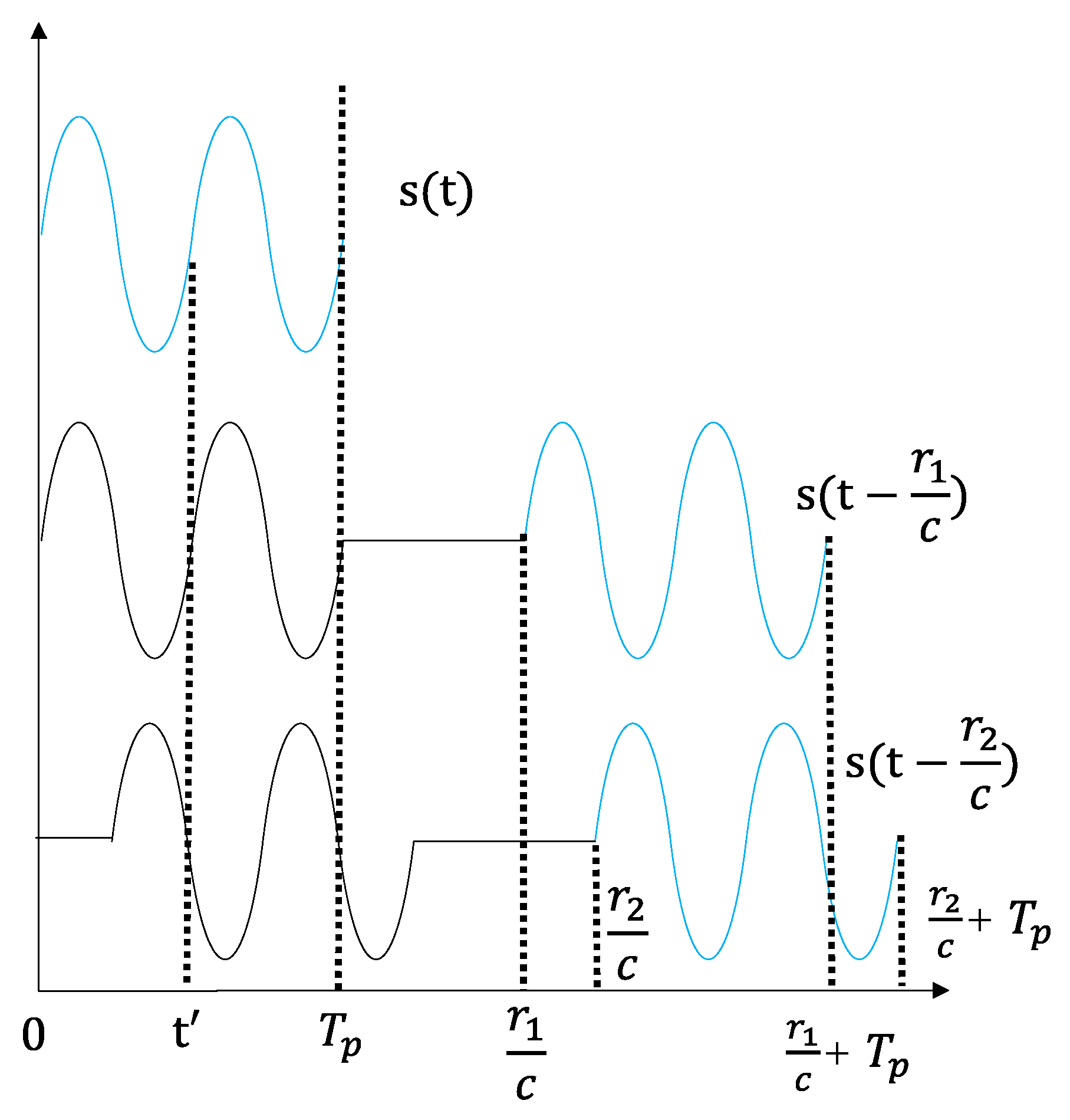
where stands for the pulse duration when the pulse signal propagates to and ; the phase changes in the propagation process are shown in Figure 1.
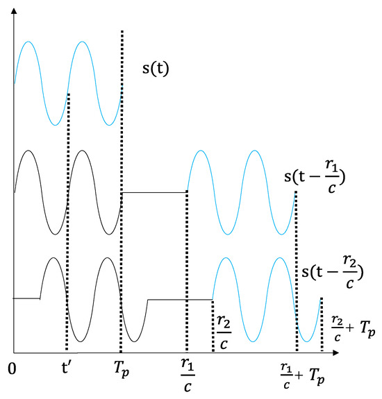
Figure 1.
Phase-change process of pulse signal.
The pulse signals of the two moments can be expressed as follows:
Figure 1 shows that the pulse signal phase is related to its real-time spatial propagation, which can be divided into two parts: propagation delay and the time index within pulse . Further, when the time index within pulse is equal, the phases of the pulse signals are also equal. In order to highlight the vital parameter of the time index within pulse, we let ; then, (3) and (4) can be unified into (5).
Equation (5) can uniformly represent the pulse signals transmitted to different ranges, which means that the phase of the pulse signal is only related to the time index within pulse but has nothing to do with the propagation delay. Therefore, the time index within pulse can be used to replace the real-time when analyzing the phase of the pulse signal.
The continuous wave signal can be regarded as the pulse signal with an infinite pulse time, and its phase is only related to the time index within pulse. In a word, the phase of both the pulse signal and continuous-wave (CW) signal is only related to the time index within pulse and has nothing to do with the propagation delay. The propagation delay is related to the range, which means that the electromagnetic wave signal constantly propagates forward.
2.2. PA Signal Analysis
Through the above analysis, it is clear that the signal phase is related to the time index within pulse. In this section, we will analyze the phase characteristics of PA emission signals so that we can accurately understand the phase characteristics of FDA emission signals.
Consider a uniform linear PA with M isotropic antennas, as shown in Figure 2.
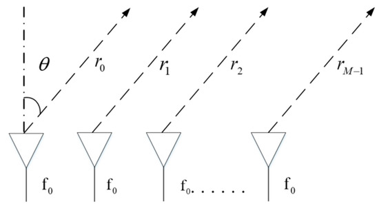
Figure 2.
Uniform linear phased array.
The carrier frequency is and the array spacing is . When it propagates to the far field with range and angle , the signal can be expressed as follows:
where . Under the far-field narrow-band condition, the envelope is approximately invariant, as follows:
Meanwhile, we replace the real-time with the time index within pulse , and Equation (6) can be further expressed as follows:
According to (8), the amplitude and phase of the PA-transmitted signal in the far field can be expressed as follows:
According to (10), the far-field phase of the PA-transmitted signal is related to the time index within pulse, angle, and array spacing, but not to the range; in addition, the phase of each point in the far field changes with the change in the time index within pulse. During the reconnaissance phase, the phase measured by the jammer is as follows:
3. FDA Phase Characteristics
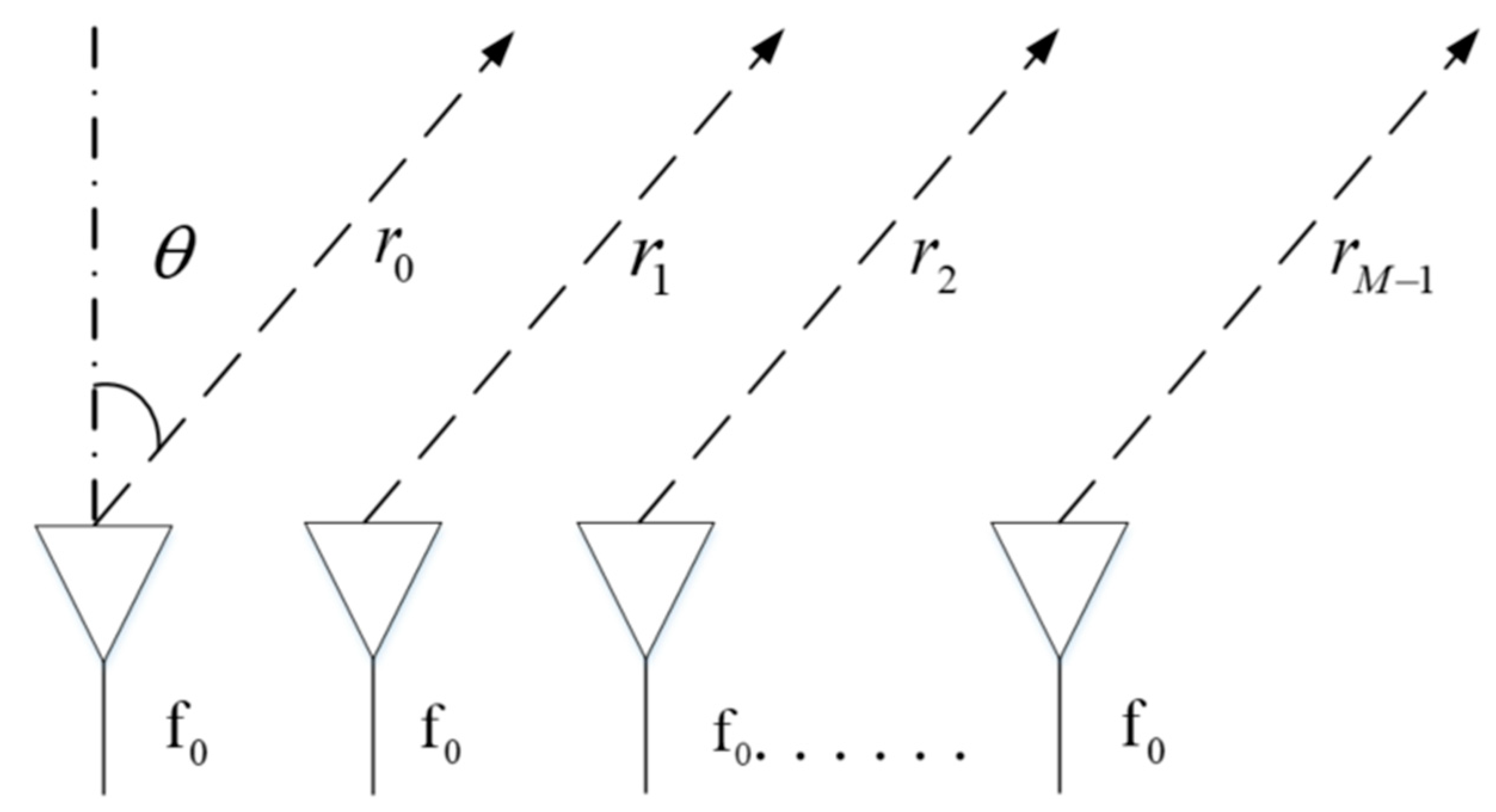
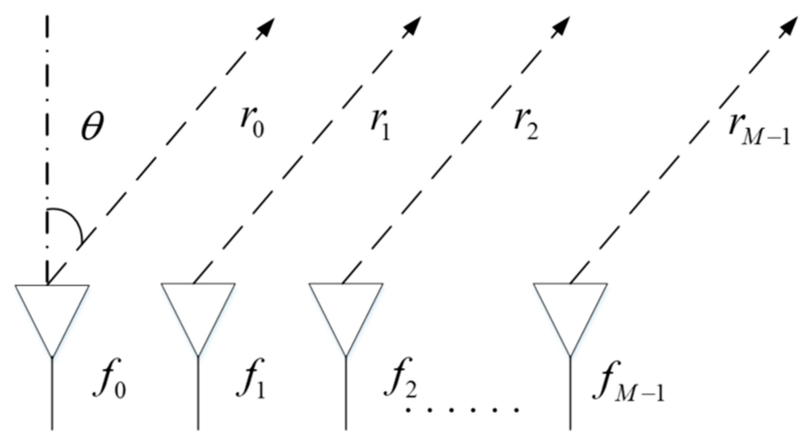
Consider a uniformly linear FDA with M isotropic antennas, as shown in Figure 3.
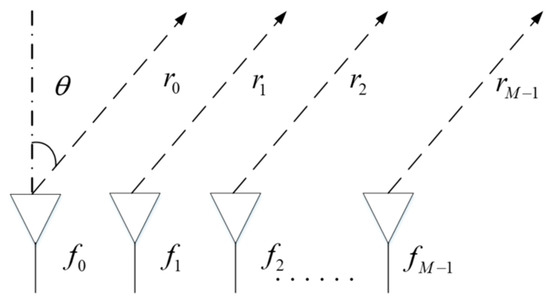
Figure 3.
Uniform linear frequency diversity array.
The carrier frequency of each array is , and the array spacing is . When it propagates to the far field with range and angle , the signal can be expressed as follows:
where . First, consider the FDA with linearly increasing frequency offset (LIFDA), namely . Assuming that the envelope of the far-field condition is approximately unchanged and that the real-time is replaced by the time index within pulse , Equation (12) can be further expressed as follows:
It can be concluded from (13) that the amplitude and phase of the LIFDA in the far field are, respectively, expressed as follows:
According to (15), the far-field phase characteristics of the LIFDA are similar to those of PA, which is related to the time index within pulse, angle, and array spacing, but not to the range. The phase of each point in the far field changes with the change in the time index within pulse. The different phase of PA and FDA in the same far-field location is due to their different carrier frequencies. The PA carrier frequency is , while the equivalent carrier frequency of the LIFDA is , which is the average of each array carrier frequency. During the reconnaissance phase, the phase measured by the jammer is as follows:
Further, consider an FDA with an arbitrary frequency offset (AIFDA), assuming that the frequency offset can be any value. By replacing the real-time with the time index within pulse , (12) can be further expressed as follows:
For observation (18), we found it challenging to adjust to a form similar to . Therefore, we used Matlab function “angle” to extract the phase of (18), which can be expressed as follows:
The phase of the AFFDA in the far field can be obtained using (19). By observing (18) and (19), it can be seen that the far-field phase of the FDA-transmitted signal is related to the time index within pulse, angle, array spacing, and frequency increment, but has nothing to do with the range. The phase changes with the change in the time index within pulse. Furthermore, the phase of the far-field point can be modulated by setting an appropriate frequency increment, which is also the theoretical basis for implementing FDA angle deception and active anti-jamming.
4. Phase Center and Angle Deception
4.1. Phase Center
As shown in Figure 4, a single-baseline phase interferometer was considered to measure the phase of FDA-transmitted signals to obtain the DOA. It is worth noting that the DOA points to the phase center of the array signal.
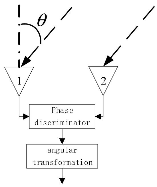
Figure 4.
Principle of single-baseline phase interferometer.
The single-baseline phase interferometer consists of two channels. The line formed by antenna 1 and antenna 2 is called the interferometer baseline. If the array-equivalent phase center is far enough from the receiver, the electromagnetic wave received is approximately a plane wave, and the angle between the incoming wave direction and the antenna is . Then, the time of the plane wave arriving at antenna 1 and antenna 2 is different, and there is a phase difference , which is related to the carrier equivalent frequency . This can be expressed as follows:
If the gains of the two channels are entirely consistent, then the DOA of the array radiation signal can be written as follows after angle transformation:
Phase ambiguity is discussed in ref. [27]. This paper does not consider phase ambiguity, and the DOA points to the phase center of the array. The measurement of phase difference depends on the equivalent frequency of the incident array signal. Therefore, the FDA has the potential to mislead the interferometer’s measurement of the DOA by optimizing the phase difference in the frequency increment modulation of each array element, meaning that ultimately the jammer cannot align the array in space.
The phase center of the array plays a vital role in the direction-finding process of the jammer, so we need to analyze the phase center of the array. According to IEEE standards, the phase center is defined as the position of the point associated with the antenna. If the phase center is used as the reference point, the phase of the radiant sphere surface is constant. We can conclude that if the phase center is taken as the reference point, its phase is only related to the time index within pulse and not to the angle. If the time index within pulse is the same, the phase of the signals is equal regardless of the angle.
Let the range between the phase center and the first antenna be . Firstly, PA is considered. With the phase center as the reference point, the PA-transmitted signal can be expressed as follows:
By replacing the real-time with the time index within pulse , (22) can be expressed as follows:
In this case, the far-field phase characteristics can be expressed as follows:
Because the reference point is the phase center, is required; the phase has nothing to do with the angle. In this case, the coefficient sum of the angle should be zero, so the phase center can be expressed as follows:
Equation (25) indicates that the phase center of the PA-transmitted signal is located in the geometric center of PA, which the phase interferometer can accurately measure. Therefore, PA has no capacity for angle deception according to the phase interferometer.
Then, considering the FDA, with the phase center as the reference point, its transmitted signal can be expressed as follows:
For the FDA, the LIFDA is first analyzed. By replacing the real-time with the time index within pulse , (26) can be expressed as follows:
According to (27), the far-field phase characteristics of the LIFDA-transmitted signals can be expressed as follows:
where . Because the reference point is the phase center, the phase has nothing to do with the angle, that is, . Therefore, the phase center can be expressed as follows:
Through further simplification, (29) can be expressed as follows:
Equation (30) shows that when the frequency increment is zero, the phase center of the FDA-transmitted signal is equal to that of the PA, both located in the geometric center of the array. When , the phase center of the FDA-transmitted signal is related to the ratio of the base carrier frequency and to the center carrier frequency that treats the FDA-transmitted signal as a whole signal. The angle deception of the FDA according to the phase interferometer can be realized by taking the appropriate value of .
Finally, the phase center of the AIFDA-transmitted signal is analyzed. By replacing the real-time with the time index within pulse , (26) can be expressed as follows:
By observing (31), it can be found that it is not easy to extract the phase expression due to the arbitrariness of frequency increment, but it can be found that the phase is related to , , , and . The phase of (31) is extracted by using the function “angle”, which can be expressed as follows:
According to the definition of phase center, the phase of the array signal in space has nothing to do with the angle. When the time index within pulse and frequency increment are determined, the phase at each angle is equal; this can be expressed as following:
Equation (33) shows that after , and are determined, can be calculated.
4.2. Angle Deception
Before analyzing the angle deception, we first discuss obtaining through the use of (33). Then, on this basis, we set the phase center of the virtual radiation source as . Finally, by optimizing the frequency increment , the phase center is located at . At this time, the direction measured using the phase interferometer points to the center of the virtual radiation source, and the FDA angle deception and active anti-interference are realized.
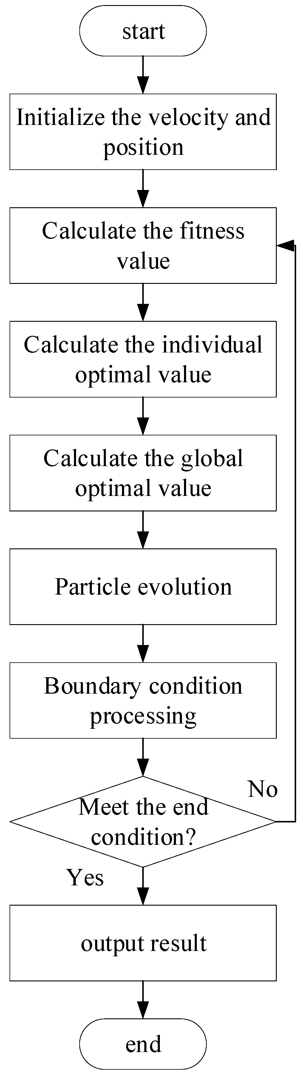
As the parameters in (33) are coupled with each other, it is difficult to derive the phase center directly, so the particle swarm optimization (PSO) algorithm is adopted in this paper. PSO is derived from the well-developed laws of bird population activities, and it uses swarm intelligence to establish a simplified model, comparing the search space of solving problems to the flight space of birds. Each particle represents a possible solution and then solves complex optimization problems through the evolution of population particles. Its operation flow chart is shown in Figure 5.

Figure 5.
Particle swarm optimization flow.
The parameters of PSO include the particle position, particle velocity, individual optimal position, and optimal global position. Suppose that each particle has a dimension and particles form a population, then the position of the -th particle can be expressed as follows:
The velocity of the -th particle is expressed as follows:
The optimal position searched by the -th particle so far is the extreme individual value, which can be expressed as follows:
The optimal position searched by the whole population so far is the extreme global value, expressed as follows:
The process of particle evolution can be expressed as follows:
where and are learning factors. and are uniform random numbers in the range of . stands for the globally optimal particle. is the inertial weight related to the capacity for global convergence, and weighs the capacity for global search and local search. The dynamic inertial weight is used in this paper, and is expressed as follows:
where and represent the maximum and minimum inertial weights, respectively. and represent the current and maximum iterations, respectively.
The optimization problem used to obtain can be expressed as follows:
where and represent the minimum and maximum search values, respectively. is a minimal value, which means that the phases at different angles are approximately equal.
Because is a one-dimensional variable, this paper adopts the discrete PSO algorithm proposed in the literature [39] to solve it. At this time, the value of the particle state space can only be 0 or 1, and the D-dimensional binary particle corresponds to the value of , one by one. The velocity update formula is still (36), and the position update formula is as follows:
where is a random number in . Finally, the expression of the fitness function is determined as (44), according to (41):
When the frequency increment is determined, the phase center can be obtained. Similarly, can be optimized to make the direction finding of the phase interferometer point to the phase center of the virtual radiation source . The optimization problem for obtaining can be expressed as follows:
where and represent the minimum and maximum frequency offset search, respectively. Because is a multidimensional variable, the PSO algorithm proposed in the literature [40] can be adopted. According to (45), the fitness function can be expressed as follows:
Finally, when the frequency increment of the FDA is , it can realize angle deception and active anti-jamming.
5. Simulation Results
The numerical simulation results will be presented in this section. Unless otherwise stated, base carrier frequency , the total number of transmitting array elements is , and the interval is half wavelength . The pulse duration , and the pulse repetition interval .
5.1. PA Phase Characteristics
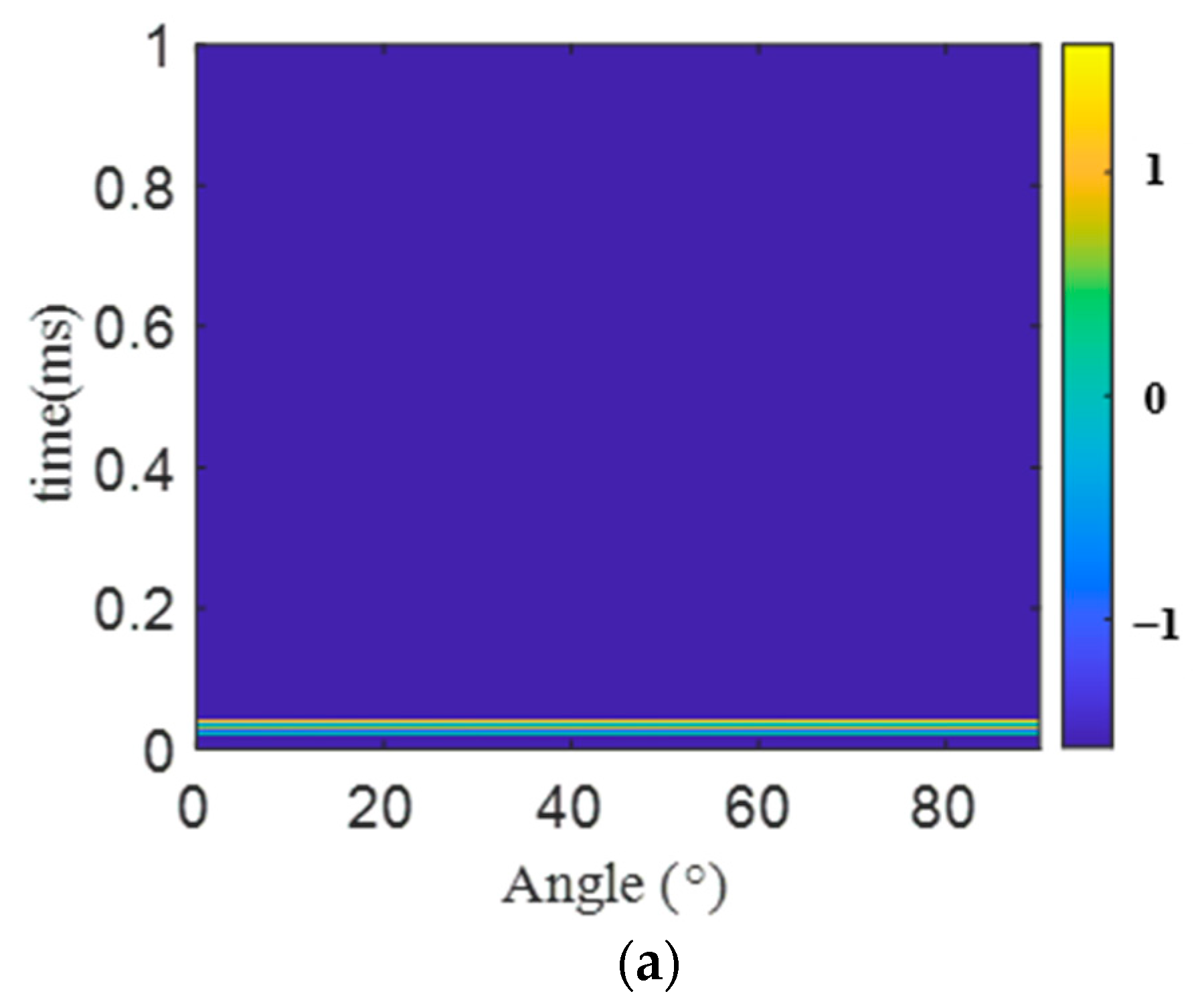
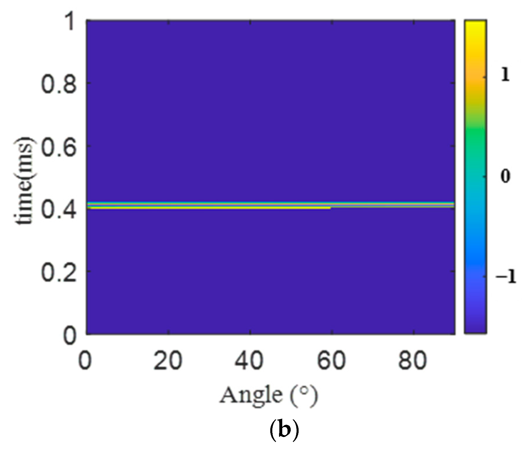
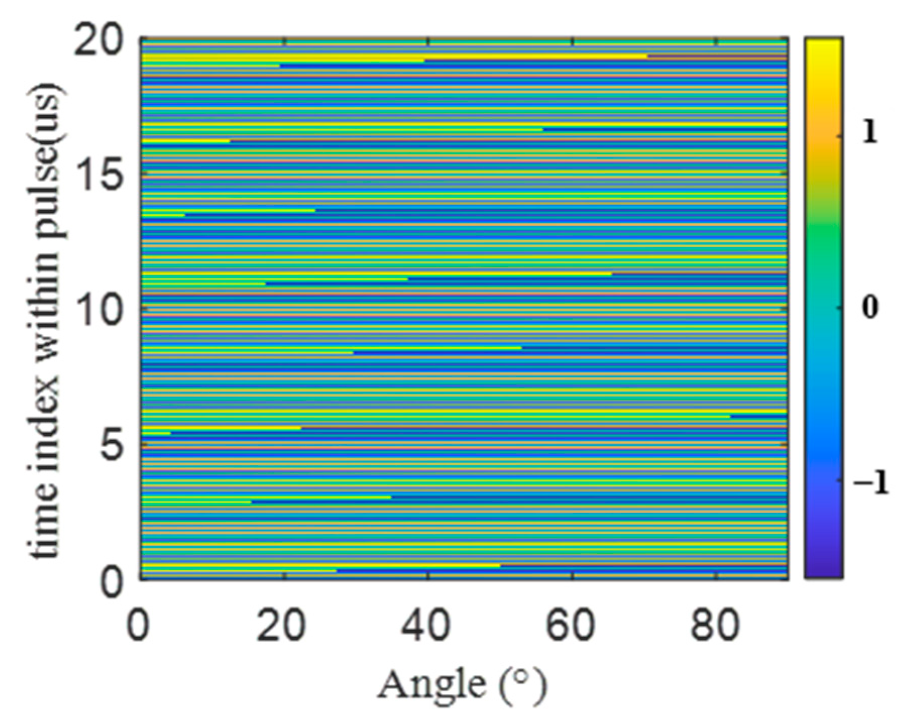
In order to understand the propagation law of the signal phase in space, we simulate the time–angle–phase diagram. When the signal propagates to 6 km, the propagation delay is . In this case, the real-time can be expressed as the propagation delay plus the time index within pulse , and the real-time can be expressed as the propagation delay plus the time index within pulse . When the signal propagates to 120 km, the propagation delay is . In this case, the real-time can be expressed as the propagation delay plus the time index within pulse , and the real-time can be expressed as the propagation delay plus the time index within pulse . The simulation results of the two cases are shown in Figure 6.
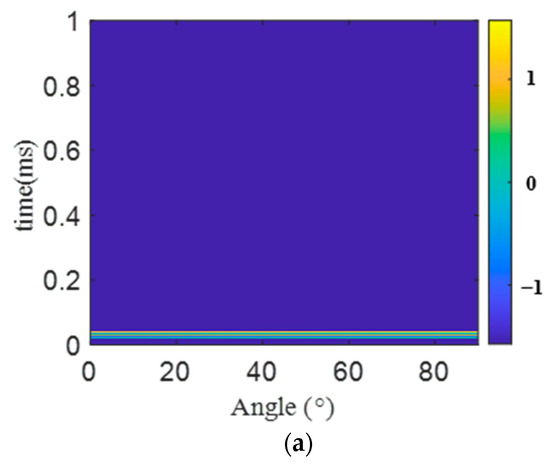

Figure 6.
Time–angle–phase relationship of PA-transmitted signal: (a) ; (b) .
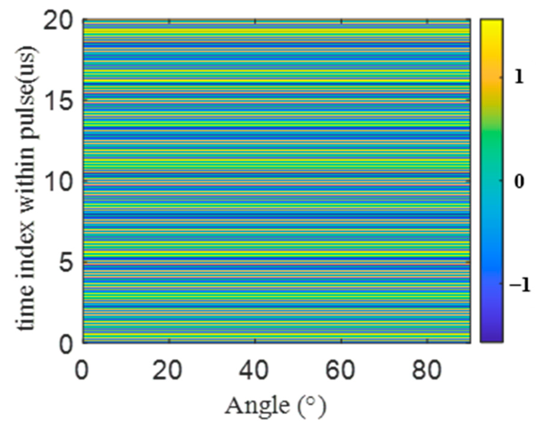
As seen from Figure 6, the phase of the PA-transmitted signal propagates to the far end along with the electromagnetic wave, and each point in space traverses the phase value, independent of the propagation range. In order to understand this problem more clearly, the simulation results of the time index within pulse–angle–phase diagram are given, as shown in Figure 7.
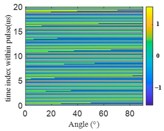
Figure 7.
Time index within pulse–angle–phase relationship of the PA-transmitted signal.
It can be seen from Figure 7 that the value of the phase is related to the angle and the time index within pulse, but not to the range. The phase value of each point in space changes with the time index within pulse. The direction finding of the phase interferometer points to the phase center of the array. According to (23), the phase center of the PA-transmitted signal is . The time index within the pulse–angle–phase diagram of the PA-transmitted signal with as the reference point is shown in Figure 8.
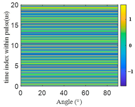
Figure 8.
Time index within pulse–angle–phase relationship of the PA-transmitted signal with the phase center as the reference point.
As shown in Figure 8, with the phase center as the reference point, the phase value in space has nothing to do with the angle and is only related to the time index within pulse. For the interferometer, the baseline is constant, so the time difference within the pulse of the receiving antenna is constant and the phase difference is a constant value, which ultimately enables the phase interferometer to measure the phase center of the PA signal accurately.
5.2. FDA Phase Characteristics
Considering the LIFDA, its frequency increment is set as shown in (47):
where . After the parameters are determined, similar to the previous section, considering the signal propagation to 6 km and 120 km, the simulation results of the time–angle–phase relationship are shown in Figure 9.
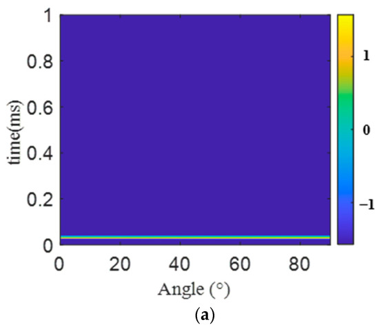
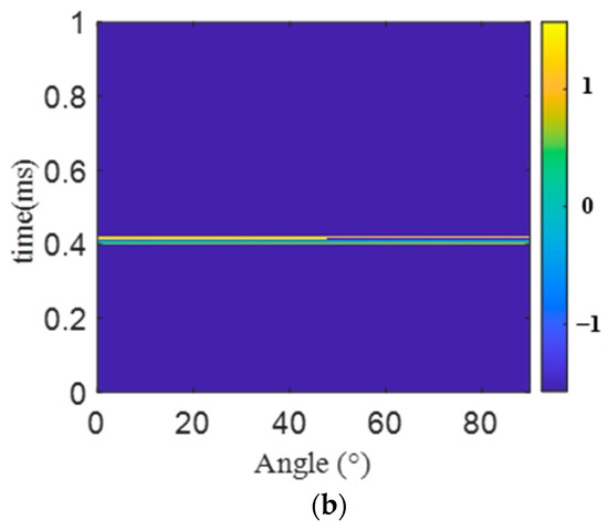
Figure 9.
Time–angle–phase relationship of the LIFDA-transmitted signal: (a) ; (b) .
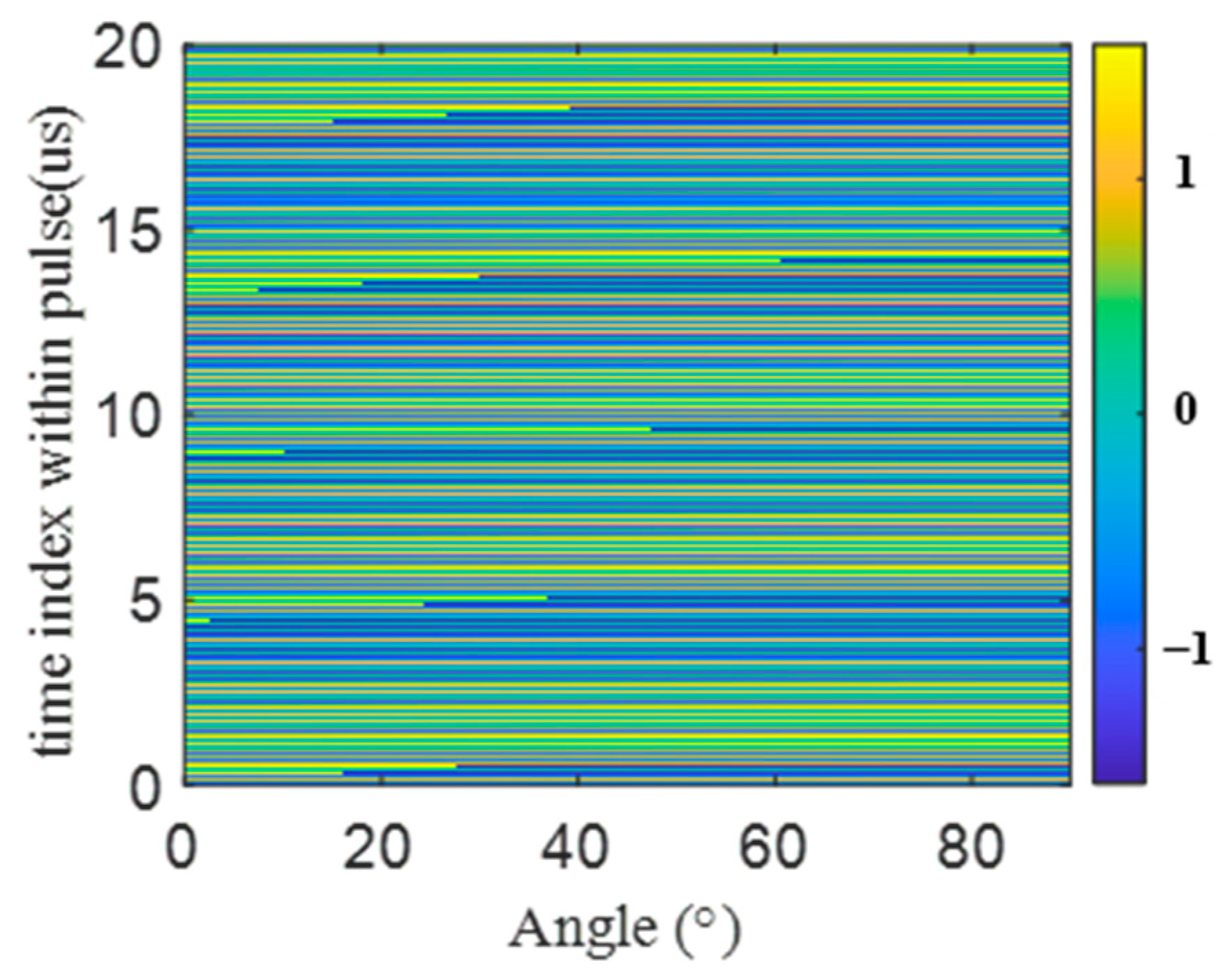
As seen in Figure 9, the phase of the LIFDA-transmitted signal is the same as that of the PA-transmitted signal, which propagates to the far end along with the electromagnetic wave, and each point in space traverses the phase value, which is independent of the propagation range. In order to have a clearer understanding, the simulation results of the time index within the pulse–angle–phase diagram are given, as shown in Figure 10.
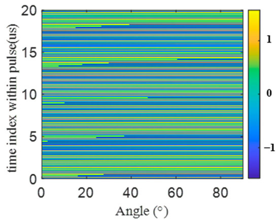
Figure 10.
Time index within the pulse–angle–phase relationship of the LIFDA-transmitted signal.
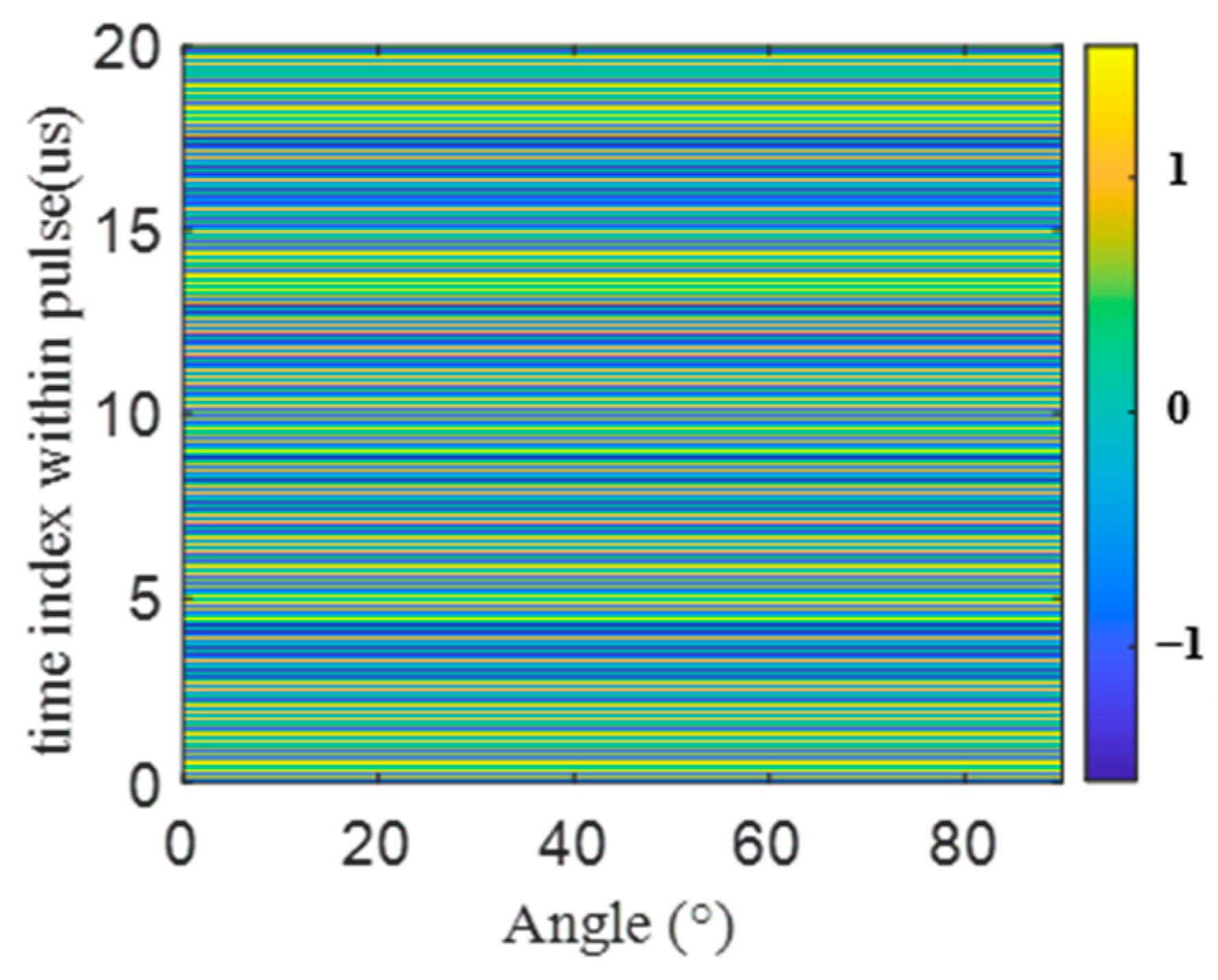
It can be seen from Figure 10 that when the first element is taken as the reference point, the value of the phase is related to the angle and the time index within pulse, but not to the range, and that the phase value of each point in the space changes with the change in the time index within pulse. This paper pays attention to the location of the phase center. According to (28), the phase center of the LIFDA is . The time index within the pulse–angle–phase diagram of the LIFDA-transmitted signal with as the reference point is shown in Figure 11.

Figure 11.
Time index within pulse–angle–phase relationship of the LIFDA-transmitted signal with the phase center as the reference point.
As shown in Figure 11, with the phase center as the reference point, the phase value in space is only related to the time index within the pulse, which is consistent with the theoretical analysis above. At this time, the phase interferometer direction finding is no longer pointed at the center of the array geometry, but slightly offset.
5.3. FDA Angle Deceptive
This section first calculates the phase center of the LIFDA-transmitted signal through the discrete PSO algorithm and verifies the correctness of the algorithm by comparing it with the theoretical analysis above. Then, the phase center of the virtual radiation source is set, and the PSO algorithm obtains the frequency offset of the FDA angle deception. The simulation parameters are set as follows: , , , , , , , , and .
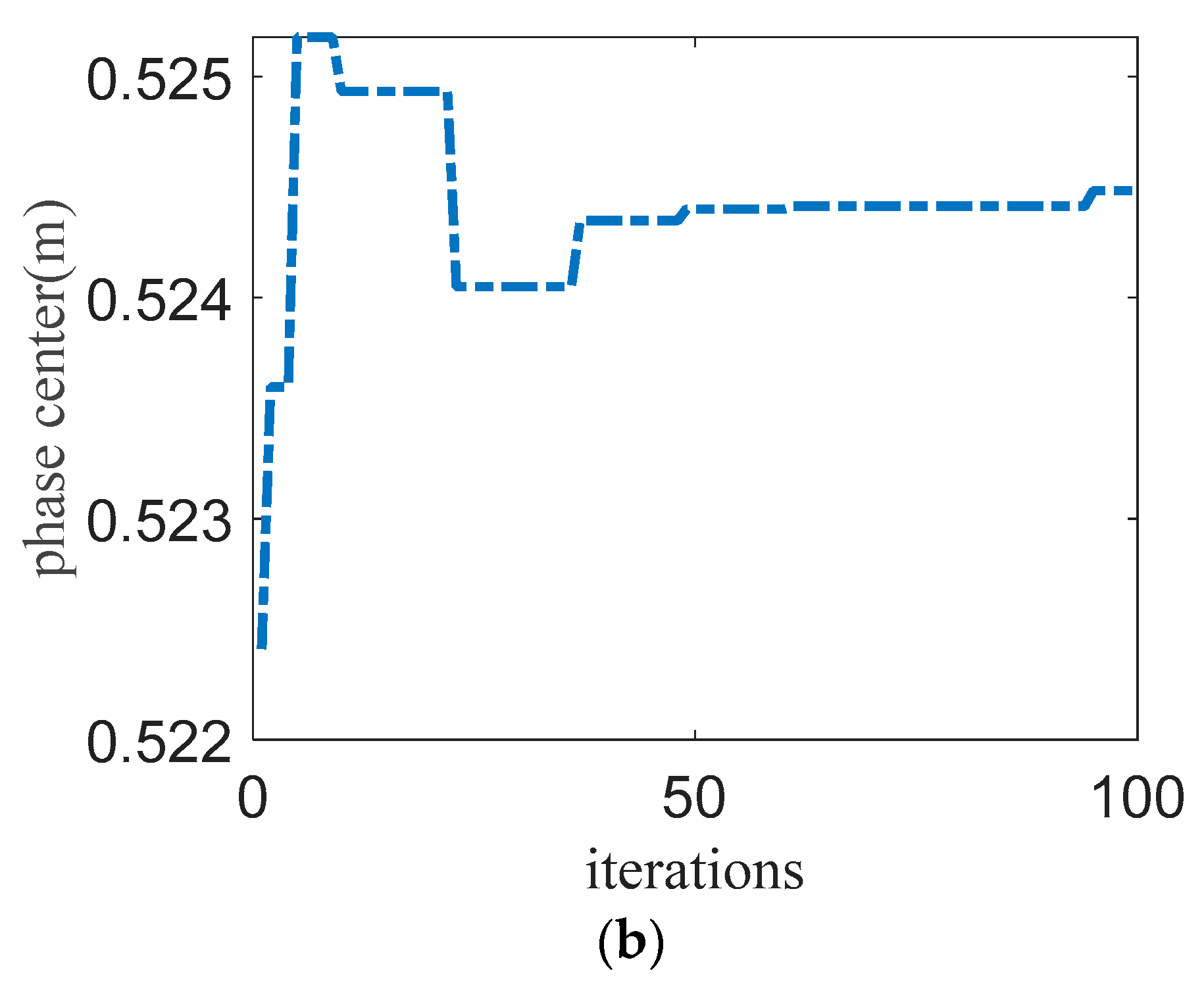
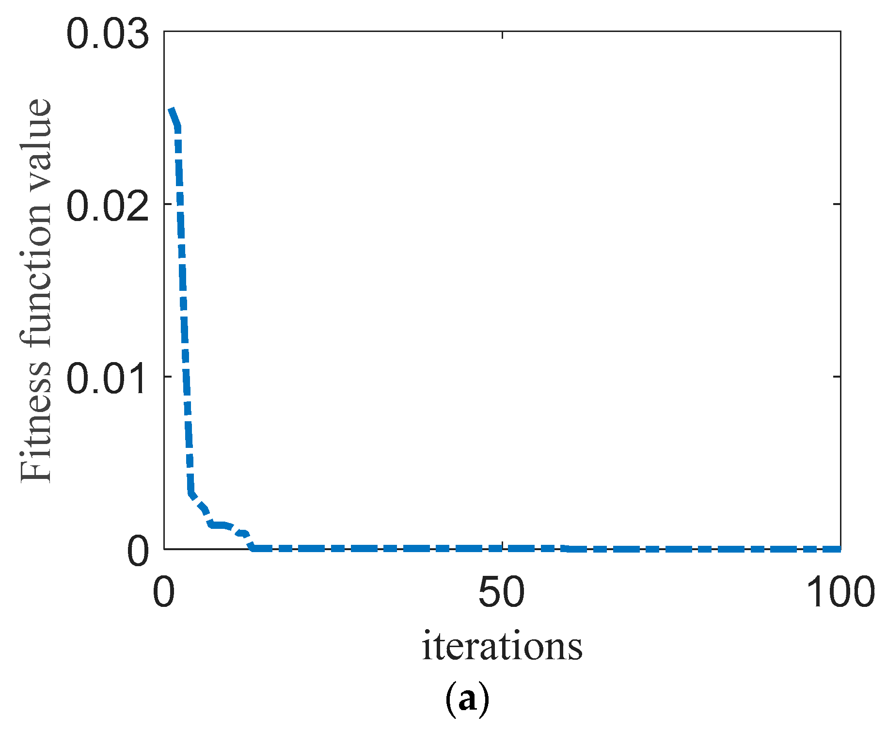
The frequency increment is ; according to (28), phase center . Therefore, the search space is set to , . The fitness function is (42). The simulation results are shown in Figure 12.
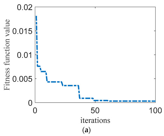
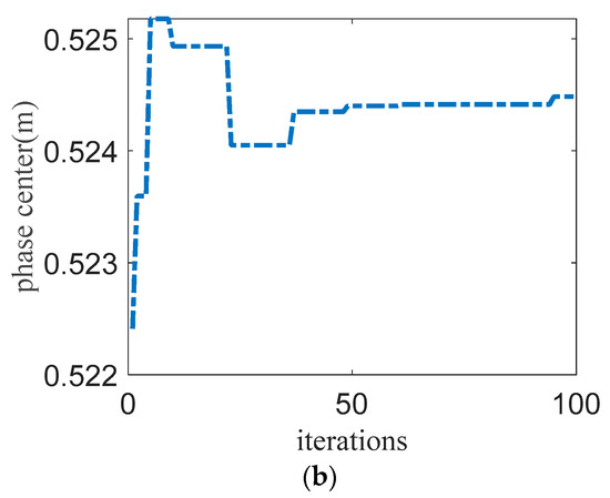
Figure 12.
Relation between the LIFDA optimization results and iteration times: (a) fitness function value; (b) phase center.
It can be seen from Figure 12 that with the increase in the number of iterations, the fitness function approaches 0, indicating that the angles are different, the phases of each point with the same time index within pulse are equal, and the final phase center converges to 0.5244 m, which is consistent with the theory mentioned above.
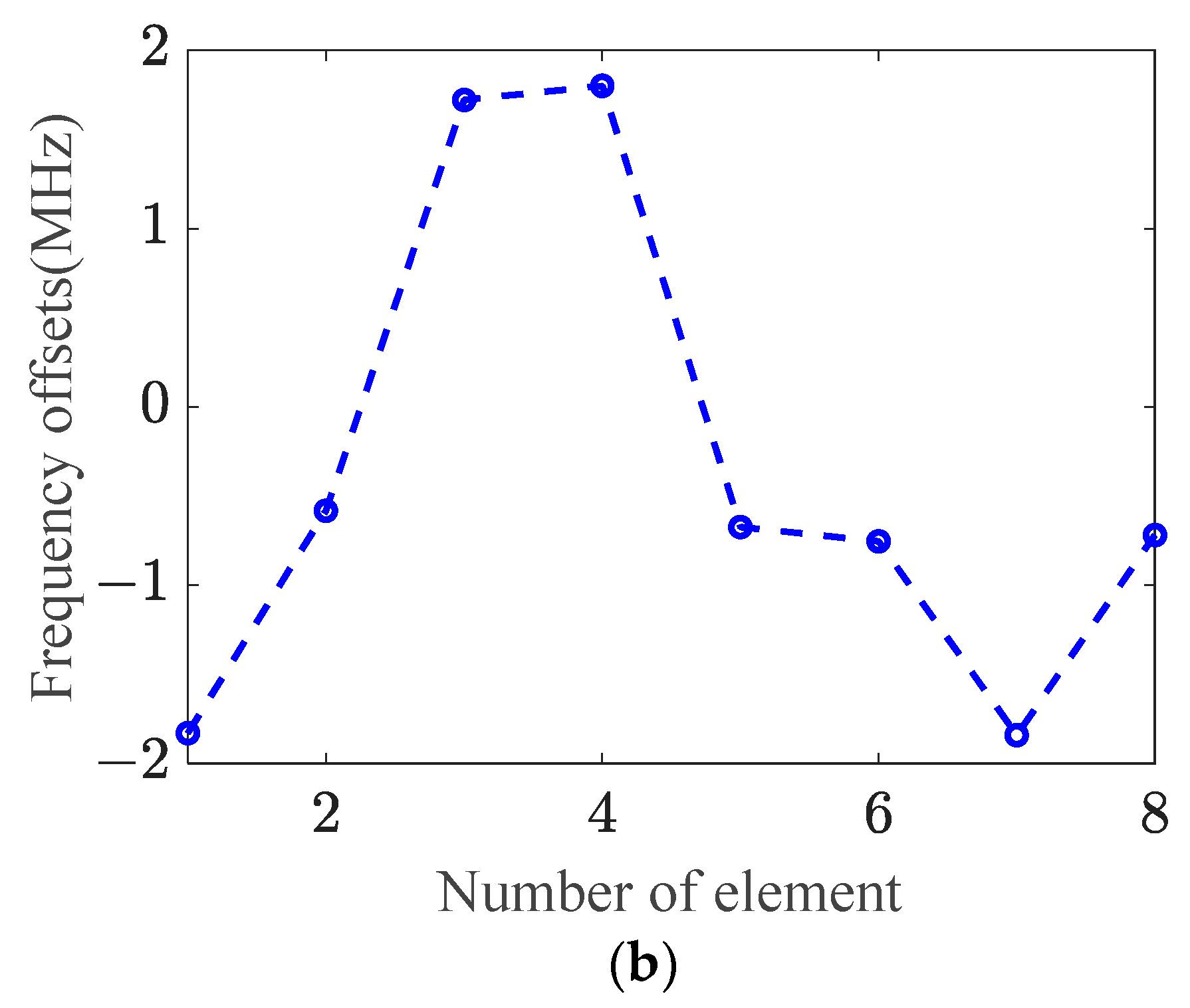
The main lobe of the jammer is large. In order to prevent the array from being affected by the interference signals of the jammer’s main lobe, the phase center of the virtual radiation source should be set as far away from the array as possible. The simulation parameters were set as follows: , , and . The fitness function is (44), and the simulation results are shown in Figure 13. The frequency offsets of each element are shown in Table 1.
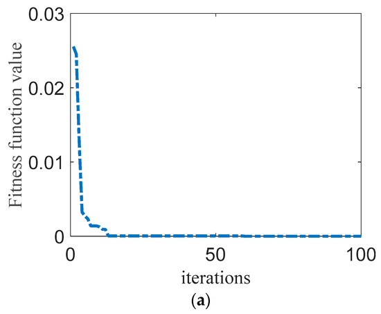
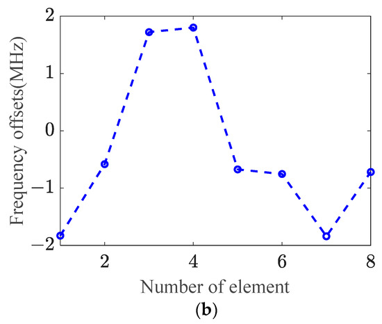
Figure 13.
FDA frequency increment optimization results: (a) fitness function value; (b) frequency increment of each element.

Table 1.
The frequency offsets of each element.
As can be seen from Figure 13, as the number of iterations increases, the fitness function approaches 0, and each array of the FDA adopts the frequency increment, as shown in Figure 12b, to make the phase center far away from the transmitting array, thus realizing the active angle deception of the phase interferometer.
6. Conclusions
This paper studied the phase characteristics of FDA-transmitted signals based on the time index within pulse. In order to fully understand the phase characteristics of the array, the relationship between the time index within pulse and the phase was first analyzed, and the time index within pulse was further understood by discussing the phase characteristics and the phase center of the PA. Secondly, the phase characteristics and phase centers of the FDA-transmitted signals with linearly increasing frequency offset and arbitrary frequency offset were analyzed, and it was concluded that the phase of FDA-transmitted signals is independent of range but related to the time index within pulse, and that its phase center can deviate from the array. The potential of the FDA to cheat the phase interferometer was theoretically elaborated. Furthermore, the PSO algorithm obtained the phase center of the LIFDA, and the algorithm’s effectiveness was verified. Finally, based on this algorithm, the phase center of the virtual radiation source was set, and the frequency increment of the FDA was obtained. The theoretical analysis and simulation experiments have proved that the FDA can realize angle deception and achieve active anti-interference.
Author Contributions
Conceptualization, C.Z. and C.W.; methodology, C.Z. and M.T.; software, C.Z. and M.L.; validation, C.Z., J.G. and L.B.; formal analysis, C.Z.; resources, J.G. and L.B.; writing—original draft preparation, C.Z.; writing—review and editing, C.Z., M.L., M.T. and L.B.; supervision, C.W. and J.G. All authors have read and agreed to the published version of the manuscript.
Funding
This research was funded by the Natural Science Foundation of Shanxi Province under grants 2021JM-222 and National Natural Science Funds of China under grant 62201580.
Data Availability Statement
The data and code used in this study are available upon request to the corresponding author.
Conflicts of Interest
The authors declare no conflict of interest.
References
- Antonik, P.; Wicks, M.C.; Griffiths, H.D.; Baker, C.J. Range-dependent beamforming using element level waveform diversity. In Proceedings of the International Waveform Diversity Design Conference, Lihue, HI, USA, 22–27 January 2006; pp. 1–6. [Google Scholar]
- Huang, J.; Tong, K.F.; Baker, C. Frequency diverse array: Simulation and design. In Proceedings of the 2009 IEEE Radar Conference, Pasadena, CA, USA, 4–8 May 2009. [Google Scholar]
- Huang, J.; Tong, K.F.; Baker, C.J. Frequency diverse array with beam scanning feature. In Proceedings of the Antennas & Propagation Society International Symposium, San Diego, CA, USA, 5–11 July 2008. [Google Scholar]
- Lan, L.; Marino, A.; Aubry, A.; De Maio, A.; Liao, G.; Xu, J.; Zhang, Y. GLRT-based Adaptive Target Detection in FDA-MIMO Radar. IEEE Trans. Aerosp. Electron. Syst. 2021, 57, 597–613. [Google Scholar] [CrossRef]
- Wang, W.-Q. Overview of frequency diverse array in radar and navigation applications. IET Radar Sonar Navig. 2016, 10, 1001–1012. [Google Scholar] [CrossRef]
- Lan, L.; Rosamilia, M.; Aubry, A.; De Maio, A.; Liao, G.; Xu, J. Adaptive Target Detection with Polarimetric FDA-MIMO Radar. IEEE Trans. Aerosp. Electron. Syst. 2023, 59, 2204–2220. [Google Scholar] [CrossRef]
- Secmen, M.; Demir, S.; Hizal, A.; Eker, T. Frequency diverse array antenna with periodic time modulated pattern in range and angle. In Proceedings of the 2007 IEEE Radar Conference, Boston, MA, USA, 17–20 April 2007; pp. 427–430. [Google Scholar]
- Khan, W.; Qureshi, I.M.; Basit, A.; Malik, A.N.; Umar, A. Performance analysis of MIMO-frequency diverse array radar with variable logarithmic offsets. Prog. Electromagn. Res. C 2016, 62, 23–34. [Google Scholar] [CrossRef]
- Gao, K.; Wang, W.Q.; Cai, J.; Xiong, J. Decoupled frequency diverse array range-angle-dependent beampattern synthesis using non-linearly increasing frequency offsets. IET Microw. Antennas Propag. 2016, 10, 880–884. [Google Scholar] [CrossRef]
- Shao, H.; Dai, J.; Xiong, J.; Chen, H.; Wang, W.-Q. Dot-shaped range-angle beampattern synthesis for frequency diverse array. IEEE Antennas Wirel. Propag. Lett. 2016, 15, 1703–1706. [Google Scholar] [CrossRef]
- Liu, Y.; Ruan, H.; Wang, L.; Nehorai, A. The random frequency diverse array: A new antenna structure for uncoupled direction-range indication in active sensing. IEEE J. Sel. Top. Signal Process. 2017, 11, 295–308. [Google Scholar] [CrossRef]
- Khan, W.; Qureshi, I.M. Frequency diverse array radar with time-dependent frequency offset. IEEE Antennas Wirel. Propag. Lett. 2014, 13, 758–761. [Google Scholar] [CrossRef]
- Han, S.; Fan, C.; Huang, X. Frequency diverse array with time-dependent transmit weights. In Proceedings of the IEEE 13th International Conference on Signal Processing, Chengdu, China, 6–10 November 2016; pp. 448–451. [Google Scholar]
- Xiong, J.; Wang, W.-Q.; Shao, H.; Chen, H. Frequency diverse array transmit beampattern optimization with genetic algorithm. IEEE Antennas Wirel. Propag. Lett. 2017, 16, 469–472. [Google Scholar] [CrossRef]
- Chen, B.; Chen, X.; Huang, Y.; Guan, J. Transmit beampattern synthesis for FDA radar. IEEE Antennas Wirel. Propag. Lett. 2018, 17, 98–101. [Google Scholar] [CrossRef]
- Wang, Z.; Song, Y.; Mu, T.; Luo, J.; Ahmad, Z. A short-range range-angle dependent beampattern synthesis by frequency diverse array. IEEE Access 2018, 6, 22664–22669. [Google Scholar] [CrossRef]
- Chen, K.; Yang, S.; Chen, Y.; Qu, S.W. Accurate Models of Time-Invariant Beampatterns for Frequency Diverse Arrays. IEEE Trans. Antennas Propag. 2019, 67, 3022–3029. [Google Scholar] [CrossRef]
- Liao, Y.; Zeng, G.; Luo, Z. Time-Variance Analysis for Frequency-Diverse Array Beampatterns. IEEE Trans. Antennas Propag. 2023, 71, 6558–6567. [Google Scholar] [CrossRef]
- Chen, K.; Yang, S.; Chen, Y.; Qu, S.-W. Comments on “correction analysis of ‘frequency diverse array radar about time’”. IEEE Trans. Antennas Propag. 2023, 71, 2897–2898. [Google Scholar] [CrossRef]
- Tan, M.; Wang, C.; Li, Z. Correction Analysis of Frequency Diverse Array Radar About Time. IEEE Trans. Antennas Propag. 2021, 69, 834–847. [Google Scholar] [CrossRef]
- Xu, J.; Kang, J.; Liao, G.; So, H.C. Mainlobe Deceptive Jammer Suppression with FDA-MIMO Radar. In Proceedings of the 2018 IEEE 10th Sensor Array and Multichannel Signal Processing Workshop (SAM), Sheffield, UK, 8–11 July 2018; pp. 504–508. [Google Scholar]
- Lan, L.; Liao, G.; Xu, J.; Zhang, Y.; Fioranelli, F. Suppression Approach to Main-Beam Deceptive Jamming in FDA-MIMO Radar Using Nonhomogeneous Sample Detection. IEEE Access 2018, 6, 34582–34597. [Google Scholar] [CrossRef]
- Tan, M.; Wang, C. Reply to Comments on “Correction Analysis of ‘Frequency Diverse Array Radar About Time’”. IEEE Trans. Antennas Propag. 2023, 71, 2899–2902. [Google Scholar] [CrossRef]
- Lan, L.; Xu, J.; Liao, G.; Zhang, Y.; Fioranelli, F.; So, H. Suppression of mainbeam deceptive jammer with FDA-MIMO radar. IEEE Trans. Veh. Technol. 2020, 69, 11584–11598. [Google Scholar] [CrossRef]
- Lan, L.; Liao, G.; Xu, J.; Zhang, Y.; Liao, B. Transceive Beamforming With Accurate Nulling in FDA-MIMO Radar for Imaging. IEEE Trans. Geosci. Remote Sens. 2020, 58, 4145–4159. [Google Scholar] [CrossRef]
- Xu, J.; Liao, G.; Zhu, S.; So, H.C. Deceptive jamming suppression with frequency diverse MIMO radar. Signal Process. 2015, 113, 9–17. [Google Scholar] [CrossRef]
- Abdalla, A.; Wang, W.Q.; Yuan, Z.; Mohamed, S.; Bin, T. Subarray-based FDA radar to counteract deceptive ECM signals. EURASIP J. Adv. Signal Process. 2016, 2016, 104. [Google Scholar] [CrossRef]
- Liu, W.; Liu, J.; Liu, T.; Chen, H.; Wang, Y.-L. Detector Design and Performance Analysis for Target Detection in Subspace Interference. IEEE Signal Process. Lett. 2023, 30, 618–622. [Google Scholar] [CrossRef]
- Zhang, Z.; Wen, F.; Shi, J.; He, J.; Truong, T.K. 2D-DOA estimation for coherent signals via a polarized uniform rectangular array. IEEE Signal Process. Lett. 2023, 30, 893–897. [Google Scholar] [CrossRef]
- Wang, X.; Guo, Y.; Wen, F.; He, J.; Truong, K.T. EMVS-MIMO radar with sparse Rx geometry: Tensor modeling and 2D direction finding. IEEE Trans. Aerosp. Electron. Syst. 2023, 3297570, 1–14. [Google Scholar] [CrossRef]
- Wang, L.; Wang, W.-Q.; Guan, H.; Zhang, S. LPI Property of FDA Transmitted Signal. IEEE Trans. Aerosp. Electron. Syst. 2021, 57, 3905–3915. [Google Scholar] [CrossRef]
- Hou, Y.; Wang, W.-Q. Active Frequency Diverse Array Counteracting Interferometry-Based DOA Reconnaissance. IEEE Antennas Wirel. Propag. Lett. 2019, 18, 1922–1925. [Google Scholar] [CrossRef]
- Ge, J.; Xie, J.; Chen, C.; Wang, B. The Direction of Arrival Location Deception Model Counter Duel Baseline Phase Interferometer Based on Frequency Diverse Array. Front. Phys. 2021, 9, 598047. [Google Scholar] [CrossRef]
- Ge, J.; Xie, J.; Wang, B. Phase characteristics of frequency diverse array radar: Phase radiation pattern, phase period, and phase centre. IET Radar Sonar Navig. 2022, 16, 759–774. [Google Scholar] [CrossRef]
- Ge, J.; Xie, J.; Chen, C. Deceptive signal generating optimization based on frequency diverse array. IET Radar Sonar Navig. 2022, 16, 1304–1315. [Google Scholar] [CrossRef]
- Ge, J.; Xie, J.; Wang, B.; Chen, C. The DOA location deception effect of frequency diverse array on interferometer. IET Radar Sonar Navig. 2021, 15, 294–309. [Google Scholar] [CrossRef]
- Ge, J.; Xie, J.; Wang, B. A cognitive active anti-jamming method based on frequency diverse array radar phase center. Digit. Signal Process. 2021, 109, 102915. [Google Scholar] [CrossRef]
- An, Z.; Zhang, Y.; Xu, L. Research on the Phase Center of Uniform Linear Array. Adv. Mater. Res. 2014, 1049–1050, 2037–2040. [Google Scholar] [CrossRef]
- Kennedy, J.; Eberhart, R. A Discrete Binary Version of the Particle Swarm Algorithm. In Proceedings of the IEEE International Conference on Systems, Man and Cybernetics, Orlando, FL, USA, 12–15 October 1997; pp. 4104–4108. [Google Scholar]
- Shi, Y.; Eberhart, R. A modified Particle swarm optimizer. In Proceedings of the 1998 IEEE International Conference on Evolutionary Computation, Anchorage, AK, USA, 4–9 May 1998; pp. 69–73. [Google Scholar]


Disclaimer/Publisher’s Note: The statements, opinions and data contained in all publications are solely those of the individual author(s) and contributor(s) and not of MDPI and/or the editor(s). MDPI and/or the editor(s) disclaim responsibility for any injury to people or property resulting from any ideas, methods, instructions or products referred to in the content. |
© 2023 by the authors. Licensee MDPI, Basel, Switzerland. This article is an open access article distributed under the terms and conditions of the Creative Commons Attribution (CC BY) license (https://creativecommons.org/licenses/by/4.0/).