Rainfall Erosivity Mapping for Tibetan Plateau Using High-Resolution Temporal and Spatial Precipitation Datasets for the Third Pole

Abstract

Low-density weather station and high topographic variance limited rainfall erosivity (RE) calculation for Tibetan Plateau (TP). The accuracy of RE prediction from three data sources (a High-resolution Precipitation dataset for the Third Pole (TPHiPr), IMERG Final Run (IMERG-F) and weather station daily precipitation data) were evaluated for the TP, and the variations were analyzed from 2001 to 2020. The results showed that TPHiPr can more accurately characterize spatial and temporal variations of the RE on the TP. TPHiPr can better represent the impact of topography on precipitation, effectively compensating the deficiencies in precipitation data from low-density stations. The R² and NSE between the mean annual/monthly RE of TPHiPr and the station data were around 0.9. TPHiPr effectively revealed rain shadow areas on the northern slopes of the Himalayas and calculated RE more accurately in the broad-leaved evergreen forest zone on the southern flank of the Himalayas and the arid regions to the northwest. RE from 2001 to 2020 showed an overall increasing trend. However, TPHiPr produced underestimates in the southern valleys and the eastern Hengduan Mountains, while overestimates in the southeastern area at lower elevations. This research provided a new and more accurate RE data for the TP.

1. Introduction

Soil erosion has become a serious global threat to food security and ecology [1,2]. Rainfall is a major driver of hydraulic erosion and generally quantitatively characterized using the rainfall erosivity (RE) factor (R) [3,4]. The quantity, intensity, and duration of rainfall often directly impact erosion. Wischmeier and Smith (1958) used the sum of average annual EI₃₀ (where E denotes total kinetic energy of rainfall, and I₃₀ denotes the maximum 30 min rainfall intensity) for all erosive rainfall events to calculate the multiyear average RE [5]. EI₃₀ is used as an erosion indicator of a rainfall event in the universal soil loss equation (USLE) and the revised universal soil loss equation (RUSLE) [6,7,8,9]. As the short-duration, long-series, and high-time-phase precipitation data required for EI₃₀ to calculate RE over a large area are difficult to obtain, a number of empirical models that use daily, monthly, and annual precipitation data have been developed to address this problem [10,11,12]. Daily models can more accurately respond to the seasonal distribution of RE and are the most widely used models for soil erosion evaluations [13,14,15,16].

Rainfall data directly affect the accuracy of RE calculations. Currently, two main methods can be used to obtain regional full-coverage RE based on precipitation data with different spatial resolutions. One used the rainfall data from weather stations, and the point data were then interpolated [17,18], and the other used full-coverage gridded precipitation data [19,20,21,22]. The first method provides high-precision ground observation data near stations, but the accuracy of the calculation results is strongly affected by station density, and the RE value obtained by interpolation may not truly reflect the spatial heterogeneity of areas with fewer stations or where rainfall is affected by topography [23]. The long-time-series and high-spatial- and -temporal-resolution data used for gridded precipitation in the second approach are easier to obtain and provide data in non-site regions. However, researchers have found that considerable differences exist in results based on different data sources, data accuracy is affected by electronic signals and the operating environment, uncertainty increases in areas with complex topography, and the accuracy of observational data in plateau areas needs to be increased [24]. Different sources of grid precipitation data can vary significantly. Choosing an appropriate source of grid precipitation data is of great significance for evaluating RE.

The ecological system of the Tibetan Plateau (TP) is sensitive and fragile, showing little resistance to anthropogenic interference. Accurately evaluating RE on the TP is crucial for effectively assessing water erosion. As the climate warms, the melting of snow cover and permafrost on the TP is likely to increase soil erosion risk [25]. In the mid-Yarlung Tsangpo River region, soil erosion was classified as moderate, with an average annual soil erosion rate of 29.1 t·ha⁻¹·yr⁻¹. The most severe erosion was observed during years characterized by wet and cold conditions [26]. Researchers have recently studied RE distribution in this region by using either weather station data or grid data. Yue et al. [18] used hourly precipitation from 2381 stations in China and applied universal kriging interpolation to map 1 km average annual RE in China’s regions from 1991 to 2020. Chen et al. [27,28] combined weather station data with ERA5 data to calculate RE on the TP from 1950 to 2020, their results showing that the accuracy was influenced by the density of the stations. However, due to the varied topography of the TP with elevations ranging from 80 to 8653 m and limits imposed by geographic and transportation conditions, weather stations are concentrated in eastern areas with more human activities and lower elevations, which could result in the uncertain results for western and high-altitude areas. To supplement this lack of precipitation data due to the insufficient number and location of weather stations in the area, Global Precipitation Measurement (GPM), an Earth observation satellite program initiated by the Japan Aerospace Exploration Agency (JAXA), the National Institute of Information and Communications Technology (NICT), and the National Aeronautics and Space Administration (NASA), which carries a dual-frequency precipitation radar (DPR) developed by JAXA, and a microwave scanning radiometer (GMI), can be used to observe rainfall events in detail [29]. GPM observations have been widely used in the study of precipitation on the TP [30,31]. The RE of the Integrated Multi-satellite Retrievals for GPM (IMERG) daily precipitation product correlates well with station calculations in the rest of China, but the correlation is weak in the TP region [32].

The TP region hosts several climates, including tropical monsoon, subtropical monsoon, and temperate monsoon climates; as such, surface vegetation widely varies. Both of these reduce factors in the accuracy of remote sensing data. Jiang et al. [33] produced a long-term, high-resolution precipitation dataset for the Third Pole (TPHiPr) by merging ERA5_CNN data based on atmospheric simulations with more than 9000 rain gauge observations using climatologically aided interpolation and the random forest method. Further research is required to determine whether TPHiPr, which merges precipitation data, can more accurately reflect the spatial characteristics of RE on the TP.

Given this context, the main objectives of this study were to (1) use TPHiPr and IMERG-F daily precipitation data to calculate RE on the TP from 2001 to 2020 by applying a sinusoidal daily RE model; (2) use the data from 131 weather stations to evaluate the RE accuracy of the two data sources; and (3) evaluate the spatial and temporal variation in RE on the TP.

2. Materials and Methods

2.1. Study Area

The TP is located 25°57′–40°06′N and 73°29′–104°46′E. It covers a total area of approximately 2.58 million km², with most of its area at an altitude of 3000–5000 m above sea level, and an average altitude of more than 4000 m (Figure 1). The TP was formed during an uplift phase as the Indian Plate drifted northward and under the Asian Plate. Tectonic movements have created five parallel east–west-oriented mountain ranges (from south to north): the Himalaya Mountains (HLM), the Gandist Mountains and Nyainqentanglha Mountains (GDM-NQM), the Tanggula Mountains (TGM), the Kunlun Mountains (KLM), and the Altun Mountains and Qilian Mountains (AJM-QLM). In the middle of the parallel mountains are flatlands. Along the eastern edge of the TP lies the Hengduan Mountain Range with north–south directions, which are channels for transporting warm and humid water vapor from the Indian Ocean in summer. Precipitation on the TP shows a decreasing trend from southeast to northwest.

The HLM with the average elevation of over 6000 m is the highest mountain in the world, which blocks warm and humid air from the Indian Ocean and leads to heavy precipitation on the southern slopes of the HLM and a rain shadow on the northern slopes, creating narrow arid zones. The valley areas of the southern slopes in the eastern section host the highest-latitude tropical rainforest in the world. The GDM-NQM are located at an altitude of 5500–6000 m and form the watershed between the inland water system and the Indian Ocean water system. To the north is the high–cold northern TP; to the south, together with the HLM, they form the cool Yarlung Tsangpo River Basin. The TGM with an average elevation of 4000 m is located in the central part of the TP and sources of the Yellow, Yangtze, and Mekong Rivers. The Great Lakes region of the northern TP is located between the TGM and GDM-NQM, where human activity is low. The KLM has a total length of 2500 km and an average altitude of 5500–6000 m. Between TGM and KLM is a high and cold desert zone. The ALM-QLM are located on the northern edge of the TP, running in a northwest–southeast direction, with elevations 4500–5500 m. Between them and the KLM are the Qaidam montane desert zone and the northern slopes of the KLM desert zone, with an average elevation of more than 4000 m [34].

Precipitation on the TP displays strong zonality, and its spatial distribution decreases from southeast to northwest, with the maximum annual rainfall exceeding 4000 mm (in the tropical rainforest area on the southern flank of the eastern Himalayas) and the minimum being less than 10 mm (in the Qaidam Basin). Over 80% of the precipitation occurs in the warm season (May to September) (Figure 2). In this study, we used the natural zoning proposed by Zheng et al. [35], which divides the study area into 11 natural zones (

Table 1. Statistical information of 11 natural divisions on the TP.

Zone	Annual Precipitation (mm)	Average Temperature of Warmest Month (°C)	Area (Million km2)	No. Stations (Stations)	Station Density (Unit/10,000 km2)
Broad-leaved evergreen forest zone on the southern flank of the Himalayas (VA6)	1000–4000	18–25	0.087	3	0.34
Eastern Qinghai–Qilian montane basin coniferous forest steppe zone (IIC1)	300–600	12–18	0.171	32	1.87
Eastern Sichuan and Tibet montane coniferous forest (IIAB1)	500–1000	6–18	0.424	45	1.06
Golog-Nagqu plateau high–cold shrub–meadow zone (IB1)	400–700	6–12	0.255	16	0.63
Qiangtang Plateau internally flowing rivers zone (IC1)	200–400	6–10	0.186	3	0.16
Qiangtang Plateau lake basin high–cold steppe zone (IC2)	100–300	6–10	0.52	4	0.08
Qaidam basin desert zone (IID1)	10–200	10–18	0.257	9	0.35
Southern Tibet montane valley shrub–steppe zone (IIC2)	200–300	10–16	0.177	16	0.90
Northern flank of Kunlun Mountains desert zone (IID2)	70–150	12–20	0.158	1	0.06
Kunlun montane plateau high–cold desert zone (ID1)	<100	3–7	0.266	0	0
Ali Mountains desert zone (IID3)	50–200	10–14	0.079	2	0.25

).

2.2. Daily Precipitation Data

Two full-grid daily precipitation datasets of TPHiPr and IMERG-F were collected. TPHiPr is a high-resolution simulated result generated by the improved Weather Research and Forecasting (WRF) model, which integrates a machine learning approach to downscale ERA5_CNN precipitation data, and was developed by integrating observation data from more than 9000 precipitation stations in the Third Pole, covering the data period of 1979–2020, with resolution of 1/30° [36]. IMERG-F is a tertiary product of GPM, which is a non-real-time postprocessing product that uses calibrated monthly observations from surface rainfall stations of the Global Precipitation Climatology Centre (GPCC). The product is released two months after the month in which observations are obtained. The time resolution of IMERG-F is half-hourly, daily, and monthly; its spatial resolution is 0.1°, covering the area 60°N–60°S [37]. In this study, the daily precipitation dataset GPM_3IMERGDF_V06 was used. The annual RE of IMERG-F was obtained at a resolution of 1/30° using bilinear resampling. The time period selected for both types of precipitation data was 2001–2020.

The daily precipitation observations from 143 weather stations within the TP were collected from the China Meteorological Administration. To be consistent with the daily gridded data, they were converted from Beijing time to Coordinated Universal Time (UTC). If daily data were missing for more than six days in one month, the year was removed from the dataset. Finally, daily precipitation data from 2001 to 2020 for 131 stations were obtained (Figure 1). They are mainly located in the central, eastern, and southwestern regions of the study area, but few stations in the west, especially the Great Lakes region (Table 1). The RE calculated by the stations was interpolated via ordinary kriging to obtain raster data with a resolution of 1/30°.

2.3. RE Calculation and Accuracy Evaluation

According to Xie et al. (2016), the daily rainfall erosion model fitted to a sinusoidal seasonal variation curve, which is better than the commonly used warm–cold season formula. RE was calculated using a daily rainfall erosion model fitted to a sinusoidal seasonal variation curve [10], as follows:

$${\mathrm{R}}_{\mathrm{d}\mathrm{a}\mathrm{y}}=0.2686[1+0.5412 \cos (\frac{\mathsf{\pi }}{6}\mathrm{j}-\frac{7\mathsf{\pi }}{6})]{\mathrm{P}}_{\mathrm{d}\mathrm{a}\mathrm{y}}^{1.7265}$$

(1)

where j is the month and takes values in the range 1, 2, …, 12; ${\mathrm{P}}_{\mathrm{d}\mathrm{a}\mathrm{y}}$ indicates daily erosive precipitation greater than 10 mm; ${\mathrm{R}}_{\mathrm{d}\mathrm{a}\mathrm{y}}$ is daily RE. Monthly RE and annual RE were obtained by summing daily RE.

The accuracy of the RE calculated from TPHiPr and IMERG-F precipitation data was evaluated using the values obtained from station calculations as measured values. The monthly and annual RE separately calculated from the two types of gridded precipitation data were evaluated using the coefficient of determination (R²), Nash–Sutcliffe coefficient of efficiency (NSE) [38] root mean square error (RMSE), and percent bias (PBIAS) as statistical indicators.

$${\mathrm{R}}^2={\left(\frac{\sum _1^{\mathrm{n}}\left({\mathrm{X}}_{\mathrm{i}}-\overline{\mathrm{X}}\right)\left({\mathrm{Y}}_{\mathrm{i}}-\overline{\mathrm{Y}}\right)}{\sqrt{{\sum }_{\mathrm{i}}^{\mathrm{n}}{\left({\mathrm{X}}_{\mathrm{i}}-\overline{\mathrm{X}}\right)}^2}\sqrt{{\sum }_{\mathrm{i}}^{\mathrm{n}}{\left({\mathrm{Y}}_{\mathrm{i}}-\overline{\mathrm{Y}}\right)}^2}}\right)}^2$$

(2)

$$\mathrm{R}\mathrm{M}\mathrm{S}\mathrm{E}=\sqrt{\frac{1}{\mathrm{n}}\sum _1^{\mathrm{n}}{\left({\mathrm{Y}}_{\mathrm{i}}-{\mathrm{X}}_{\mathrm{i}}\right)}^2}$$

(3)

$$\mathrm{N}\mathrm{S}\mathrm{E}=1-\frac{\sum _1^{\mathrm{n}}{\left({\mathrm{X}}_{\mathrm{i}}-{\mathrm{Y}}_{\mathrm{i}}\right)}^2}{\sum _1^{\mathrm{n}}{\left({\mathrm{Y}}_{\mathrm{i}}-\overline{\mathrm{Y}}\right)}^2}$$

(4)

$$\mathrm{P}\mathrm{B}\mathrm{I}\mathrm{A}\mathrm{S}=\left(\frac{\overline{\mathrm{X}}}{\overline{\mathrm{Y}}}-1\right)\times 100$$

(5)

where ${\mathrm{X}}_{\mathrm{i}}$ is the monthly or annual RE calculated from the two types of gridded precipitation data; ${\mathrm{Y}}_{\mathrm{i}}$ is the monthly or annual RE calculated from station precipitation; $\overline{\mathrm{X}}$ and $\overline{\mathrm{Y}}$ represent their average values; n is the total number of data points. The perfect values of ${\mathrm{R}}^2$, RMSE, NSE, and PBIAS are 1, 0, 1, and 0%, respectively. A high ${\mathrm{R}}^2$ and NSE and a low PBIAS and RMSE indicate high accuracy.

2.4. Trend Analysis

The Mann–Kendall (MK) trend test [39,40] was used to test the significance of the long-term changes in the RE in the annual data from the stations and highly precise gridded precipitation.

The significance test formula is as follows:

$$\mathrm{Z}=\left\{\begin{array}{cc}\hfill \frac{\mathrm{S}-1}{\sqrt{\mathrm{V}\mathrm{a}\mathrm{r}\left(\mathrm{S}\right)}}& \mathrm{S}>0\hfill \\ \hfill 0 & \mathrm{S}=0\hfill \\ \hfill \frac{\mathrm{S}+1}{\sqrt{\mathrm{V}\mathrm{a}\mathrm{r}\left(\mathrm{S}\right)}}& \mathrm{S}<0\hfill \end{array}\right.$$

(6)

$$\mathrm{S}={\sum }_{\mathrm{i}=1}^{\mathrm{n}-1}{\sum }_{\mathrm{j}=\mathrm{i}+1}^{\mathrm{n}}\mathrm{f}({\mathrm{R}}_{\mathrm{j}}-{\mathrm{R}}_{\mathrm{i}})$$

(7)

$$\mathrm{f}\left({\mathrm{R}}_{\mathrm{j}}-{\mathrm{R}}_{\mathrm{i}}\right)=\left\{\begin{array}{c} 1 {\mathrm{R}}_{\mathrm{j}}-{\mathrm{R}}_{\mathrm{i}}>0\\ 0 {\mathrm{R}}_{\mathrm{j}}-{\mathrm{R}}_{\mathrm{i}}=0\\ -1 {\mathrm{R}}_{\mathrm{j}}-{\mathrm{R}}_{\mathrm{i}}<0\end{array}\right.$$

(8)

$$\mathrm{V}\mathrm{a}\mathrm{r}\left(\mathrm{S}\right)=\frac{\mathrm{n}\left(\mathrm{n}-1\right)(2\mathrm{n}+5)}{18}$$

(9)

where ${\mathrm{R}}_{\mathrm{i}}$ and ${\mathrm{R}}_{\mathrm{j}}$ are the RE values for years i and j, respectively, and n is the number of years. The Z statistic was tested using a bilateral test, where |Z| > 1.96 indicates that the 95% significance test is passed.

The magnitude of the annual RE time series trend was determined using a nonparametric method, and slope was assessed using Sen’s slope estimator [41]. The formula is as follows:

$$\mathrm{S}\mathrm{l}\mathrm{o}\mathrm{p}\mathrm{e}=\mathrm{M}\mathrm{e}\mathrm{d}\mathrm{i}\mathrm{a}\mathrm{n}\left(\frac{{\mathrm{R}}_{\mathrm{j}}-{\mathrm{R}}_{\mathrm{i}}}{\mathrm{j}-\mathrm{i}}\right),\mathrm{s}\mathrm{y}\le \mathrm{i}<\mathrm{j}\le 2020$$

(10)

where ${\mathrm{R}}_{\mathrm{i}}$ and ${\mathrm{R}}_{\mathrm{j}}$ are the values of RE in year i and j, respectively, and sy is the starting year of RE. Slope > –0.0005 and Slope < 0.0005 indicate that the data are stable; Slope ≥ 0.0005 means that the data change is increasing; Slope ≤ –0.0005 indicates that the data change is decreasing.

3. Results

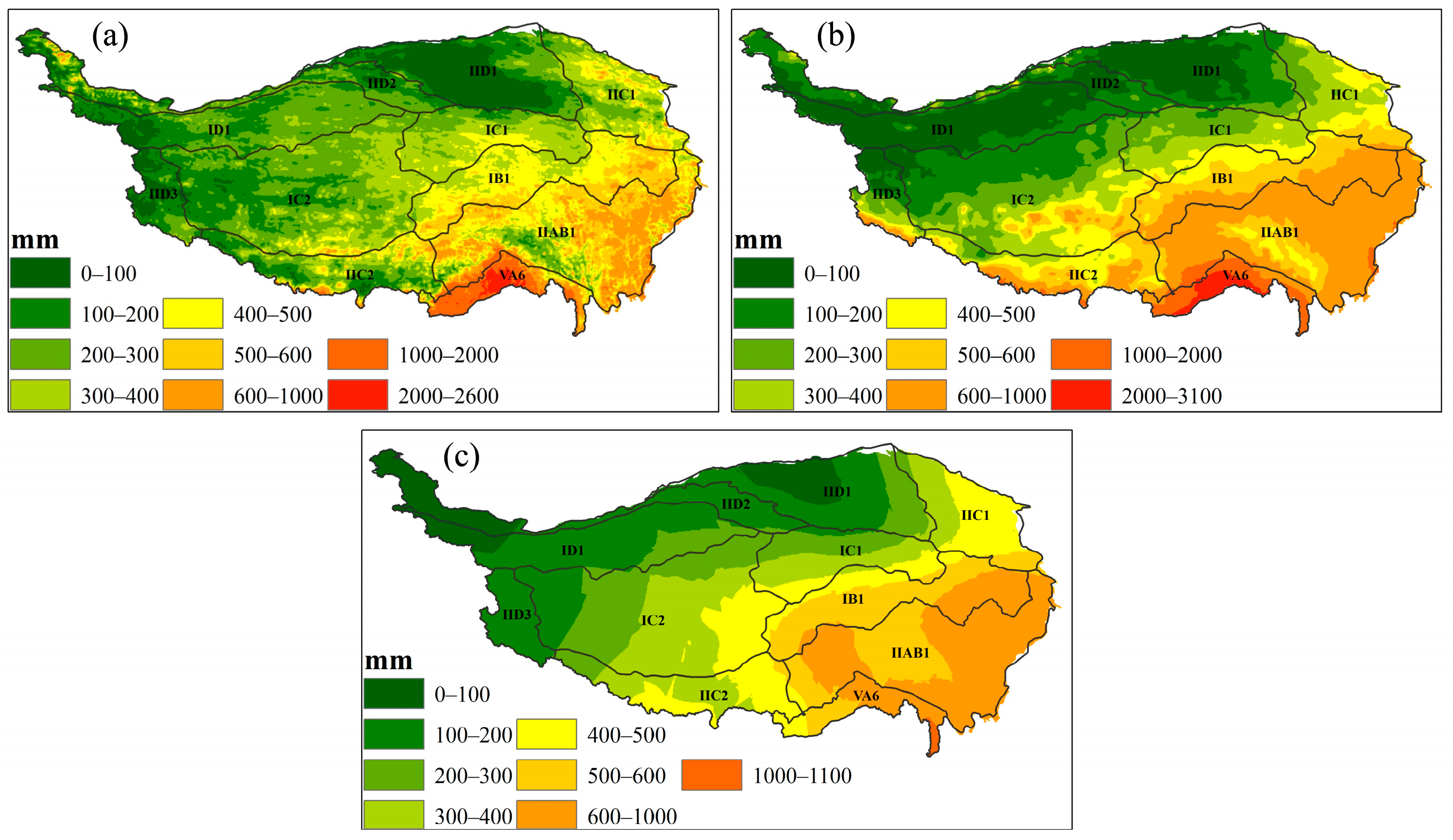
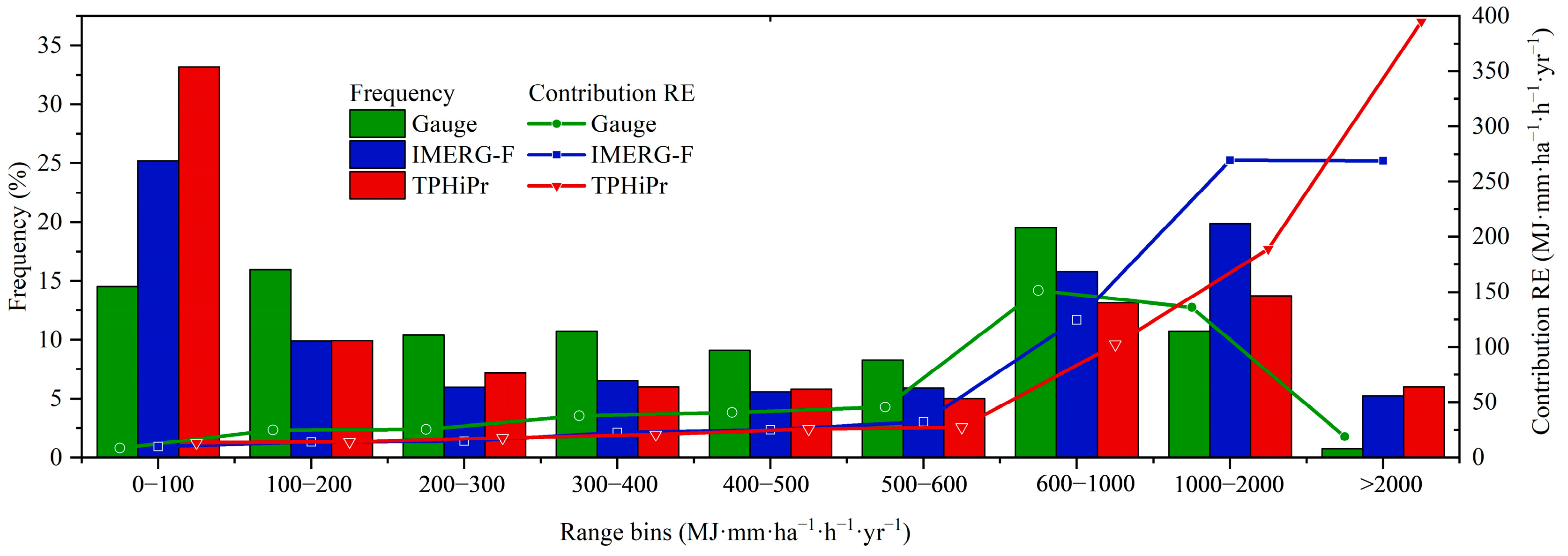
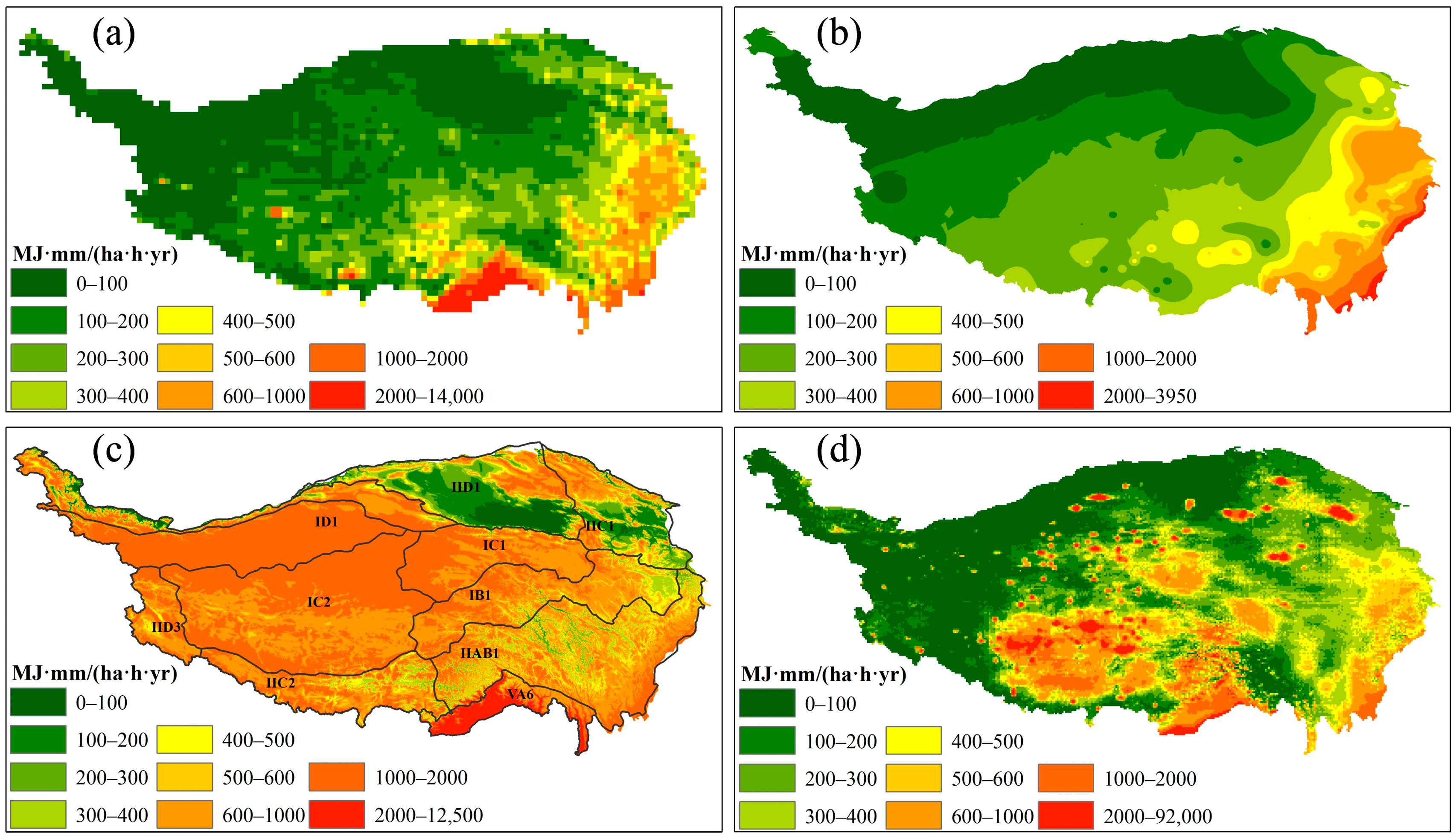
3.1. Spatial Distribution of Average Annual RE for Different Data Sources

Figure 3 shows the average annual RE and difference plot for the three data sources (TPHiPr, IMERG-F, and station data) from 2001 to 2020. In Figure 3, the spatial distribution of the average annual RE of the TPHiPr, IMERG-F and stations all showed increasing trends from northwest to southeast. The average annual RE are 806, 788, 490 MJ·mm·ha⁻¹·h⁻¹·yr^−1. The areas with an average annual RE less than 400 MJ·mm·ha⁻¹·h⁻¹·yr⁻¹ are mainly located in the high–cold desert, desert, and high–cold steppe zones (ID1, IID1, IID2, IID3, IC1, and IC2) in the northwest. Most of the eastern part of the study area had an average annual RE of 600–3000 MJ·mm·ha⁻¹·h⁻¹·yr⁻¹. The zone with the highest average annual RE was VA6, which is low in elevation and has a subtropical climate, with annual rainfall of up to 4000 mm. The results of the interpolation of station data interpolation (Figure 3c) show a strong band in the western and northern areas, which have a maximum RE of 3500 MJ·mm·ha⁻¹·h⁻¹·yr⁻¹. The grid data show low-value areas in the west and north of the TP, with no banding, and a high-value area in zone VA6; the maximum IMERG-F value is 18,000 MJ·mm·ha⁻¹·h⁻¹·yr⁻¹, and the maximum TPHiPr value is 31,000 MJ·mm·ha⁻¹·h⁻¹·yr⁻¹. The station-observed values were substantially lower, mainly between 200 and 2000 MJ·mm·ha⁻¹·h⁻¹·yr⁻¹. The largest difference in R values between the three data sources was identified for zone VA6. Compared with the IMERG-F results (Figure 3d), the TPHiPr average annual RE values were considerably higher in the central and western areas of zone VA6, with a difference of more than 3000 MJ·mm·ha⁻¹·h⁻¹·yr⁻¹. In the Great Lakes area of northern Tibet (IC2), the TPHiPr results were considerably lower than the IMERG-F results, and the TPHiPr results were closer to the station data, whereas the IMERG-F results were generally higher.

Table 2. Statistical values of different RE product zones (stations). Unit: MJ·mm·ha⁻¹·h⁻¹·yr⁻¹.

Zone	Gauge			IMERG-F			TPHiPr
	Min	Max	Mean	Min	Max	Mean	Min	Max	Mean
TP	8	3534	775	4	3655	1028	10	4280	883
VA6	1186	3534	2591	1837	3655	2977	1307	4280	2884
IIAB1	249	2065	1035	602	2593	1398	277	2713	1182
IB1	351	1254	744	470	1950	1068	410	1517	892
IIC2	320	1125	643	500	2477	1025	286	1407	715
IIC1	255	1154	658	213	1622	700	295	1154	736
IC2	288	553	413	478	1129	841	243	576	398
IC1	288	361	314	360	677	501	412	522	462
IID1	8	294	112	5	256	93	10	326	125
IID2	42	42	42	4	4	4	43	43	43
IID3	53	211	132	50	1245	647	58	404	231
ID1	/	/	/	/	/	/	/	/	/

presents statistics on the average annual RE within the different geographic zones. Regarding the mean values, both the TPHiPr results and IMERG-F calculations indicate an overestimation of average annual RE on the TP, with an overestimation of 13.6% and 32.6%. From the natural zone, IMERG-F results are lower than those of the station results in zones IID1 and IID2. The mean values of the results calculated from the gridded data were higher than those of the station results in other zones, where the TPHiPr results were closer to the station calculations.

Figure 4 shows the distribution of the different categories of average annual RE and their proportion of annual RE. The highest category of >2000 MJ·mm·ha⁻¹·h⁻¹·yr⁻¹ of station-calculated average annual RE was the least frequent, accounting for approximately 0.7% of all stations. The frequency of appearances of the other categories ranged from 8.3% to 19.5%, with the interval 600–1000 MJ·mm·ha⁻¹·h⁻¹·yr⁻¹ accounting for the highest proportion. The average annual RE distribution categories for TPHiPr and IMERG-F were similar, with the largest differences found in the intervals 0–100 MJ·mm·ha⁻¹·h⁻¹·yr⁻¹ and 1000–2000 MJ·mm·ha⁻¹·h⁻¹·yr⁻¹. The most frequent TPHiPr RE was the lowest category (0–100 MJ·mm·ha⁻¹·h⁻¹·year⁻¹), accounting for up to 33.2% of the total. The most frequent IMERG-F RE was also the lowest category, at approximately 25.2%. The proportion of the second highest category (1000–2000 MJ·mm·ha⁻¹·h⁻¹·yr⁻¹) was larger in the IMERG-F results than in the TPHiPr results. In all other categories, the differences in the proportions were minor. Regarding the size of the contribution to average annual RE of the first six categories, the differences between the contributions of the three data sources were small, but the station data provided slightly higher values. In the 6000–1000 MJ·mm·ha⁻¹·h⁻¹·yr⁻¹ contribution category, the RE contribution quantity was substantially larger, and the order was as follows: stations > IMERG-F > TPHiPr. The order of contributions in the second largest category was IMERG-F > TPHiPr > stations. In the largest category, the contribution of the stations was considerably lower, that of TPHiPr considerably increased to become the highest in this category, and that of IMERG-F did not change much from the previous category.

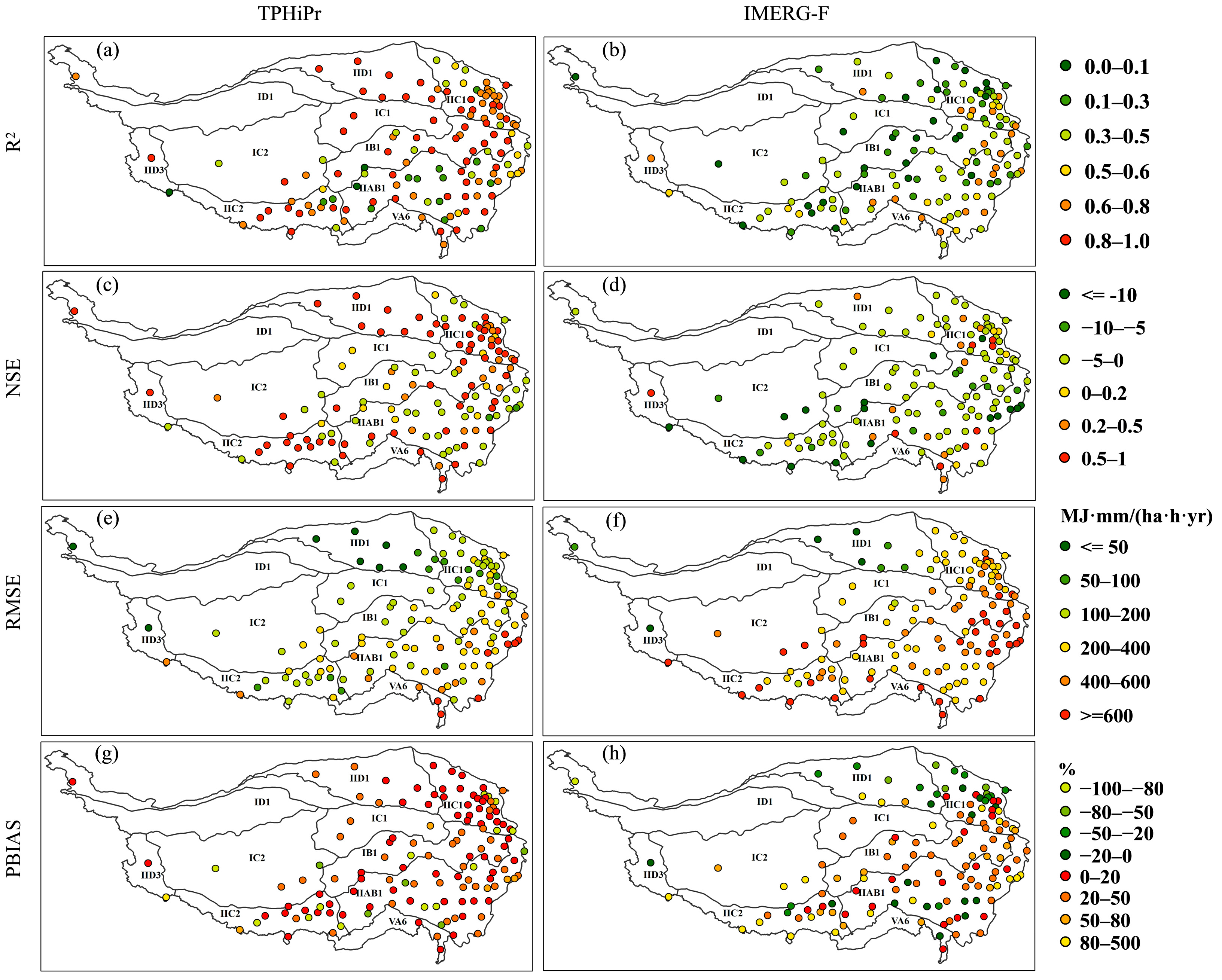
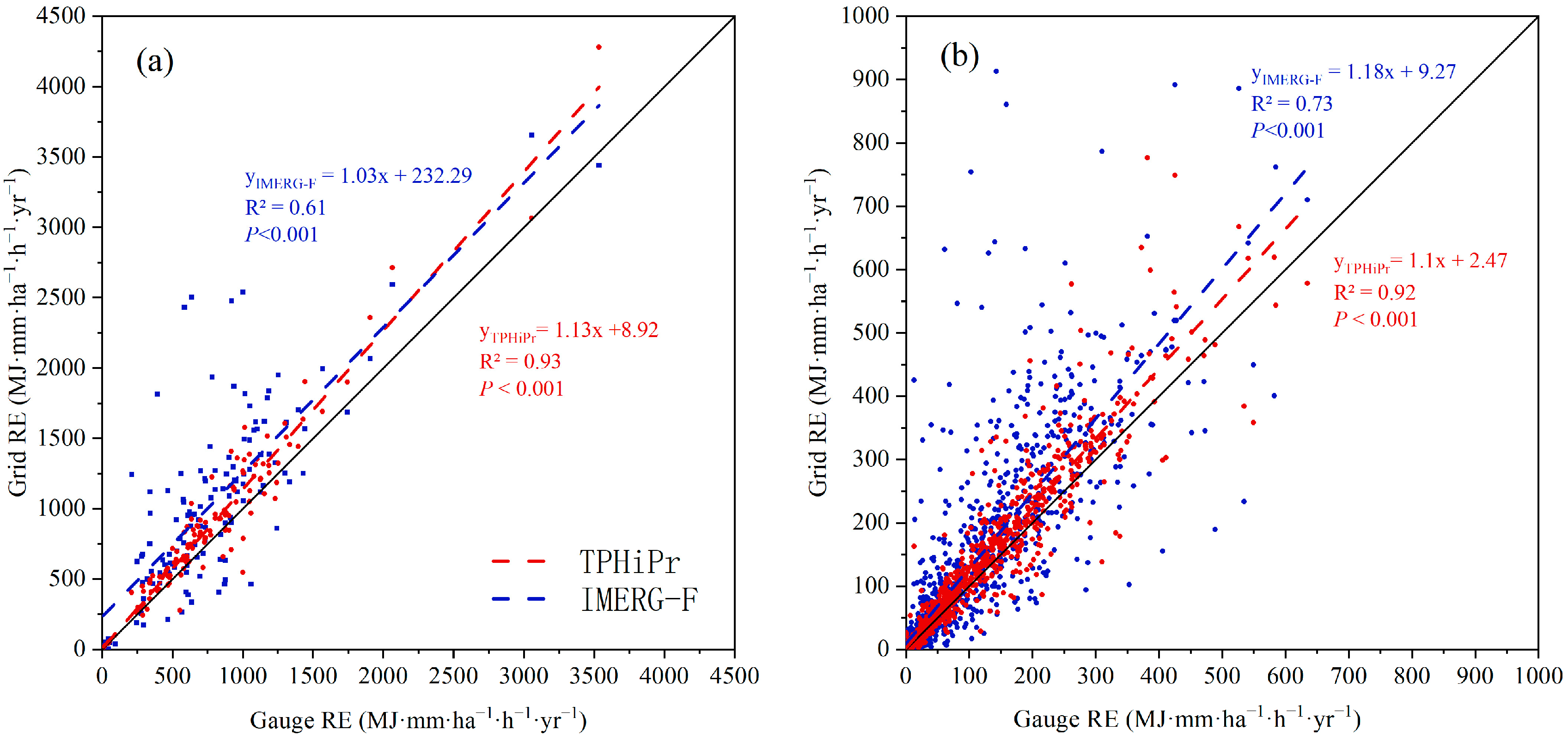
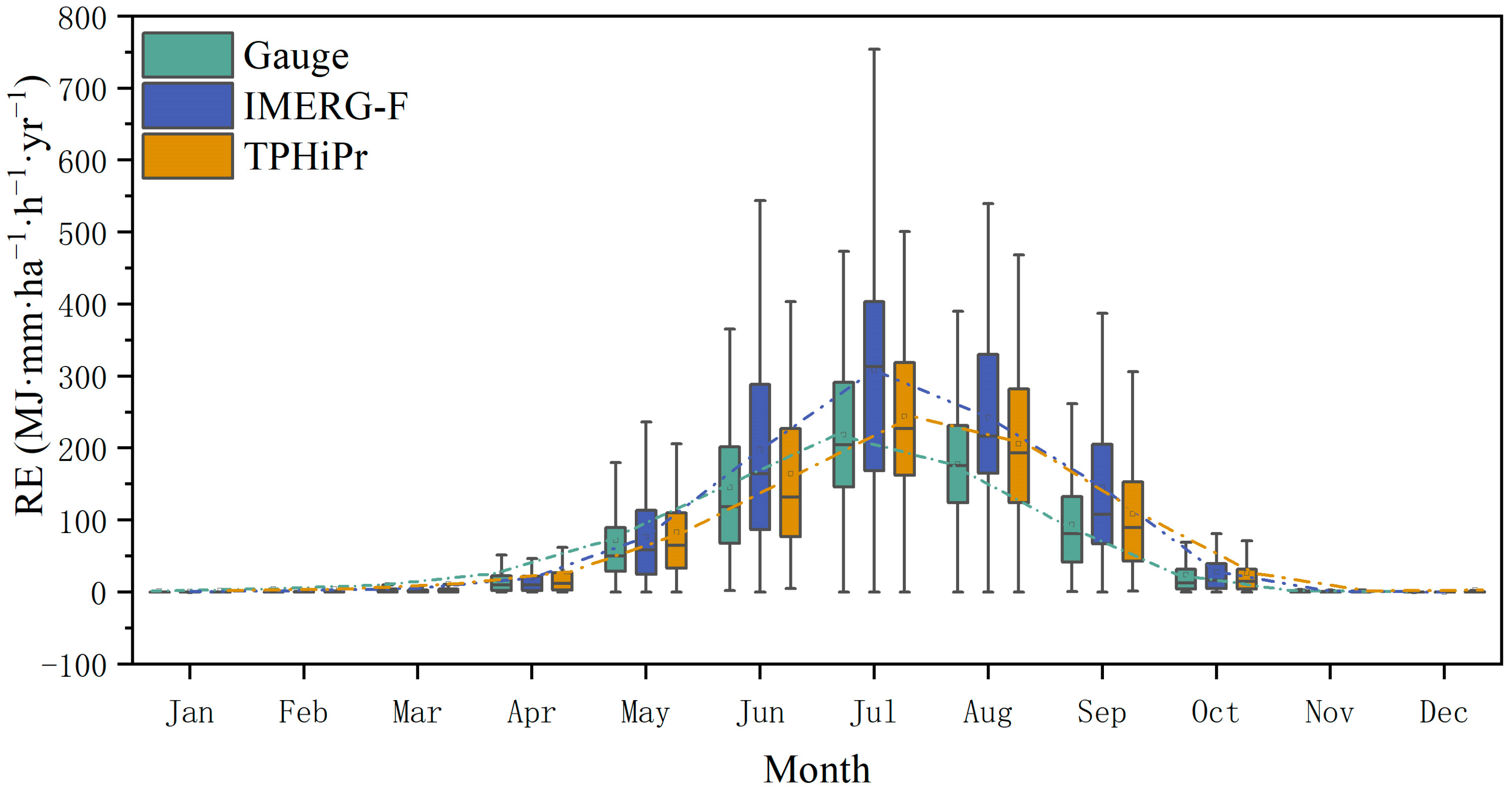
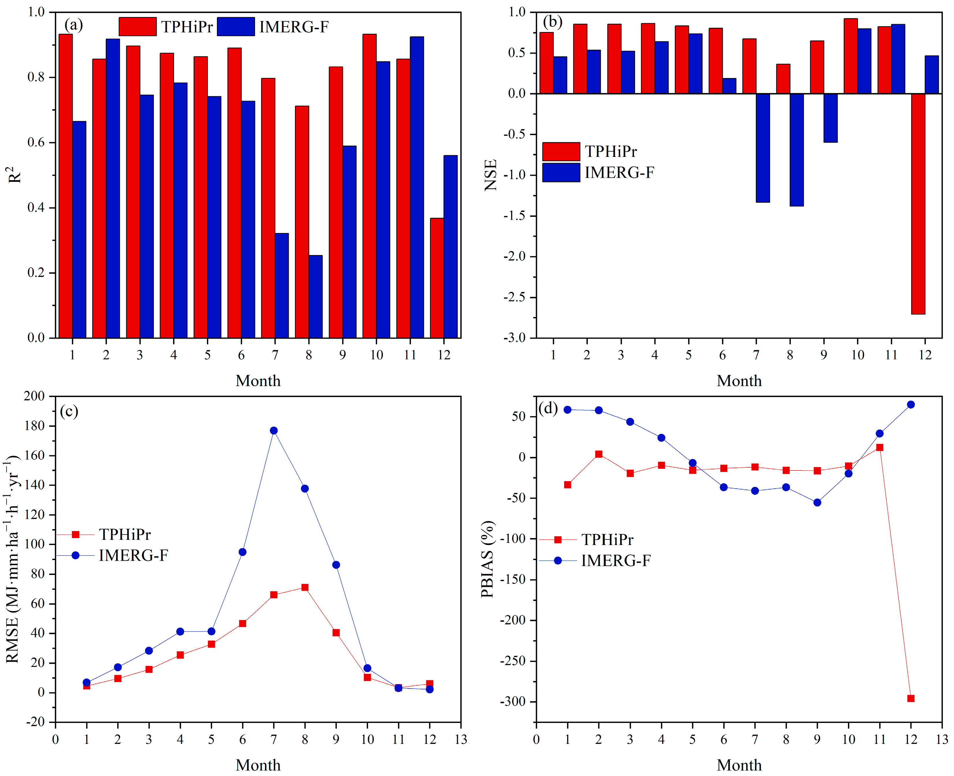
3.2. Evaluation of RE Accuracy at Station Scale

Compared with the station data (Figure 5), the differences range between TPHiPr and the station results was between −450 and 700 MJ·mm·ha⁻¹·h⁻¹·yr⁻¹, while the difference range with IMERG-F was between −600 and 1900 MJ·mm·ha⁻¹·h⁻¹·yr⁻¹. IMERG-F shows a larger difference amplitude. The gridded data contained overestimates, to varying degrees, along the southeastern boundary and some underestimates in the Hengduan Mountains. The TPHiPr results mostly overestimated RE, with values ranging from 0 to 200 MJ·mm·ha⁻¹·h⁻¹·yr⁻¹. We identified some underestimates in the vicinity of the Lhasa River south of the GDM. The IMERG-F results contained marked overestimates in the east and southwest, with the highest overestimates in the range of 1400–1900 MJ·mm·ha⁻¹·h⁻¹·yr⁻¹, as well as serious underestimates in the north, ranging from –600 to –400 MJ·mm·ha⁻¹·h⁻¹·yr⁻¹. The main reason for this difference is that there are few or no station data in the northern and western regions, resulting in low gridded data accuracy. Figure 5a,b show that on both sides of the middle reaches of the Yarlung Tsangpo River, the differences between the TPHiPr and station results were small, but the fluctuations in the differences between the IMERG-F and station results were large. At the boundary between IC2 and IIC2, located on the south side of the Yarlung Tsangpo River and the north side of the GDM, a narrow transition zone of elevated value differences was identified. The TPHiPr values, which contained slight overestimates, were closer to the station values, whereas the IMERG-F values contained notable underestimates. In zone IIC1, south of the QLM, the TPHiPr values were considerably higher than the IMERG-F values. The TPHiPr values, which contained slight overestimates, were closer to the station values, whereas the IMERG-F values contained significant underestimates. From the above, the TPHiPr results were closer to station-measured values, but with slight overestimations, and the results were more accurate than the IMERG-F results. In the Great Lakes region, the IMERG-F values were much higher than the TPHiPr values, with substantial overestimations.

The values of the four evaluation metrics (R², NSE, RMSE, and PBIAS) for annual RE for TPHiPr and IMERG-F at each station are shown in Figure 6. The R² of the annual RE between TPHiPr and the station exceeds 0.7 at 77 (58.8%) of the 131 stations. The number of stations with R² > 0.7 was only 6 (4.6%) for the IMERG-F. The R² values of the annual RE calculated using the two types of gridded data and by the stations were lower on the south side of the QLM; the correlation of the TPHiPr results in the rest of the region was stronger, whereas the correlation of the IMERG-F results was weaker in the northern, central, and southern parts of the region. The spatial variation in the NSE of both data types was similar to the variation in R², with low NSE values in the eastern region and the Hengduan Mountains. The mean RMSE values of the TPHiPr was 246 MJ·mm·ha⁻¹·h⁻¹·yr⁻¹, while the mean RMSE of the IMERG-F was 490 MJ·mm·ha⁻¹·h⁻¹·yr⁻¹. The RMSE values of the TPHiPr results were substantially lower than those of the IMERG-F results, with areas of high RMSE mainly distributed in the eastern and southern areas. The range of PBIAS values for the IMERG-F results (−90–50%) was larger than that of the TPHiPr results (−490–90%), with negative values mainly found in the north and larger positive values mainly found in the HLM and GDM in the eastern and southern areas.

Figure 7 depicts a comparison of the RE determined using TPHiPr and IMERG-F data with station-calculated precipitation. To ensure a more accurate comparison, 131 grid pixels were used to calculate the statistical indicators, and the results of the evaluation indices are shown in

Table 3. Statistical indicators of annual and monthly RE for different precipitation data.

Dataset	Time	R2	NSE	RMSE (MJ·mm·ha−1·h−1·yr−1)	SD (MJ·mm·ha−1·h−1·yr−1)	RMSE/SD	PBIAS (%)
Gauge	Year	/	/	/	499.27	/	/
TPHiPr		0.93	0.85	195.84	/	0.39	14.03
IMERG-F		0.61	0.07	481.19	/	0.96	32.77
Gauge	Month	/	/	/	90.09	/	/
TPHiPr		0.92	0.87	35.89	/	0.40	14.03
IMERG-F		0.73	0.39	77.22	/	0.86	32.77

. For TPHiPr and IMERG-F, the R² of the mean annual RE was 0.93 and 0.61, NSE was 0.85 and 0.07, RMSE was 195.84 and 481.19 MJ·mm·ha⁻¹·h⁻¹·yr⁻¹, and PBIAS was 14.03% and 32.77%; the R² of the mean monthly RE was 0.92 and 0.73, NSE was 0.87 and 0.39, RMSE was 35.89 and 77.22 MJ·mm·ha⁻¹·h⁻¹·yr⁻¹, and PBIAS was 14.03% and 32.77%, respectively. Overall, the TPHiPr mean annual/monthly RE more strongly correlated with the station data and PBIAS was lower. The RMSE/SD (Standard Deviation) values of TPHiPr were both less than 0.65, meaning that the predictions of TPHiPr are better than IMERG-F (RMSE/SD < 0.65 is considered low and acceptable [42,43,44]). Figure 7b shows a scatterplot of the monthly average RE calculated according to TPHiPr, IMERG-F, and station observations. Compared with the annual RE results, the RMSE of the monthly RE was lower, and the results were closer to the station data.

The monthly RE results are provided in Figure 8, which shows wide seasonal variation in RE in the study area. The erosive power of rainfall was mainly concentrated from May to September, reaching a maximum of 500 MJ·mm·ha⁻¹·h⁻¹·yr⁻¹ in July, with an average of 219 MJ·mm·ha⁻¹·h⁻¹·yr⁻¹. The lowest RE mainly occurred in November–March, with an average value of almost zero. Both TPHiPr and IMERG-F overestimated monthly RE, to a larger extent by the latter.

The results of the comparison between TPHiPr, IMERG-F, and station-observed monthly RE are shown in Figure 9. Except for December, the R² of the monthly RE of TPHiPr ranged from 0.71 to 0.93, with a mean value above 0.85, indicating that the TPHiPr precipitation product can accurately capture the characteristics of the changes in monthly RE; the NSE indicator and R² performed similarly, but their values were susceptible to anomalies in December due to the low precipitation amount. The R² of IMERG-F ranged from 0.25 to 0.93, with values of 0.32, 0.25, and 0.59 in July, August, and September, respectively. The RE from July to September accounted for a large proportion of the annual total, indicating that IMERG-F does not capture high RE conditions well.

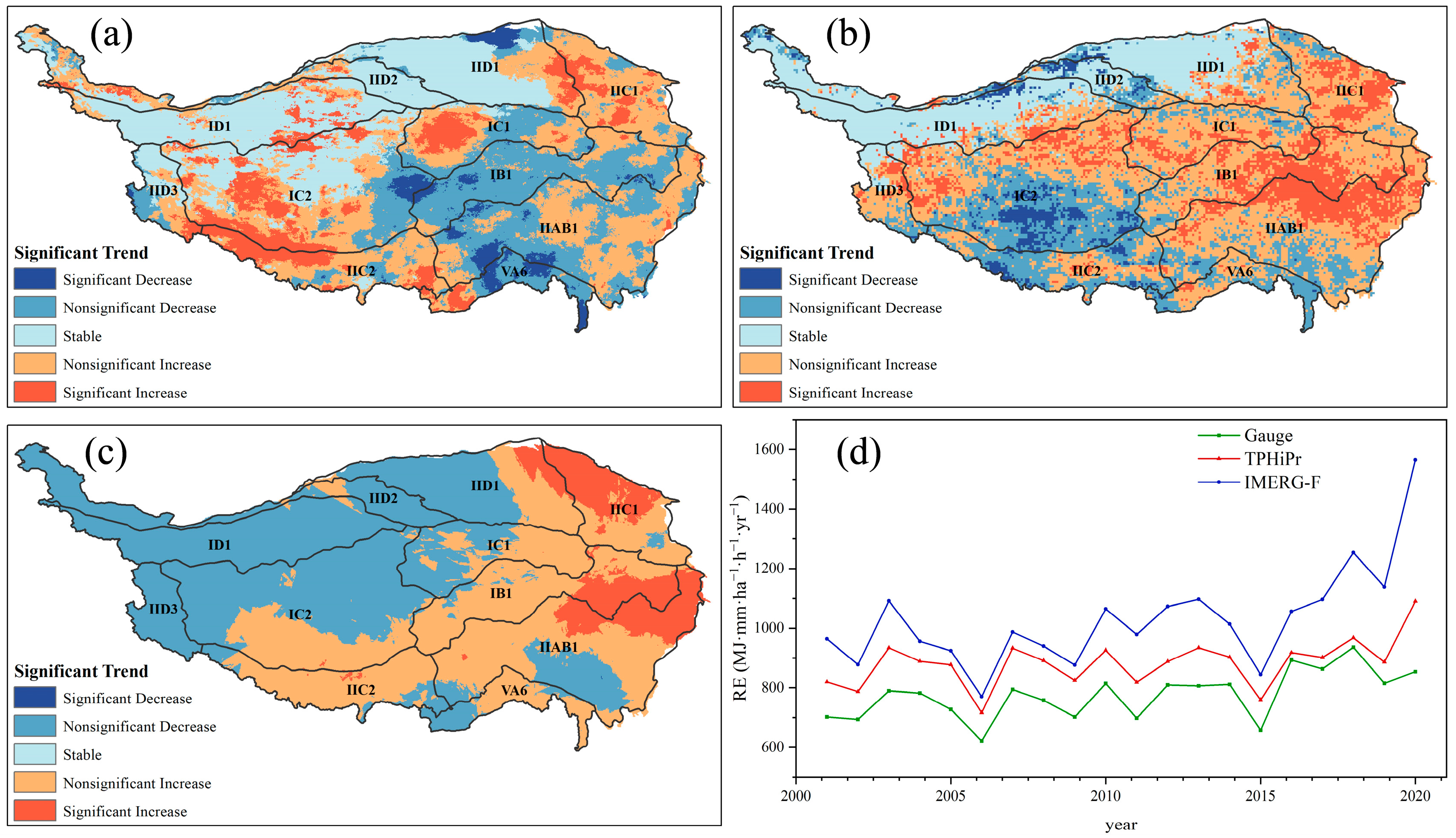
3.3. Comparison of RE Trends on the TP

Table 4. Significance trend area ratios for different data sources.

Significance Trend	Gauge (%)	IMERG-F (%)	TPHiPr (%)
Significant Decrease	0.00	4.00	0.32
Nonsignificant Decrease	49.24	22.16	16.21
Stable	0.00	17.30	17.36
Nonsignificant Increase	40.03	40.15	45.37
Significant Increase	10.73	16.39	20.74

shows remarkable differences in the changes in RE between the station data and gridded data, with the two types of gridded data having similar significance regarding trend area ratios but with different regions showing changes. The distributions of the annual RE and significance trend changes from 2001 to 2020 for station-interpolated, IMERG-F, and TPHiPr data are depicted in Figure 10. Figure 10a shows an overall increasing trend in the TPHiPr annual RE. Areas with increasing RE accounted for 66.11% of the total annual RE, while areas with significantly increasing RE constituted 20.74%, primarily in zone IC2; areas with decreasing RE were mainly in the Hengduan Mountains and on either side of the NQM, accounting for 16.53% of the erosivity, with areas experiencing a significant decrease in RE accounting for 0.32% of the total annual RE. Stable areas were mainly located in the northwest, accounting for 17.36% of the total. Figure 10b shows that areas of decreasing annual RE in the IMERG-F results were mainly distributed in the Great Lakes region and along the Yarlung Tsangpo River, accounting for 26.17% of the region, with areas experiencing significant decreases accounting for 4% of the total, mainly in the Great Lakes region and near the ALM. Stable areas were mainly in the northwest, accounting for 17.3%; areas with increases were mainly located in the southeast and along the TGM in the central part of the region, accounting for 56.53%. Areas with significant increases in RE were mainly distributed in the east and accounted for 16.39%. Figure 10c shows that the decreasing annual RE in the station results was mainly occurring in the northwest as well as the southern part of zone IIAB1, accounting for 49.24% of the region, with no areas experiencing significant decreases. Areas experiencing increases were mainly located in the southeast, accounting for 50.76% of the whole region, with 10.72% experiencing significant increases. The areas of significant increases were mainly distributed in the southern QLM and the boundary between IB1 and IIAB1. Figure 10d shows that the annual RE determined using the three types of precipitation data showed fluctuating changes from 2001 to 2015. The results calculated using the gridded data were slightly high, with the IMERG-F results showing the largest differences from the station-measured results. The change trend of the gridded data is completely consistent with the site data, because both gridded data integrate site data; however, there are significant differences in special distribution. The regions with the greatest differences are in IB1 and the southwest region. The calculation result of TPHiPr in the IB1 area is opposite to others, indicating a significant decrease, while the results of IMERG-F in the southwestern region are opposite to other results, indicating a significant decrease.

4. Discussion

The spatial distribution of precipitation on the TP exhibits a pattern of decreasing from southeast to northwest [45,46]. The terrain is complex, characterized by alternating mountain ranges and basins. In the arid and semiarid regions of the northwestern TP, there is a lower density of meteorological stations, while in the southeastern part, the density of meteorological stations is higher. During the interpolation of station-based RE to create RE map, the values in the northwest region tend to be overestimated, failing to accurately represent the differences in RE caused by the terrain. The gridded data show the geographical variation in the mountainous and basin areas, with a strong correlation with topography, especially around the HLM, NQM, GDM, and the Great Lakes area. The complex plateau topography, with its many gullies and ravines, can increase water vapor transport channels, which can increase regional net water vapor input [47,48,49]. The Hengduan Mountains are composed of several north–south-aligned mountain ranges, and water vapor arising in the south can cause strong precipitation in the north–south direction. The TPHiPr values are higher in this area, with some internal differences, which reflect the differences between mountain ranges and valleys, to an extent. Observation stations were selected using the U.S. National Climatic Data Center’s (NCDC) Global Historical Climatology Network–Daily (GHCN–Daily). Twenty years of valid precipitation data were used as the selection indicator. Two stations were ultimately selected in the area, as indicated in Figure 1. The time series of daily precipitation data of Station 1 spanned the period of 1918 to 1970, for a total of 41 valid years. The average annual RE was calculated as 38,765 MJ·mm·ha⁻¹·h⁻¹·yr⁻¹ using the daily erosion model. The time series of daily precipitation of Station 2 covered 1929–1948, for a total of 20 valid years, and the average annual RE was calculated as 42,095 MJ·mm·ha⁻¹·h⁻¹·yr⁻¹ using the daily erosion model. The average annual RE of the two stations was 40,430 MJ·mm·ha⁻¹·h⁻¹·yr⁻¹, which is closer to that of TPHiPr. A narrow rain shadow zone is present on the north side of the HLM [50], and the TPHiPr results show higher R values on the windward slopes of the HLM as well as on the south side of the NQM and GDM, as well as lower R values on the north side in the rain shadow. However, the R values of the IMERG-F results are not heterogeneous in these areas. The TPHiPr results are higher than those of IMERG-F on the south side of the QLM, which is a region with relatively high precipitation on the windward slopes. The TPHiPr results are closer to the station data, while the IMERG-F results are lower. The number of stations is higher in zones IIC1, IIAB1, and IB1, which are mainly in the HLM and Hengduan Mountains, but the large number of mountain ranges and the highly varied topography increase the spatial differences in precipitation. Moreover, stations are mainly located at lower elevations, so they do not reflect the precipitation of the whole area. In areas where the influence of terrain is not considered in gridded data and station data correction is insufficient, the results show considerable deviations.

The results of the RE on the TP with previous research calculated using different precipitation data sources are listed in

Table 5. Average annual RE results from current and previous studies.

Study Area	Precipitation Data Source	No. Station	Time Resolution	Spatial Resolution	Calculation Method	Spatial Method	Max. RE	Avg. RE	Reference
TP	Weather stations, ERA5	1787	1 min, hour	0.25°	Standard	Proportional IDW interpolation correction	13,947	290	Chen et al. [27]
China	Weather stations	2381	Hourly	1 km	Standard	Universal kriging	3906	288	Yue et al. [18]
Global	Precipitation stations	3540	Hourly and sub-hourly	30 arc seconds	Standard	Gaussian process regression	12,347	980	Panagos et al. [17]
Global	CMORPH		30 min	8 km	Standard	Generic correction linear	91,746	440	Bezak et al. [22]
TP	Weather stations	131	Daily	1/30°	Experience	Ordinary kriging	3521	490	This study
TP	TPHiPr		Daily	1/30°	Experience		30,685	806	This study
TP	IMERG-F		Daily	0.1°	Experience		18,203	787	This study

and Figure 11. In this study, the calculated mean RE using meteorological station data is 490 MJ·mm·ha⁻¹·h⁻¹·yr⁻¹, which is higher than the results from Yue et al. [18] and Chen et al. [27], whose mean RE is around 290 MJ·mm·ha⁻¹·h⁻¹·yr⁻¹. This value is lower than that reported by Panagos et al. [17], who used global precipitation station data to calculate an RE average of 980 MJ·mm·ha⁻¹·h⁻¹·yr⁻¹. Previous studies have indicated that calculating RE using daily precipitation data from meteorological stations tends to result in higher values compared to calculations based on hourly or minute data [18]. As shown in Figure 11a, areas with a higher density of meteorological stations in the southeast exhibit better results. However, the full-coverage grid used low resolution and spatial accuracy, with a resolution of 0.25°. It is challenging to adequately capture the spatial variations in RE caused by the terrain differences on the TP. Figure 11b, which was produced using the universal kriging, shows an overall decreasing trend from east to west, with insignificant changes among the contours. Unlike the other results, VA6 is a low-value area. Panagos incorporated data from high-erosivity stations around the TP, resulting in the overall outcome showing a high range of values (Figure 11c). In this study, the calculated average RE values using two grid datasets were around 800 MJ·mm·ha⁻¹·h⁻¹·yr⁻¹. Bezak et al. [22] reported a maximum value of 91,746 MJ·mm·ha⁻¹·h⁻¹·yr⁻¹ and an average of 440 MJ·mm·ha⁻¹·h⁻¹·yr⁻¹ calculated using global CMORPH data source. In Figure 11d, a significant high-value area is observed in the southwest region, with scattered high-value areas predominantly over water bodies, which suggests that CMORPH judges lakes to be high-value areas for precipitation.

When only station data are used for the TP region, the results are highly dependent on the number and distribution of stations, and ensuring the accuracy of the results in areas with no stations or low station density is difficult. For the RE calculated using only gridded data, larger discrepancies were found between the results and known precipitation and topographic features. As a high-density station and grid-merged precipitation dataset, TPHiPr has a higher resolution and can relatively accurately reflect the influence of mountain ranges with an east–west alignment on precipitation on the TP (i.e., windward slopes and rain shadow areas) as well as the high-value areas of RE in the north–south-aligned Hengduan Mountains.

5. Conclusions

In this study, a daily rainfall erosion model fitted using sinusoidal seasonal variation curves was used to calculate the RE on the TP using two gridded precipitation datasets (TPHiPr and IMERG-F) and the data from 131 weather stations. Our comparison of the RE among the station observations and the gridded precipitation data revealed the following: Both TPHiPr and IMERG-F overestimate RE compared with station observations, with IMERG-F overestimates being more pronounced for areas mainly located in the eastern and southern parts of the study area. The accuracy of average annual RE calculated using gridded precipitation data is lower than that calculated using monthly average RE. The statistical indicators of both annual and monthly average RE calculated using TPHiPr data are better than those for the IMERG-F data, with around 0.9 for R² and NSE. The spatial distribution of the average annual RE calculated using TPHiPr data more accurately reflects the actual data on the TP. TPHiPr effectively reveals rain shadow areas on the northern slopes of the Himalayas and calculates RE more accurately in the broad-leaved evergreen forest zone on the southern flank of HLM and the arid regions to the northwest. The analysis of the trends in the annual RE using the three types of precipitation data indicated that RE on the TP fluctuated between 2000 and 2015 and trended upward after 2015; RE during the period from 2001 to 2020 showed an overall increasing trend, accounting for 66.11% of the total period, with a significant increase contributing to 20.74%.

Compared with the results of other studies, TPHiPr can more accurately characterize the spatial and temporal characteristics of the changes in the rainfall on the TP region, but it produces underestimates in the southern valleys and the eastern Hengduan Mountains as well as overestimates in the southeastern area at lower elevations. Therefore, when using these data, the precipitation data should be optimized according to the specific study area, considering both topography and vegetation characteristics to reduce the uncertainty in the results.

References

1. Smith, P.; House, J.I.; Bustamante, M.; Kuikman, P.; Pugh, T.A.M. Global change pressures on soils from land use and management. Glob. Chang. Biol. 2016, 22, 1008–1028. [Google Scholar] [CrossRef] [PubMed]
2. Wuepper, D.; Borrelli, P.; Finger, R. Countries and the global rate of soil erosion. Nat. Sustain. 2020, 3, 51–55. [Google Scholar] [CrossRef]
3. Panagos, P.; Ballabio, C.; Borrelli, P.; Meusburger, K.; Klik, A.; Rousseva, S.; Tadić, M.P.; Michaelides, S.; Hrabalíková, M.; Olsen, P.; et al. Rainfall erosivity in Europe. Sci. Total Environ. 2015, 511, 801–814. [Google Scholar] [CrossRef]
4. Nearing, M.A.; Yin, S.-q.; Borrelli, P.; Polyakov, V.O. Rainfall erosivity: An historical review. Catena 2017, 157, 357–362. [Google Scholar] [CrossRef]
5. Wischmeier, W.H.; Smith, D.D. Rainfall energy and its relationship to soil loss. Eos Trans. Am. Geophys. Union 1958, 39, 285–291. [Google Scholar]
6. Renard, K.G. Predicting Soil Erosion by Water: A Guide to Conservation Planning with the Revised Universal Soil Loss Equation (RUSLE); United States Government Printing: Washington, DC, USA, 1997.
7. Wischmeier, W.H.; Smith, D.D. Predicting Rainfall Erosion Losses: A Guide to Conservation Planning; Department of Agriculture, Science and Education Administration: Washington, DC, USA, 1978. [Google Scholar]
8. Margiorou, S.; Kastridis, A.; Sapountzis, M. Pre/Post-Fire Soil Erosion and Evaluation of Check-Dams Effectiveness in Mediterranean Suburban Catchments Based on Field Measurements and Modeling. Land 2022, 11, 1705. [Google Scholar] [CrossRef]
9. Phinzi, K.; Ngetar, N.S. The assessment of water-borne erosion at catchment level using GIS-based RUSLE and remote sensing: A review. Int. Soil Water Conserv. Res. 2019, 7, 27–46. [Google Scholar] [CrossRef]
10. Xie, Y.; Yin, S.-q.; Liu, B.-y.; Nearing, M.A.; Zhao, Y. Models for estimating daily rainfall erosivity in China. J. Hydrol. 2016, 535, 547–558. [Google Scholar] [CrossRef]
11. Angulo-Martínez, M.; Beguería, S. Estimating rainfall erosivity from daily precipitation records: A comparison among methods using data from the Ebro Basin (NE Spain). J. Hydrol. 2009, 379, 111–121. [Google Scholar] [CrossRef]
12. Chen, Y.; Ding, M.; Zhang, G.; Duan, X.; Wang, C. The possible role of fused precipitation data in detection of the spatiotemporal pattern of rainfall erosivity over the Tibetan Plateau, China. Catena 2023, 228, 107114. [Google Scholar] [CrossRef]
13. Liu, B.; Xie, Y.; Li, Z.; Liang, Y.; Guo, Q. The assessment of soil loss by water erosion in China. Int. Soil Water Conserv. Res. 2020, 8, 430–439. [Google Scholar] [CrossRef]
14. Li, X.; Li, Z.; Lin, Y. Suitability of TRMM Products with Different Temporal Resolution (3-Hourly, Daily, and Monthly) for Rainfall Erosivity Estimation. Remote Sens. 2020, 12, 3924. [Google Scholar] [CrossRef]
15. Gu, Z.; Feng, D.; Duan, X.; Gong, K.; Li, Y.; Yue, T. Spatial and Temporal Patterns of Rainfall Erosivity in the Tibetan Plateau. Water 2020, 12, 200. [Google Scholar] [CrossRef]
16. Yin, S.; Xie, Y.; Liu, B.; Nearing, M.A. Rainfall erosivity estimation based on rainfall data collected over a range of temporal resolutions. Hydrol. Earth Syst. Sci. 2015, 19, 4113–4126. [Google Scholar] [CrossRef]
17. Panagos, P.; Borrelli, P.; Meusburger, K.; Yu, B.; Klik, A.; Jae Lim, K.; Yang, J.E.; Ni, J.; Miao, C.; Chattopadhyay, N. Global rainfall erosivity assessment based on high-temporal resolution rainfall records. Sci. Rep. 2017, 7, 4175. [Google Scholar] [CrossRef] [PubMed]
18. Yue, T.; Yin, S.; Xie, Y.; Yu, B.; Liu, B. Rainfall erosivity mapping over mainland China based on high-density hourly rainfall records. Earth Syst. Sci. Data 2022, 14, 665–682. [Google Scholar] [CrossRef]
19. Teng, H.F.; Liang, Z.Z.; Chen, S.C.; Liu, Y.; Rossel, R.A.V.; Chappell, A.; Yu, W.; Shi, Z. Current and future assessments of soil erosion by water on the Tibetan Plateau based on RUSLE and CMIP5 climate models. Sci. Total Environ. 2018, 635, 673–686. [Google Scholar] [CrossRef]
20. Das, S.; Jain, M.K.; Gupta, V. A step towards mapping rainfall erosivity for India using high-resolution GPM satellite rainfall products. Catena 2022, 212, 106067. [Google Scholar] [CrossRef]
21. Delgado, D.; Sadaoui, M.; Ludwig, W.; Méndez, W. Spatio-temporal assessment of rainfall erosivity in Ecuador based on RUSLE using satellite-based high frequency GPM-IMERG precipitation data. Catena 2022, 219, 106597. [Google Scholar] [CrossRef]
22. Bezak, N.; Borrelli, P.; Panagos, P. Exploring the possible role of satellite-based rainfall data in estimating inter- and intra-annual global rainfall erosivity. Hydrol. Earth Syst. Sci. 2022, 26, 1907–1924. [Google Scholar] [CrossRef]
23. Teng, H.; Ma, Z.; Chappell, A.; Shi, Z.; Liang, Z.; Yu, W. Improving Rainfall Erosivity Estimates Using Merged TRMM and Gauge Data. Remote Sens. 2017, 9, 1134. [Google Scholar] [CrossRef]
24. Tang, L.; Tian, Y.; Yan, F.; Habib, E. An improved procedure for the validation of satellite-based precipitation estimates. Atmos. Res. 2015, 163, 61–73. [Google Scholar] [CrossRef]
25. Wang, Y.; Cheng, C.; Xie, Y.; Liu, B.; Yin, S.; Liu, Y.; Hao, Y. Increasing trends in rainfall-runoff erosivity in the Source Region of the Three Rivers, 1961–2012. Sci. Total Environ. 2017, 592, 639–648. [Google Scholar] [CrossRef] [PubMed]
26. Wang, L.; Zhang, F.; Fu, S.H.; Shi, X.N.; Chen, Y.; Jagirani, M.D.; Zeng, C. Assessment of soil erosion risk and its response to climate change in the mid-Yarlung Tsangpo River region. Environ. Sci. Pollut. Res. 2020, 27, 607–621. [Google Scholar] [CrossRef] [PubMed]
27. Chen, Y.; Duan, X.; Ding, M.; Qi, W.; Wei, T.; Li, J.; Xie, Y. New gridded dataset of rainfall erosivity (1950–2020) on the Tibetan Plateau. Earth Syst. Sci. Data 2022, 14, 2681–2695. [Google Scholar] [CrossRef]
28. Chen, Y. Rainfall erosivity estimation over the Tibetan plateau based on high spatial-temporal resolution rainfall records. Int. Soil Water Conserv. Res. 2022, 10, 422–432. [Google Scholar] [CrossRef]
29. Huffman, G.J.; Bolvin, D.T.; Braithwaite, D.; Hsu, K.; Joyce, R.; Xie, P.; Yoo, S.-H. NASA global precipitation measurement (GPM) integrated multi-satellite retrievals for GPM (IMERG). Algorithm Theor. Basis Doc. (ATBD) Version 2015, 4, 30. [Google Scholar]
30. Xu, R.; Tian, F.Q.; Yang, L.; Hu, H.C.; Lu, H.; Hou, A.Z. Ground validation of GPM IMERG and TRMM 3B42V7 rainfall products over southern Tibetan Plateau based on a high-density rain gauge network. J. Geophys. Res.-Atmos. 2017, 122, 910–924. [Google Scholar] [CrossRef]
31. Lu, D.; Yong, B. Evaluation and Hydrological Utility of the Latest GPM IMERG V5 and GSMaP V7 Precipitation Products over the Tibetan Plateau. Remote Sens. 2018, 10, 2022. [Google Scholar] [CrossRef]
32. Chen, Y.; Xu, M.; Wang, Z.; Gao, P.; Lai, C. Applicability of two satellite-based precipitation products for assessing rainfall erosivity in China. Sci. Total Environ. 2021, 757, 143975. [Google Scholar] [CrossRef] [PubMed]
33. Jiang, Y.; Yang, K.; Qi, Y.; Zhou, X.; He, J.; Lu, H.; Li, X.; Chen, Y.; Li, X.; Zhou, B. TPHiPr: A long-term (1979–2020) high-accuracy precipitation dataset (1∕30°, daily) for the Third Pole region based on high-resolution atmospheric modeling and dense observations. Earth Syst. Sci. Data 2023, 15, 621–638. [Google Scholar] [CrossRef]
34. Li, G.; Yu, Z.; Wang, W.; Ju, Q.; Chen, X. Analysis of the spatial Distribution of precipitation and topography with GPM data in the Tibetan Plateau. Atmos. Res. 2021, 247, 105259. [Google Scholar] [CrossRef]
35. Zheng, D.; Zhao, D.S. Characteristics of natural environment of the Tibetan Plateau. Sci. Technol. Rev 2017, 35, 13–22. [Google Scholar]
36. Yang, K.; Jiang, Y. A Long-Term (1979–2020) High-Resolution (1/30°) Precipitation Dataset for the Third Polar Region (TPHiPr); N.T.P.D. Center, Ed.; National Tibetan Plateau Data Center: Beijing, China, 2022. [Google Scholar]
37. GES DISC. Available online: https://disc.gsfc.nasa.gov/ (accessed on 11 July 2021).
38. Nash, J.E.; Sutcliffe, J.V. River flow forecasting through conceptual models part I—A discussion of principles. J. Hydrol. 1970, 10, 282–290. [Google Scholar] [CrossRef]
39. Kendall, M.G. Rank Correlation Methods, 4th ed.; Charles Griffin: London, UK, 1975. [Google Scholar]
40. Mann, H.B. Nonparametric Tests Against Trend. Econometrica 1945, 13, 245–259. [Google Scholar] [CrossRef]
41. Sen, P.K. Estimates of the Regression Coefficient Based on Kendall’s Tau. J. Am. Stat. Assoc. 1968, 63, 1379–1389. [Google Scholar] [CrossRef]
42. Kastridis, A.; Theodosiou, G.; Fotiadis, G. Investigation of Flood Management and Mitigation Measures in Ungauged NATURA Protected Watersheds. Hydrology 2021, 8, 170. [Google Scholar] [CrossRef]
43. Moriasi, N.D.; Arnold, G.J.; Van Liew, W.M.; Bingner, L.R.; Harmel, D.R.; Veith, L.T. Model Evaluation Guidelines for Systematic Quantification of Accuracy in Watershed Simulations. Trans. ASABE 2007, 50, 885–900. [Google Scholar] [CrossRef]
44. Singh, J.; Knapp, H.V.; Arnold, J.; Demissie, M. Hydrological modeling of the Iroquois river watershed using HSPF and SWAT 1. JAWRA J. Am. Water Resour. Assoc. 2005, 41, 343–360. [Google Scholar] [CrossRef]
45. Wang, Y.; Kong, Y.; Chen, H.; Zhao, L. Improving daily precipitation estimates for the Qinghai-Tibetan plateau based on environmental similarity. Int. J. Climatol. 2020, 40, 5368–5388. [Google Scholar] [CrossRef]
46. Ma, Z.; Xu, Y.; Peng, J.; Chen, Q.; Wan, D.; He, K.; Shi, Z.; Li, H. Spatial and temporal precipitation patterns characterized by TRMM TMPA over the Qinghai-Tibetan plateau and surroundings. Int. J. Remote Sens. 2018, 39, 3891–3907. [Google Scholar] [CrossRef]
47. Li, G.; Chen, H.; Xu, M.; Zhao, C.; Zhong, L.; Li, R.; Fu, Y.; Gao, Y. Impacts of Topographic Complexity on Modeling Moisture Transport and Precipitation over the Tibetan Plateau in Summer. Adv. Atmos. Sci. 2022, 39, 1151–1166. [Google Scholar] [CrossRef]
48. Lin, C.; Chen, D.; Yang, K.; Ou, T. Impact of model resolution on simulating the water vapor transport through the central Himalayas: Implication for models’ wet bias over the Tibetan Plateau. Clim. Dyn. 2018, 51, 3195–3207. [Google Scholar] [CrossRef]
49. Xu, K.; Zhong, L.; Ma, Y.; Zou, M.; Huang, Z. A study on the water vapor transport trend and water vapor source of the Tibetan Plateau. Theor. Appl. Climatol. 2020, 140, 1031–1042. [Google Scholar] [CrossRef]
50. Wang, Y.; Yang, K.; Zhou, X.; Wang, B.; Chen, D.; Lu, H.; Lin, C.; Zhang, F. The Formation of a Dry-Belt in the North Side of Central Himalaya Mountains. Geophys. Res. Lett. 2019, 46, 2993–3000. [Google Scholar] [CrossRef]
Figure 1. Map of TP and locations of weather stations. ① Himalaya Mountains, ② Hengduan Mountains, ③ Nyainqentanglha Mountains, ④ Gandist Mountains, ⑤ Tangula Mountains, ⑥ Kunlun Mountains, ⑦ Altun Mountains, ⑧ Qilian Mountains; For explanations of zone labels, please see Table 1.
Remotesensing 15 05267 g001
Figure 2. Average annual rainfall for 2001–2020: (a) TPHiPr, (b) IMERG-F, and (c) weather stations.
Remotesensing 15 05267 g002
Figure 3. Average annual RE for 2001–2020: (a) TPHiPr, (b) IMERG-F, and (c) weather stations. (d) Differences in average annual RE of TPHiPr and IMERG-F.
Remotesensing 15 05267 g003
Figure 4. Histogram of annual RE values in different categories and their contribution dot line plot to annual RE.
Remotesensing 15 05267 g004
Figure 5. Average annual RE differences for 2001–2020 between (a) TPHiPr and station-observed values and (b) IMERG-F and station-observed values.
Remotesensing 15 05267 g005
Figure 6. Spatial distribution of (a,b) R2; (c,d) Nash–Sutcliffe efficiency (NSE); (e,f) root mean square error (RMSE); (g,h) PBIAS between observed yearly RE and grid precipitation yearly values estimated using two types of data during 2001–2020 at 131 grid points.
Remotesensing 15 05267 g006
Figure 7. Scatterplots of RE of TPHiPr, IMERG-F, and station observations: (a) annual and (b) monthly mean RE.
Remotesensing 15 05267 g007
Figure 8. Comparison of monthly erosivity from different sources of rainfall data.
Remotesensing 15 05267 g008
Figure 9. Monthly changes in (a) R2, (b) NSE, (c) RMSE, and (d) PBIAS.
Remotesensing 15 05267 g009
Figure 10. Significance trends in annual RE and comparisons for 2001–2020 using (a) TPHiPr, (b) IMERG-F, and (c) station gauge. (d) Comparison of average annual RE determined using time series from different data sources at station points.
Remotesensing 15 05267 g010
Figure 11. Average annual RE: (a) 2001–2020, calculated by Chen et al. [27]; (b) 1991–2020, calculated by Yue et al. [18]; (c) GloREDa (Panagos et al. [17]); (d) 1998–2019, calculated by Bezak et al. [22].
Remotesensing 15 05267 g011