Unimodular Waveform Design for the DFRC System with Constrained Communication QoS

Abstract

In this study, we investigated two waveform design problems for a dual-functional radar communication (DFRC) system, taking into consideration different constrained communication quality-of-service (QoS) requirements. Our objective was to minimize the mean-square error (MSE) of radar beampattern matching as the cost function. To this end, the multi-user interference (MUI) energy constraint and constructive interference (CI) constraint were, respectively, formulated to ensure the communication QoS. It is important to note that we designed a strict per-user MUI energy constraint at each sampling moment to achieve more accurate control over communication performance. Additionally, we introduced a constant-modulus constraint to optimize the efficiency of the radio frequency (RF) amplifier. To tackle the nonconvex waveform design problems encountered, we employed the alternative direction methods of multipliers (ADMM) technique. This allowed us to decompose the original problem into two solvable subproblems, which were then solved using the majorization–minimization (MM) method and geometrical structure. Finally, we obtained extensive simulation results which demonstrate the effectiveness and superiority of the proposed algorithm.

1. Introduction

In recent years, the rapid development of 5G and 6G networks has enabled the widespread growth of automatic driving, the Internet of Things (IoT), and city situation awareness [1,2,3], leading to significant advancements in radar and communication systems. However, this exponential growth has also brought forth a formidable challenge—the increasing demand for spectrum resources. As a result, spectrum congestion has emerged as a critical issue, necessitating the development of effective strategies to mitigate its impact [4]. To address this issue, two spectrum-sharing strategies have been proposed. The first strategy is radar–communication coexistence (RCC) [5,6], which facilitates the simultaneous operation of radar and communication systems through the effective management of frequency, power, and time-slot allocation. The second strategy is dual-functional radar communication (DFRC) [7,8,9,10,11]. Unlike RCC, the latter enables the concurrent deployment of radar and communication functionalities, utilizing the same signals transmitted from a fully shared transmitter platform. This approach offers the advantages of compact size, affordability, and efficient spectrum utilization. Consequently, significant research endeavors have been devoted to investigating the capabilities and performance of the DFRC system, positioning it as a promising solution for forthcoming wireless communication and sensing challenges.

The primary challenge in designing a DFRC system lies in developing a dual-function waveform that can achieve an optimal trade-off between radar and communication functionalities, which is the primary focus of this paper. To achieve this goal, previous studies [12,13,14,15,16,17,18,19,20] modulated communication symbols into the radar waveform parameters (e.g., amplitude, phase, waveform arrangement, etc.) in order to develop an integrated transmit waveform. However, information embedding-based methods are limited by the pulse repetition frequency of radar and are not ideal for high-speed communication scenarios. An alternative approach is index modulation (IM), which enables information delivery by controlling radar waveform parameter selection, operating in fast time, and enhancing communication rates [21,22,23,24,25]. Nevertheless, the use of IM-based communication codebooks can increase the processing burden on the communication receiver.

To further enhance the communication rate, traditional communication waveforms, such as orthogonal frequency division multiplexing (OFDM) signals, have been adapted to serve both radar and communications functions [26,27,28,29,30]. However, the high peak-to-average power ratio (PAPR) of the OFDM waveform makes it less power-efficient for radar applications that necessitate high transmission power, resulting in a degradation of radar performance.

Unlike the aforementioned methods that modulate existing radar or communication signals for integrated transmit waveform design, [31,32,33,34,35,36,37,38,39,40] make further advancements by developing joint integrated transmit waveforms that take into account the requirements of both radar and communication. Noting that the achievable sum rate can be maximized by minimizing communication multi-user interference (MUI) energy, [31] proposes an integrated transmit waveform design problem to compromise between MUI and radar waveform similarity error (WSE). However, it is worth noting that a fixed reference radar waveform may not always be the optimal reference template, and that the similarity constraint imposed in this approach may result in decreased waveform DoF. Taking these factors into consideration, [32,33,34] propose an alternative approach that aims to minimize the mean-square error (MSE) of radar beampattern matching and MUI energy as the cost function. In order to effectively solve this non-convex problem, the majorization–minimization (MM) and alternative direction methods of multipliers (ADMM) algorithms are adopted. Additionally, considering that constructive interference (CI) can push the received communication signal toward the correct decision region, [35,36,37,38] further adopt CI instead of MUI energy as the communication quality-of-service (QoS) metric for integrated transmit waveform design in DFRC systems.

Nevertheless, it is worth noting that the aforementioned DFRC waveform design schemes involve the selection of an appropriate Pareto parameter between radar and communication functions, which plays a vital role in achieving a balanced performance. The determination of this parameter can pose challenges in practical applications. Therefore, [39] investigates the integrated unimodular transmit waveform design for optimal radar beampattern matching with a communication CI constraint. This approach eliminates the need to establish a rigid Pareto parameter, thereby enhancing practicality. However, due to the high dimensionality of the calculation involved in the proposed PDD-MM-BCD algorithm, the technique outlined in [39] is limited to designing instantaneous waveforms rather than waveform sequences. Furthermore, [40] accomplishes the design of an integrated transmit waveform sequence for the DFRC system with constrained communication QoS. Unfortunately, the method only considers the relaxed peak-to-average ratio constraint rather than the more stringent constant modulus constraint.

Considering that the DFRC system typically involves communication among friendly entities, communication service requirements are generally known in advance. In this study, our objective is to design an integrated transmit waveform that maximizes radar performance while also ensuring the quality of communication service. We achieve this by minimizing radar beampattern mismatch while applying MUI energy and CI constraints to meet the required communication QoS. To ensure the efficiency of radio frequency (RF) amplifiers, we also incorporate strict constant modulus constraints. Moreover, we develop a highly efficient iterative algorithm that combines the principles of the ADMM and MM methods to effectively address the nonconvex waveform design problems encountered. The main contributions of this paper can be succinctly summarized as follows:

• We investigate two unimodular waveform design problems for DFRC systems with constrained communication QoS. In these models, we minimize the MSE of radar beampattern matching as the cost function, and then the MUI energy constraint and CI constraint are, respectively, formulated to ensure communication QoS. It is important to note that we propose a stricter per-user MUI energy constraint at each sampling moment, replacing the traditional MUI energy constraint. This modification allows the attainment of more accurate control of the communication performance of each user at each time index.
• We propose a novel ADMM-MM algorithm to efficiently address the complex non-convex problems that arise. Firstly, we consolidate all communication QoS constraints into a unified constraint. Next, we introduce an auxiliary variable and utilize the ADMM algorithm, decomposing the initial problem into two distinct subproblems. Finally, one subproblem can be efficiently solved using the MM algorithm, and the other can be swiftly solved by leveraging its geometric structure.
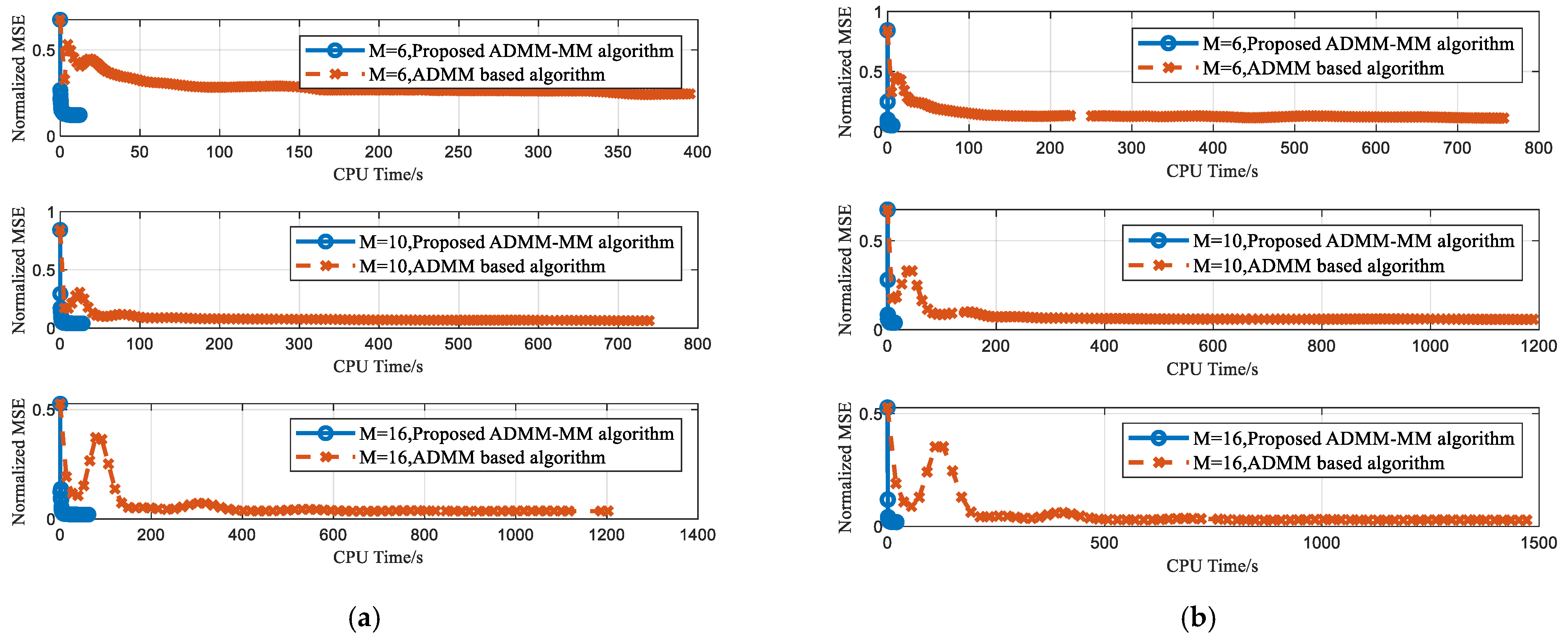
• Finally, the results of extensive simulation experiments demonstrate that the proposed algorithm outperforms the ADMM-based method [40] and exhibits superior computational efficiency. This validates the effectiveness and superiority of the proposed algorithm.

The rest of the paper is organized as follows. The system model is illustrated in Section 2. In Section 3, the proposed ADMM-MM algorithm is specified. Section 4 describes the simulation results and discussion, and a brief summary is presented in Section 5.

Notations: Boldface upper-case and lower-case letters denote matrices and column vectors, respectively. The scalars are denoted by italic letters. $x_i$ represents the $i$-th element of the vector $x$, and $X_{i,j}$ denotes the ($i$-th, $j$-th) element of the matrix $X$. $ℝ$ and $ℂ$ represent the real and complex fields. $\succcurlyeq$ represents the generalized inequality between matrices. $\left|\right|$, ${\Vert \cdot \Vert }_2$ and ${\Vert \cdot \Vert }_{\mathrm{F}}$ denote the absolution operation, Euclidean norm, and Frobenius norm, respectively. $\arg (\cdot )$ denotes the phase part of a complex number. The superscripts ${(\cdot )}^{*}$, ${(\cdot )}^{\mathrm{T}}$, and ${(\cdot )}^{\mathrm{H}}$ denote the complex conjugate, transpose, and conjugate transpose, respectively. $\mathrm{Tr}\left(X\right)$ denotes that the trace of $X$. $\mathrm{vec}\left(X\right)$ is a column vector consisting of all the columns of the matrix $X$ stacked. ${\lambda }_{\max }\left(X\right)$ represents the maximum eigenvalue of the matrix $X$. $\mathrm{Re}\left(x\right)$ and $\mathrm{Im}\left(x\right)$, respectively, represent the element-wise real part and image part of $x$. $I_N$ denotes an $N\times N$ identity matrix, and $\otimes$ denotes the Kronecker product.

2. System Model and Problem Formulation

As shown in Figure 1, we consider a collocated monostatic narrowband DFRC system based on a MIMO platform, which is equipped with $M$ antennas and arranged in the form of uniform linear arrays (ULAs), with half-wavelength spacing between the array elements. The DFRC system transmits radar-probing waveform $X\in {ℂ}^{M\times N}$ for $L$ point-like target detection, where $N$ is the number of snapshots in a radar pulse. We discretize the radar spatial detection region into $K$ parts and define ${\theta }_k$ as the $k$-th spatial angle. In addition, the transmit waveform can simultaneously serve $Q$ single antenna users on the downlink communication operation. In the following subsections, we provide a detailed description of the signal model and the formulation of the optimization problem.

2.1. Radar Model

The far-field-generated signal at the direction of ${\theta }_k$ can be written as $a_k{}^{\mathrm{H}}X$, and the power of the far-field-generated signal at ${\theta }_k$ is defined as

$$P_k=\frac{a_k{}^{\mathrm{H}}X{X}^{\mathrm{H}}{a}_k}{N}$$

(1)

where $a_k={\left[1,{\mathrm{e}}^{-j\pi \sin {\theta }_k},\dots ,{\mathrm{e}}^{-j\pi \left(M-1\right)\sin {\theta }_k}\right]}^{\mathrm{T}}$. Moreover, for the convenience of subsequent derivation and calculation, defining $x=\mathrm{vec}\left(X\right)$ and $A_k=I_N\otimes \left(a_k{a}_k{}^{\mathrm{H}}/N\right)$, $P_k$ can be rewritten as

$$P_k=x^{\mathrm{H}}{A}_{k}x$$

(2)

To enhance the radar detection performance of the DFRC system, it is necessary to focus energy on the target area, while suppressing the energy level in the sidelobe area and preventing the target echo from being obscured by noise. To achieve this, we minimize the MSE of beampattern matching as the cost function, which is defined as

$$f_{MSE}\left(x,\alpha \right)=\frac{1}{K}{\displaystyle \sum _{k=1}^K{\left|P_k-\alpha d_k\right|}^2}$$

(3)

where $\alpha$ is a scaling factor optimized jointly with $x$, and $d_k$ is the desired beampattern at ${\theta }_k$.

It is noteworthy that the coded waveform is usually used to design high-range and Doppler-resolution waveforms for moving target detection [41]. Thus, in addition to the MSE of beampattern matching, range and Doppler are also of interest for radar. However, if we take the MSE, range, and Doppler all into account for the designs of the DFRC system, the formulated problem will be extremely complicated and far beyond the scope of this paper. Thus, herein we only focus on the MSE of beampattern matching for radar.

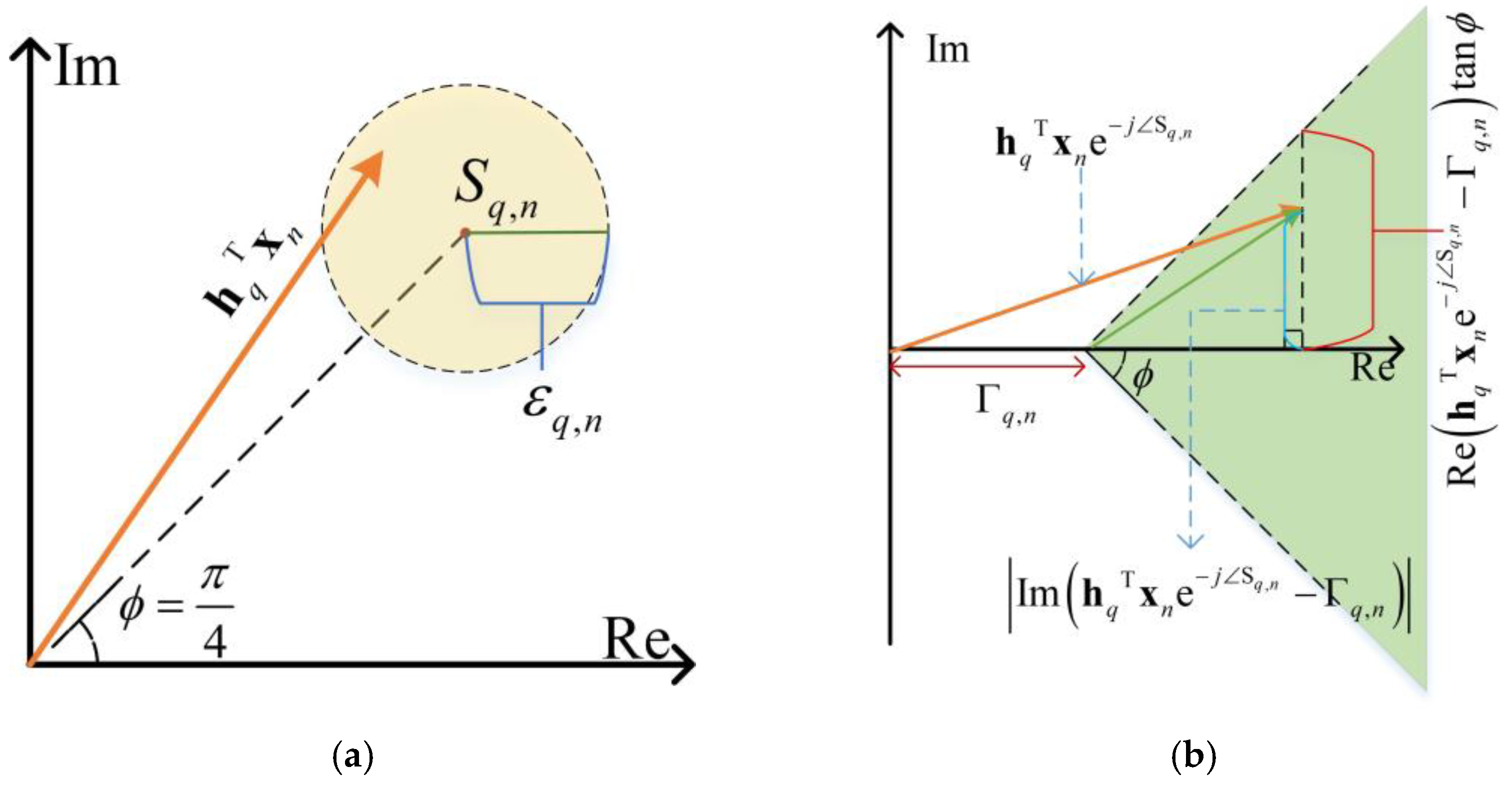
2.2. Communication QoS Constraints

In addition to its radar detection function, the DFRC system also simultaneously delivers information symbols to $Q$ single-antenna users using the same transmit waveform. The signals received by $Q$ users are given by

$$Y=HX+Z$$

(4)

where $H=\left[h_1{}^{\mathrm{T}};h_2{}^{\mathrm{T}};\dots ;h_Q{}^{\mathrm{T}}\right]\in {ℂ}^{Q\times M}$ is the channel matrix, and $h_q\in {ℂ}^{M\times 1}$ is the communication channel vector between the transmit array and the $q$-th communication user, $q=1,2,\dots ,Q$. $Z\in {ℂ}^{Q\times N}$ is the noise matrix in the $Q$ communication receivers.

To ensure the communication QoS of the DFRC system, two communication constraints are developed in the existing research: the MUI energy constraint and the CI constraint.

MUI energy constraint: According to [31,32,33,34], the received SINR per block of $N$ symbols for the $q$-th communication user is defined as

$${\mathrm{SINR}}_{q,c}=\frac{\mathbb{E}\left\{{\left|S_{q,n}\right|}^2\right\}}{\mathbb{E}\left\{{\left|h_q{}^{\mathrm{T}}{x}_n-S_{q,n}\right|}^2\right\}+N_0}$$

(5)

where $x_n$ is the $n$-th column of $X$, $N_0$ is the noise energy, $S_{q,n}$ is the desired communication signal, and $\mathbb{E}$ denotes the ensemble average with respect to the time index. The achievable sum rate of the communication part can be further expressed as

$${\mathrm{{\rm Y}}}_C={\displaystyle \sum _{q=1}^Q{\log }_2\left(1+{\mathrm{SIN}\mathrm{R}}_{q,c}\right)}$$

(6)

Clearly, the MUI energy directly affects the achievable sum rate of the downlink users. In order to obtain ${\mathrm{{\rm Y}}}_C$ that satisfies the communication requirements, the MUI energy must be brought below a predetermined threshold, which can be written as

$${\Vert HX-S\Vert }_F^2\le {\epsilon }^2$$

(7)

where $S$ is the desired constellation.

However, (7) is the traditional MUI energy constraint, which only constrains the total MUI energy. This does not guarantee the communication performance of each user at each time index. In this paper, as depicted in Figure 2a, we propose a more stringent per-user MUI energy constraint at each sampling moment as

$${\left|h_q{}^{\mathrm{T}}{x}_n-S_{q,n}\right|}^2\le {\epsilon }_{q,n}{}^2$$

(8)

Obviously, compared to the traditional MUI energy constraint, the proposed new constraint enables precise control over the performance of each transmitted communication signal. This has major practical significance and is worthy of further research. The corresponding achievable sum rate can be derived as

$${\mathrm{{\rm Y}}}_C\ge {\displaystyle \sum _{q=1}^Q{\log }_2\left(1+\frac{\mathbb{E}\left\{{\left|S_{q,n}\right|}^2\right\}}{{\displaystyle {\sum }_{n=1}^N{\epsilon }_{q,n}{}^2}/N+N_0}\right)}$$

(9)

Defining $i_n\in {ℂ}^{1\times N}$ is the $n$-th row of $I_N$ and taking an open root for (8), we can rewrite (8) as

$$\left|{\tilde{h}}_{q,n}{}^{\mathrm{T}}x-S_{q,n}\right|\le {\epsilon }_{q,n}$$

(10)

where ${\tilde{h}}_{q,n}{}^{\mathrm{T}}=i_n\otimes h_q{}^{\mathrm{T}}$.

CI constraint: In CI constraints, we do not consider all MUI energy to be harmful, and constructive interference can push the received signal toward the correct decision region, providing extra degrees of freedom for waveform design.

The CI technique has been extensively studied in recent research [35,36,37,38]. To avoid distracting from our main focus, we will not delve into the derivation of the CI constraint. Using the geometric relations for the rotated QPSK symbol illustrated in Figure 2b, the CI constraint can be easily formulated as

$$\mathrm{Re}\left(h_q{}^{\mathrm{T}}{x}_n{\mathrm{e}}^{-j\angle {\mathrm{S}}_{q,n}}\right)\tan \varphi -\left|\mathrm{Im}\left(h_q{}^{\mathrm{T}}{x}_n{\mathrm{e}}^{-j\angle {\mathrm{S}}_{q,n}}\right)\right|\ge {\mathrm{\Gamma }}_{q,n}\tan \varphi$$

(11)

where $\varphi =\pi /4$, ${\mathrm{\Gamma }}_{q,n}$ represents the minimum amplitude of the received noise-free signal. Assuming that $\zeta$ is the preset signal-to-noise ratio (SNR) threshold of communication users and ${\delta }_{q,n}{}^2$ is the power of noise, we can obtain ${\left|h_q{}^{\mathrm{T}}{x}_n\right|}^2/{\delta }_{q,n}{}^2\ge \zeta$. Then, ${\mathrm{\Gamma }}_{q,n}$ can be derived as

$${\mathrm{\Gamma }}_{q,n}=\left|h_q{}^{\mathrm{T}}{x}_n\right|\ge {\delta }_{q,n}\sqrt{\zeta }.$$

(12)

Furthermore, defining

$${\overline{h}}_{2q,n}{}^{\mathrm{T}}\triangleq \left(i_n\otimes h_q{}^{\mathrm{T}}\right){\mathrm{e}}^{-j\angle {\mathrm{S}}_{qn}}\left(\tan \varphi -{\mathrm{e}}^{-j\frac{\pi }{2}}\right)$$

(13)

$${\overline{h}}_{2q-1,n}{}^{\mathrm{T}}\triangleq \left(i_n\otimes h_q{}^{\mathrm{T}}\right){\mathrm{e}}^{-j\angle {\mathrm{S}}_{qn}}\left(\tan \varphi +{\mathrm{e}}^{-j\frac{\pi }{2}}\right)$$

(14)

finally, we can rewrite (12) as

$$\mathrm{Re}\left({\overline{h}}_{i,n}{}^{\mathrm{T}}x\right)\ge {\overline{\mathrm{\Gamma }}}_{i,n}\tan \varphi$$

(15)

where ${\overline{\mathrm{\Gamma }}}_{i,n}=\{\begin{array}{l}\begin{array}{cc}{\mathrm{\Gamma }}_{q,n}& i=2q\end{array}\\ \begin{array}{cc}{\mathrm{\Gamma }}_{q,n}& i=2q-1\end{array}\end{array}$, $i=1,2,\dots ,2Q$, $n=1,2,\dots ,N$.

Remark 1.

(1) The downlink channel $H$ experiences flat Rayleigh fading but remains constant within a single communication frame or radar pulse. (2) The channel $H$ is assumed to be perfectly estimated at the DFRC system via a training-based method.

2.3. Problem Formulation

Based on the above discussion, we aim in this paper to design an integrated transmit waveform to minimize the radar beampattern mismatch while satisfying the predefined communication QoS constraints. Additionally, we add a constant modulus constraint to ensure that the transmit waveform has an unimodular property, maximizing the efficiency of the radio frequency (RF) amplifier and preventing nonlinear distortions. Finally, according to different QoS constraints in communication, we can formulate two optimization problems, as shown below:

$${𝒫}_1\{\begin{array}{ll}\underset{x,\alpha }{\min }& f_{MSE}\left(x,\alpha \right)\hfill \\ \mathrm{s}.\mathrm{t}.& \left|{\tilde{h}}_{q,n}{}^{\mathrm{T}}x-S_{q,n}\right|\le {\epsilon }_{q,n}\hfill \\ & \forall q=1,2,\dots ,Q;n=1,2,\dots ,N\hfill \\ & \left|x\left(j\right)\right|=1\hspace{1em}\forall j=1,2,\dots ,MN\hfill \end{array}$$

(16)

$${𝒫}_2\{\begin{array}{ll}\underset{x,\alpha }{\min }& f_{MSE}\left(x,\alpha \right)\hfill \\ \mathrm{s}.\mathrm{t}.& \mathrm{Re}\left({\overline{h}}_{i,n}{}^{\mathrm{T}}x\right)\ge {\overline{\mathrm{\Gamma }}}_{i,n}\tan \varphi \\ & \forall i=1,2,\dots ,2Q;n=1,2,\dots ,N\hfill \\ & \left|x\left(j\right)\right|=1\begin{array}{c}\end{array}\forall j=1,2,\dots ,MN\hfill \end{array}.$$

Both ${𝒫}_1$ and ${𝒫}_2$ exhibit non-convex characteristics due to their intricate multivariate challenges and stringent equation constraints. Fortunately, these issues can be addressed using the ADMM-based algorithm proposed in [40,42]. However, the proposed ADMM-based algorithm necessitates the utilization of off-the-shelf algorithms and optimization tools (such as the interior point method and CVX toolbox) to solve the subproblem, resulting in high computational complexity at each iteration. As the number of array elements and downlink communication users increases, the computational complexity becomes impractical.

To reconcile this contradiction, this article proposes a novel ADMM-MM algorithm to tackle these problems more efficiently. Further elaborations on the specifics of this algorithm can be found in the subsequent section.

3. Proposed Algorithm

As both ${𝒫}_1$ and ${𝒫}_2$ involve multiple variables, we first simplify them into two more manageable univariate problems. By fixing the value of $x$, both ${𝒫}_1$ and ${𝒫}_2$ can be transformed into the same form as

$$\begin{array}{cc}\underset{\alpha }{\min }& f_{MSE}\left(\alpha \right)=\frac{1}{K}{\displaystyle \sum _{k=1}^K{\left|x^{\mathrm{H}}{A}_{k}x-\alpha d_k\right|}^2}\end{array}.$$

(17)

Equation (17) represents an unconstrained differentiable problem, and its optimal solution can be obtained by setting the derivative to 0. Thus, the optimal $\alpha$ can be derived as

$${\alpha }_{opt}=\frac{{\displaystyle \sum _{k=1}^K{d}_k{x}^{\mathrm{H}}{A}_{k}x}}{{\displaystyle \sum _{k=1}^K{d}_k{}^2}}.$$

(18)

By substituting (18) into $f_{MSE}\left(x,\alpha \right)$, the cost function of ${𝒫}_1$ and ${𝒫}_2$ can be simplified into a univariate function:

$$f_{MSE}\left(x\right)=\frac{1}{K}{\displaystyle \sum _{k=1}^K{\left|x^{\mathrm{H}}{B}_{k}x\right|}^2}$$

(19a)

where

$$B_k=A_k-d_k\frac{{\displaystyle \sum _{k=1}^K{d}_k{A}_k}}{{\displaystyle \sum _{k=1}^K{d}_k{}^2}}.$$

(19b)

3.1. Proposed ADMM-MM Algorithm for Solving ${𝒫}_1$

As described in the previous section, ${𝒫}_1$ can be rewritten as

$${𝒫}_1\{\begin{array}{cc}\underset{x}{\min }& \frac{1}{K}{\displaystyle {\sum }_{k=1}^K{\left|x^{\mathrm{H}}{B}_{k}x\right|}^2}\hfill \\ \mathrm{s}.\mathrm{t}.& \left|{\tilde{h}}_{q,n}{}^{\mathrm{T}}x-S_{q,n}\right|\le {\epsilon }_{q,n}\hfill \\ & \forall q=1,2,\dots ,Q;n=1,2,\dots ,N\hfill \\ & \left|x\left(j\right)\right|=1\begin{array}{c}\end{array}\forall j=1,2,\dots ,MN\hfill \end{array}$$

(20)

Firstly, we transform the MUI energy constraint into a simple form. Defining

$${{\rm T}}_1\left(k_1,:\right)={\tilde{h}}_{q,n}{}^{\mathrm{T}}$$

(21a)

$${\mathsf{\Psi }}_1\left(k_1\right)={\epsilon }_{q,n}$$

(21b)

where ${{\rm T}}_1\left(k_1,:\right)$ denotes $k_1$-th row of ${{\rm T}}_1\in {ℂ}^{QN\times MN}$, ${\mathsf{\Psi }}_1\left(k_1\right)$ denotes $k_1$-th element of ${\Psi }_1\in {ℂ}^{QN\times 1}$, and $k_1=\left(n-1\right)\times Q+q$.

${𝒫}_1$ can be further rewritten as

$${𝒫}_1\{\begin{array}{ll}\underset{x}{\min }& \frac{1}{K}{\displaystyle {\sum }_{k=1}^K{\left|x^{\mathrm{H}}{B}_{k}x\right|}^2}\\ \mathrm{s}.\mathrm{t}.& \mathrm{abs}\left(T_{1}x-s\right)\le {\Psi }_1\\ & \left|x\left(j\right)\right|=1\begin{array}{c}\end{array}\forall j=1,2,\dots ,MN\hfill \end{array}$$

(22)

where $s=\mathrm{vec}\left(S\right)$ and $\mathrm{abs}(\cdot )$ denotes an element-wise absolution operation.

Defining

$$y=T_{1}x-s$$

(23a)

$$\mathbb{I}\left(x\right)=\{\begin{array}{cc}0\hfill & \hfill \left|x\left(j\right)\right|=1\\ +\infty \hfill & \hfill otherwise\end{array}$$

(23b)

$$\mathbb{I}\left(y\right)=\{\begin{array}{cc}0\hfill & \hfill \mathrm{abs}\left(y\right)\le {\Psi }_1\\ +\infty \hfill & \hfill otherwise\end{array}$$

(23c)

${𝒫}_1$ can be derived as

$${{𝒫}^{\prime }}_1\{\begin{array}{ll}\underset{x,y}{\min }& \frac{1}{K}{\displaystyle \sum _{k=1}^K{\left|x^{\mathrm{H}}{B}_{k}x\right|}^2+\mathbb{I}\left(x\right)+\mathbb{I}\left(y\right)}\hfill \\ \mathrm{s}.\mathrm{t}.& y=T_{1}x-s\hfill \end{array}$$

(24)

We can solve ${{𝒫}_1}^{\prime }$ by tackling its augmented Lagrangian function, which can be written as

$$ℒ\left(x,y,u\right)=\frac{1}{K}{\displaystyle \sum _{k=1}^K{\left|x^{\mathrm{H}}{B}_{k}x\right|}^2}+\mathbb{I}\left(x\right)+\mathbb{I}\left(y\right)+\frac{{\rho }_1}{2}{\Vert y-T_{1}x+s+u/{\rho }_1\Vert }_2^2$$

(25)

where ${\rho }_1$ is the penalty parameter, and $u$ is the dual variable corresponding to $y=T_{1}x-s$. Clearly, in the $\left(l+1\right)$-th iteration, the ADMM framework consists of the following procedures:

$$x^{\left(l+1\right)}=\begin{array}{cc}\underset{x}{\arg \min }& ℒ\end{array}\left(x,y^{\left(l\right)},u^{\left(l\right)}\right)$$

(26a)

$$y^{\left(l+1\right)}=\begin{array}{cc}\underset{y}{\arg \min }& ℒ\left(x^{\left(l+1\right)},y,u^{\left(l\right)}\right)\end{array}$$

(26b)

$$u^{\left(l+1\right)}=u^{\left(l\right)}+{\rho }_1\left(y^{\left(l+1\right)}-T_1{x}^{\left(l+1\right)}+s\right).$$

(26c)

Next, we further derive the solutions of (26a) and (26b) to update $x^{\left(l+1\right)}$ and $y^{\left(l+1\right)}$.

3.1.1. Solution to (26a)

Problem (26a) can be rewritten as

$$\begin{array}{cc}\underset{x}{\min }& \frac{1}{K}{\displaystyle \sum _{k=1}^K{\left|x^{\mathrm{H}}{B}_{k}x\right|}^2}+\mathbb{I}\left(x\right)+\mathbb{I}\left(y^{\left(l\right)}\right)+\frac{{\rho }_1}{2}{\Vert y^{\left(l\right)}-T_{1}x+s+u^{\left(l\right)}/{\rho }_1\Vert }_2^2\end{array}.$$

(27)

By removing extraneous constant terms, we obtain

$${𝒫}_{1ℒ\left(x\right)}\{\begin{array}{ll}\underset{x}{\min }& \frac{1}{K}{\displaystyle \sum _{k=1}^K{\left|x^{\mathrm{H}}{B}_{k}x\right|}^2}+\frac{{\rho }_1}{2}{\Vert y^{\left(l\right)}-T_{1}x+s+u^{\left(l\right)}/{\rho }_1\Vert }_2^2\\ \mathrm{s}.\mathrm{t}.& \left|x\left(i\right)\right|=1\begin{array}{c}\end{array}\forall i=1,2,\dots ,MN\end{array}.$$

(28)

Defining $t^{\left(l\right)}=y^{\left(l\right)}+u^{\left(l\right)}/{\rho }_1+s$, ${𝒫}_{1ℒ\left(x\right)}$ can be derived as

$${𝒫}_{1ℒ\left(x\right)}\{\begin{array}{ll}\underset{x}{\min }& \frac{1}{K}{\displaystyle \sum _{k=1}^K{\left|x^{\mathrm{H}}{B}_{k}x\right|}^2}+\frac{{\rho }_1}{2}{x}^{\mathrm{H}}{T}_1{}^{\mathrm{H}}{T}_{1}x-{\rho }_1\mathrm{Re}\left(x^{\mathrm{H}}{T}_1{}^{\mathrm{H}}{t}^{\left(l\right)}\right)\\ \mathrm{s}.\mathrm{t}.& \left|x\left(i\right)\right|=1\hspace{1em}\forall i=1,2,\dots ,MN\end{array}$$

(29)

We use the MM algorithm to solve ${𝒫}_{1ℒ(x)}$. Firstly, we look for the upper bound function of $\frac{1}{K}{\displaystyle \sum _{k=1}^K{\left|x^{\mathrm{H}}{B}_{k}x\right|}^2}$ and $\frac{{\rho }_1}{2}{x}^{\mathrm{H}}{T}_1{}^{\mathrm{H}}{T}_{1}x$, respectively. Defining $\overline{x}=x{x}^{\mathrm{H}}$, $\frac{1}{K}{\displaystyle \sum _{k=1}^K{\left|x^{\mathrm{H}}{B}_{k}x\right|}^2}$ can be rewritten as

$$\frac{1}{K}{\displaystyle \sum _{k=1}^K{\left|x^{\mathrm{H}}{B}_{k}x\right|}^2}={\mathrm{vec}}^{\mathrm{H}}\left(\overline{x}\right)C\mathrm{vec}\left(\overline{x}\right)$$

(30a)

where

$$C=\frac{1}{K}{\displaystyle \sum _{k=1}^K\mathrm{vec}\left(B_k\right){\mathrm{vec}}^{\mathrm{H}}\left(B_k\right)}$$

(30b)

In the following, we introduce a useful lemma as follows.

Lemma 1.

The quadratic form $x^{\mathrm{H}}Lx$, where $L$ is a Hermitian matrix, can be upper-bounded as

$$x^{\mathrm{H}}Lx\le x^{\mathrm{H}}Mx+2\mathrm{Re}\left[x^{\mathrm{H}}\left(L-M\right)x^{\left(l\right)}\right]+{\left(x^{\left(l\right)}\right)}^{\mathrm{H}}\left(M-L\right)x^{\left(l\right)}$$

(31)

where  $M\succcurlyeq L$, $x^{\left(l\right)}$  is the value of  $x$  at the  $l$-th iteration.

Applying Lemma 1, we can derive

$$\begin{array}{l}{\mathrm{vec}}^{\mathrm{H}}\left(\overline{x}\right)C\mathrm{vec}\left(\overline{x}\right)\\ \le {\lambda }_{\max }\left(C\right){\mathrm{vec}}^{\mathrm{H}}\left(\overline{x}\right)\mathrm{vec}\left(\overline{x}\right)+2\mathrm{Re}\left[{\mathrm{vec}}^{\mathrm{H}}\left(\overline{x}\right)\left(C-{\lambda }_{\max }\left(C\right)I_{M^2{N}^2}\right)\mathrm{vec}\left({\overline{x}}^{\left(l\right)}\right)\right]\\ +{\mathrm{vec}}^{\mathrm{H}}\left({\overline{x}}^{\left(l\right)}\right)\left({\lambda }_{\max }\left(C\right)I_{M^2{N}^2}-C\right)\mathrm{vec}\left({\overline{x}}^{\left(l\right)}\right)\end{array}$$

(32)

where ${\lambda }_{\max }\left(C\right)$ denotes the maximum eigenvalue of $C$. Due to the high dimensions of $C$, calculating its maximum eigenvalue produces significant computational complexity. However, the special structure of $C$ enables us to conduct dimensionality reduction, which can effectively reduce the computational burden. The specific derivation details are provided in the Appendix A.

The third term on the right-hand side of (32) is constant and can be disregarded. Additionally, the first term in (32) can be simplified to a constant term $M^2{N}^2{\lambda }_{\max }\left(C\right)$. As a result, we can simplify (32) as

$${\mathrm{vec}}^{\mathrm{H}}\left(\overline{x}\right)C\mathrm{vec}\left(\overline{x}\right)\le x^{\mathrm{H}}Dx+const$$

(33a)

where $const$ denotes constant term, and

$$D=D_1-2{\lambda }_{\max }\left(C\right)x^{\left(l\right)}{\left(x^{\left(l\right)}\right)}^{\mathrm{H}}$$

(33b)

$$D_1=\frac{2}{K}{\displaystyle \sum _{k=1}^K{\left(x^{\left(l\right)}\right)}^{\mathrm{H}}{B}_k{x}^{\left(l\right)}{B}_k}$$

(33c)

Continuing the application of Lemma 1, due to ${\lambda }_{\max }\left(D_1\right)I_{MN}\succcurlyeq D_1\succcurlyeq D$, we can obtain

$$x^{\mathrm{H}}Dx\le \mathrm{Re}\left(x^{\mathrm{H}}{b}_1\right)+const$$

(34a)

where

$$b_1=2\left(D{x}^{\left(l\right)}-{\lambda }_{\max }\left(D_1\right)x^{\left(l\right)}\right)$$

(34b)

Due to $B_k\preccurlyeq A_k$, ${\lambda }_{\max }\left(D_1\right)$ can be calculated as

$$\begin{array}{ll}{\lambda }_{\max }\left(D_1\right)& \le \frac{2}{K}{\displaystyle \sum _{k=1}^K\left[{\left(x^{\left(l\right)}\right)}^{\mathrm{H}}{B}_k{x}^{\left(l\right)}{\lambda }_{\max }\left(B_k\right)\right]}\\ & \le \frac{2}{K}{\displaystyle \sum _{k=1}^K\left[{\left(x^{\left(l\right)}\right)}^{\mathrm{H}}{B}_k{x}^{\left(l\right)}{\lambda }_{\max }\left(A_k\right)\right]}\\ & \le \frac{2M}{KN}{\displaystyle \sum _{k=1}^K\left[{\left(x^{\left(l\right)}\right)}^{\mathrm{H}}{B}_k{x}^{\left(l\right)}\right]}\end{array}$$

(35)

The upper bound function of $\frac{{\rho }_1}{2}{x}^{\mathrm{H}}{T}_1{}^{\mathrm{H}}{T}_{1}x$ can be obtained by

$$\frac{{\rho }_1}{2}{x}^{\mathrm{H}}{T}_1{}^{\mathrm{H}}{T}_{1}x\le \mathrm{Re}\left(x^{\mathrm{H}}{b}_2\right)+const$$

(36a)

where

$$b_2={\rho }_1\left[T_1{}^{\mathrm{H}}{T}_1{x}^{\left(l\right)}-{\lambda }_{\max }\left(T_1{}^{\mathrm{H}}{T}_1\right)x^{\left(l\right)}\right]$$

(36b)

Thus, the majorized problem of ${𝒫}_{1ℒ\left(x\right)}$ can be formulated as

$$\begin{array}{ll}\underset{x}{\max }& \mathrm{Re}\left(x^{\mathrm{H}}\left(-U_1\right)\right)\\ \mathrm{s}.\mathrm{t}.& \left|x\left(j\right)\right|=1\hspace{1em}\forall j=1,2,\dots ,MN\end{array}$$

(37)

where $U_1=b_1+b_2-{\rho }_1{T}_1{}^{\mathrm{H}}{t}^{\left(l\right)}$, and it is easy to verify that the solution to (37) is given by

$$x^{\left(l+1\right)}{=\mathrm{e}}^{j\arg \left(-U_1\right)}$$

(38)

where $\arg (\cdot )$ denotes an element-wise phase extraction operation.

3.1.2. Solution to (26b)

Problem (26b) can be written as

$${𝒫}_{1ℒ\left(y\right)}\{\begin{array}{ll}\underset{y}{\min }& {\Vert y-p^{\left(l\right)}\Vert }_2^2\\ \mathrm{s}.\mathrm{t}.& \mathrm{abs}\left(y\right)\le {\Psi }_1\end{array}$$

(39a)

where

$$p^{\left(l\right)}=T_1{x}^{\left(l+1\right)}-s-u^{\left(l\right)}/{\rho }_1$$

(39b)

We can solve ${𝒫}_{1ℒ\left(y\right)}$ by translating it into the elemental level. Assuming $y_i$, $p_i^{\left(l\right)}$ and ${\Psi }_1\left(i\right)$ are, respectively, the $i$-th element of the vector $y$, $p^{\left(l\right)}$ and ${\Psi }_1$, (39a) can be updated as follows:

$$\begin{array}{cc}\underset{y_i}{\min }& \left|y_i-p_i^{\left(l\right)}\right|\\ s.\mathrm{t}.& \left|y_i\right|\le {\Psi }_1\left(i\right)\end{array}$$

(40)

It can be verified that the solution to (40) is

$$y_i=\{\begin{array}{cc}\hspace{1em}{p}_i^{\left(l\right)},& \left|p_i^{\left(l\right)}\right|\le {\Psi }_1\left(i\right)\\ \frac{p_i^{\left(l\right)}}{\left|p_i^{\left(l\right)}\right|}{\Psi }_1\left(i\right),& \left|p_i^{\left(l\right)}\right|>{\Psi }_1\left(i\right)\end{array}$$

(41)

Finally, we summarize the proposed ADMM-MM algorithm for solving ${𝒫}_1$ in Algorithm 1, and the termination criteria can be defined as

$${\Vert d_{r1}{}^{\left(l+1\right)}\Vert }_2={\Vert y^{\left(l+1\right)}-T_1{x}^{\left(l+1\right)}+s\Vert }_2\ge {\mathrm{\Delta }}_{r1}{}^{\left(l+1\right)}$$

(42a)

$${\Vert d_{s1}{}^{\left(l+1\right)}\Vert }_2={\Vert {\rho }_1\left(y^{\left(l+1\right)}-y^{\left(l\right)}\right)\Vert }_2\ge {\mathrm{\Delta }}_{s1}{}^{\left(l+1\right)}$$

(42b)

where $d_{r1}{}^{\left(l+1\right)}$ and $d_{s1}{}^{\left(l+1\right)}$ are the primal residual and dual residual at $l+1$ iteration. The feasibility tolerances for the primal and dual feasibility conditions are denoted by ${\mathrm{\Delta }}_{r1}{}^{\left(l+1\right)}$ and ${\mathrm{\Delta }}_{s1}{}^{\left(l+1\right)}$, respectively. These tolerances can be adjusted based on accuracy requirements, and specific parameter settings details can be found in [42].

Algorithm 1: Proposed ADMM-MM algorithm for solving ${𝒫}_1$
Input: ${\rho }_1$, $K$, $M$, $N$, $Q$, $A_k$, $B_k$, $T_1$, ${\Psi }_1$, $s$. Output: $x_{opt}$
1	Initialize: l = 0, $x^{\left(l\right)}$, $y^{\left(l\right)}$, $u^{\left(l\right)}$.
	Repeat
		// Update  $x^{\left(l+1\right)}$
2		Calculate ${\lambda }_{\max }\left(C\right)$ and ${\lambda }_{\max }\left(D_1\right)$ according to Appendix A and Equation (35).
3		Derive $b_1$ according to Equation (34b).
4		Derive $b_2$ according to Equation (36b).
5		Compute $x^{\left(l+1\right)}$ by solving Equation (38).
		// Update  $y^{\left(l+1\right)}$  and  $u^{\left(l+1\right)}$
6		Compute $y^{\left(l+1\right)}$ by solving Equation (41).
7		Compute $u^{\left(l+1\right)}$ by solving Equation (26c).
8		l = l + 1.
	Until the termination criteria (42) are met
9	$x_{opt}=x^{(l)}$

3.2. Proposed ADMM-MM Algorithm for ${𝒫}_2$

Firstly, we rewrite the CI constraint of ${𝒫}_2$ as

$$\mathrm{Re}\left({{\rm T}}_{2}x\right)\ge {\Psi }_2$$

(43)

where ${{\rm T}}_2\left(k_2,:\right)={\overline{h}}_{i,n}{}^{\mathrm{T}}$, ${\mathsf{\Psi }}_2\left(k_2\right)={\overline{\mathrm{\Gamma }}}_{i,n}\tan \varphi$, and $k_2=\left(n-1\right)\times 2Q+i$.

Similar to the previous Section 3.1, introducing an auxiliary variable $\gamma$, the augmented Lagrangian function of ${𝒫}_2$ can be derived as

$$ℒ\left(x,\gamma ,\upsilon \right)=\frac{1}{K}{\displaystyle \sum _{k=1}^K{\left|x^{\mathrm{H}}{B}_k{}^{\mathrm{H}}x\right|}^2}+\mathbb{I}\left(x\right)+\mathbb{I}\left(\gamma \right)+\frac{{\rho }_2}{2}{\Vert \gamma -{{\rm T}}_{2}x+\upsilon /{\rho }_2\Vert }_2^2$$

(44a)

$$\mathbb{I}(\gamma )=\{\begin{array}{cc}0\hfill & \mathrm{Re}\left(\gamma \right)\ge {\Psi }_2\\ +\infty & otherwise\end{array}$$

(44b)

where ${\rho }_2$ is the penalty parameter and $\upsilon$ is the dual variable. Next, in the $\left(l+1\right)$-th iteration, we separately update $x^{\left(l+1\right)}$, ${\gamma }^{\left(l+1\right)}$ and ${\upsilon }^{\left(l+1\right)}$ as

$$x^{\left(l+1\right)}=\begin{array}{cc}\underset{x}{\arg \min }& ℒ\end{array}\left(x,{\gamma }^{\left(l\right)},{\upsilon }^{\left(l\right)}\right)$$

(45a)

$${\gamma }^{\left(l+1\right)}=\begin{array}{cc}\underset{\gamma }{\arg \min }& ℒ\left(x^{\left(l+1\right)},\gamma ,{\upsilon }^{\left(l\right)}\right)\end{array}$$

(45b)

$${\upsilon }^{\left(l+1\right)}={\upsilon }^{\left(l\right)}+{\rho }_2\left({\gamma }^{\left(l+1\right)}-T_2{x}^{\left(l+1\right)}\right).$$

(45c)

3.2.1. Solution to (45a)

We can update $x^{\left(l+1\right)}$ by solving

$${𝒫}_{2ℒ\left(x\right)}\{\begin{array}{ll}\underset{x}{\min }& \frac{1}{K}{\displaystyle \sum _{k=1}^K{\left|x^{\mathrm{H}}{B}_k{}^{\mathrm{H}}x\right|}^2}+\frac{{\rho }_2}{2}{\Vert {{\rm T}}_{2}x-\left({\upsilon }^{\left(l\right)}/{\rho }_2+{\gamma }^{\left(l\right)}\right)\Vert }_2^2\\ \mathrm{s}.\mathrm{t}.& \left|x\left(i\right)\right|=1\hspace{1em}\forall i=1,2,\dots ,MN\end{array}.$$

(46)

Applying Lemma 1, we can obtain the upper bound function of ${𝒫}_{2ℒ\left(x\right)}$ as

$$\begin{array}{l}\frac{1}{K}{\displaystyle \sum _{k=1}^K{\left|x^{\mathrm{H}}{B}_k{}^{\mathrm{H}}x\right|}^2}+\frac{{\rho }_2}{2}{\Vert {{\rm T}}_{2}x-\left({\upsilon }^{\left(l\right)}/{\rho }_2+{\gamma }^{\left(l\right)}\right)\Vert }_2^2\\ \le \mathrm{Re}\left(x^{\mathrm{H}}{b}_1\right)+\frac{{\rho }_2}{2}{x}^{\mathrm{H}}{{\rm T}}_2{}^{\mathrm{H}}{{\rm T}}_{2}x-{\rho }_2\mathrm{Re}\left[x^{\mathrm{H}}{{\rm T}}_2{}^{\mathrm{H}}\left({\upsilon }^{\left(l\right)}/{\rho }_2+{\gamma }^{\left(l\right)}\right)\right]+const\\ \le \mathrm{Re}\left\{x^{\mathrm{H}}\left[b_1+b_3-{{\rm T}}_2{}^{\mathrm{H}}\left({\upsilon }^{\left(l\right)}+{\rho }_2{\gamma }^{\left(l\right)}\right)\right]\right\}+const\end{array}$$

(47a)

where

$$b_3={\rho }_2\left[{{\rm T}}_2{}^{\mathrm{H}}{{\rm T}}_2{x}^{\left(l\right)}-{\lambda }_{\max }\left({{\rm T}}_2{}^{\mathrm{H}}{{\rm T}}_2\right)x^{\left(l\right)}\right].$$

(47b)

Thus, the majorized problem of ${𝒫}_{2ℒ\left(x\right)}$ can be formulated as

$$\begin{array}{ll}\underset{x}{\max }& \mathrm{Re}\left(x^{\mathrm{H}}\left(-U_2\right)\right)\\ \mathrm{s}.\mathrm{t}.& \left|x\left(j\right)\right|=1\begin{array}{c}\end{array}\forall j=1,2,\dots ,MN\end{array}$$

(48)

where $U_2=b_1+b_3-{{\rm T}}_2{}^{\mathrm{H}}\left({\upsilon }^{\left(l\right)}+{\rho }_2{\gamma }^{\left(l\right)}\right)$, and the solution to (48) can be given as

$$x^{\left(l+1\right)}{=\mathrm{e}}^{j\arg \left(-U_2\right)}$$

(49)

3.2.2. Solution to (45b)

We can update ${\gamma }^{\left(l+1\right)}$ by solving

$${𝒫}_{2ℒ\left(\gamma \right)}\{\begin{array}{l}\begin{array}{cc}\underset{\gamma }{\min }& {\Vert \gamma -{\zeta }^{\left(l\right)}\Vert }_2^2\end{array}\\ \begin{array}{cc}\mathrm{s}.\mathrm{t}.& \begin{array}{c}\end{array}\mathrm{Re}\left(\gamma \right)\ge {\Psi }_2\end{array}\end{array}$$

(50a)

where

$${\zeta }^{\left(l\right)}={{\rm T}}_2{x}^{\left(l+1\right)}-\frac{{\upsilon }^{\left(l\right)}}{{\rho }_2}$$

(50b)

Similar to the previous Section 3.1.2, it can be verified that the solution to (50a) is

$$\mathrm{Re}\left({\gamma }_i\right)=\{\begin{array}{cc}\mathrm{Re}\left({\zeta }_i^{\left(l\right)}\right),& \mathrm{Re}\left({\zeta }_i^{\left(l\right)}\right)\ge {\Psi }_2\left(i\right)\\ {\Psi }_2\left(i\right),\hfill & \mathrm{Re}\left({\zeta }_i^{\left(l\right)}\right)<{\Psi }_2\left(i\right)\end{array}$$

(51a)

$$\mathrm{Im}\left({\gamma }_i\right)=\mathrm{Im}\left({\zeta }_i^{\left(l\right)}\right)$$

(51b)

$${\gamma }_i=\mathrm{Re}\left({\gamma }_i\right)+j\mathrm{Im}\left({\gamma }_i\right)$$

(51c)

where ${\gamma }_i$ is the $i$-th element of $\gamma$, ${\zeta }_i^{\left(l\right)}$ and ${\Psi }_2\left(i\right)$ are, respectively, the $i$-th element of ${\zeta }^{\left(l\right)}$ and ${\Psi }_2$. Finally, the proposed ADMM-MM algorithm for solving ${𝒫}_2$ is summarized in Algorithm 2, and the termination criteria are defined as

$${\Vert d_{r2}{}^{\left(l+1\right)}\Vert }_2={\Vert {\gamma }^{\left(l+1\right)}-{{\rm T}}_2{x}^{\left(l+1\right)}\Vert }_2\ge {\mathrm{\Delta }}_{r2}{}^{\left(l+1\right)}$$

(52a)

$${\Vert d_{s2}{}^{\left(l+1\right)}\Vert }_2={\Vert {\rho }_2\left({\gamma }^{\left(l+1\right)}-{\gamma }^{\left(l\right)}\right)\Vert }_2\ge {\mathrm{\Delta }}_{s2}{}^{\left(l+1\right)}.$$

(52b)

Algorithm 2: Proposed ADMM-MM algorithm for solving ${𝒫}_2$
Input: ${\rho }_2$, $K$, $M$, $N$, $Q$, $A_k$, $B_k$, ${{\rm T}}_2$, ${\Psi }_2$, $s$. Output: $x_{opt}$
1	Initialize: l = 0, $x^{\left(l\right)}$, ${\gamma }^{\left(l\right)}$, ${\upsilon }^{\left(l\right)}$.
	Repeat
		// Update $x^{\left(l+1\right)}$
2		Derive $b_1$ according to Equation (34b).
3		Derive $b_3$ according to Equation (47b).
4		Compute $x^{\left(l+1\right)}$ by solving Equation (49).
		// Update ${\gamma }^{(l+1)}$ and ${\upsilon }^{\left(l+1\right)}$
5		Compute ${\gamma }^{\left(l+1\right)}$ by solving Equation (51).
6		Compute ${\upsilon }^{\left(l+1\right)}$ by solving Equation (45c).
7		l = l + 1.
	Until the termination criteria (52) are met
8	$x_{opt}=x^{(l)}$

3.3. Computational Complexity Analysis

The computational complexities of both Algorithms 1 and 2 are determined on the basis of the number of iterations and the complexity of each iteration. To provide a better understanding, we summarize the corresponding computational complexities at each iteration for both algorithms in

Table 1. Computational Complexity for Solving ${𝒫}_1$.

Computation		Complexity
Update $x$	${\lambda }_{\max }(C)$	$O(M^6)$
	${\lambda }_{\max }(D_1)$	$O(KMN)$
	${\lambda }_{\max }({{\rm T}}_1{}^{\mathrm{H}}{{\rm T}}_1)$	$O(M^3{N}^3)$
	$b_1$	$O(M^3{N}^3)$
	$b_2$	$O(Q{M}^2{N}^3)$
Update $y$		$O(QM{N}^2)$
Update $u$		$O(QM{N}^2)$
Total	$O(M^6+M^3{N}^3+Q{M}^2{N}^3+QM{N}^2+KMN)$

and

Table 2. Computational Complexity for Solving ${𝒫}_2$.

Computation		Complexity
Update $x$	${\lambda }_{\max }(C)$	$O(M^6)$
	${\lambda }_{\max }(D_1)$	$O(KMN)$
	${\lambda }_{\max }({{\rm T}}_2{}^{\mathrm{H}}{{\rm T}}_2)$	$O(M^3{N}^3)$
	$b_1$	$O(M^3{N}^3)$
	$b_3$	$O(2Q{M}^2{N}^3)$
Update $\gamma$		$O(2QM{N}^2)$
Update $\upsilon$		$O(2QM{N}^2)$
Total	$O(M^6+M^3{N}^3+2Q{M}^2{N}^3+2QM{N}^2+KMN)$

.

4. Results

In this section, we provide several numerical examples to demonstrate the performance of the proposed algorithm. Unless stated otherwise, the following simulation parameters are used throughout this section. We set the number of transmit antennas as $M=10$, and collect $N=32$ samples in one pulse interval. We assume that the spatial area of interest is $\left[-{90}^{°},{90}^{°}\right]$, and the total number of spatial angle discretions is $K=181$. For radar function, according to the DFRC system settings in [42], we assume that the desired beampattern of the DFRC system possesses three principal lobes, located at $\left[-{50}^{°},-{30}^{°}\right]\cup \left[-{10}^{°},{10}^{°}\right]\cup \left[{30}^{°},{50}^{°}\right]$. For downlink communication, we predefine the number of communication users as $Q=2$. Without a loss of generality, we consider the estimated channel $h_q$ to be a complex Gaussian distribution, satisfying $h_q\sim \mathcal{C}\mathcal{N}(0,1/MN)$. The desired symbol matrix $S$ is generated according to the unit power QPSK alphabet. The communication QoS is separately assumed as ${\epsilon }_{q,n}={10}^{-1}$ and ${\mathrm{\Gamma }}_{q,n}=1$, $\forall q$, $\forall n$.

We performed all the analyses on an ordinary computer with an Intel Core i7-10750H CPU and 16 GB of RAM.

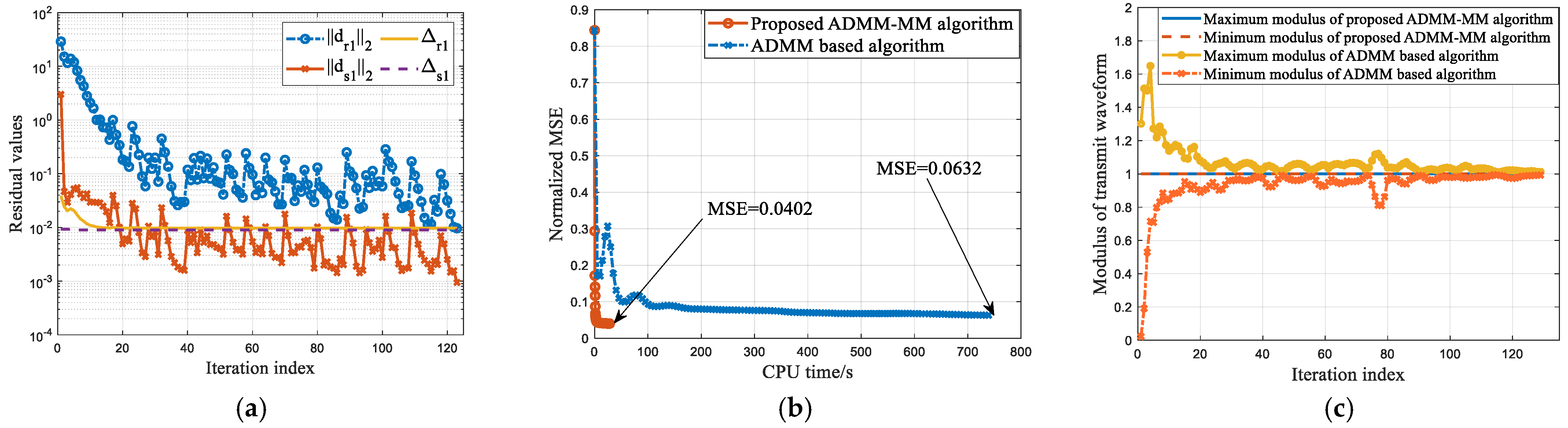
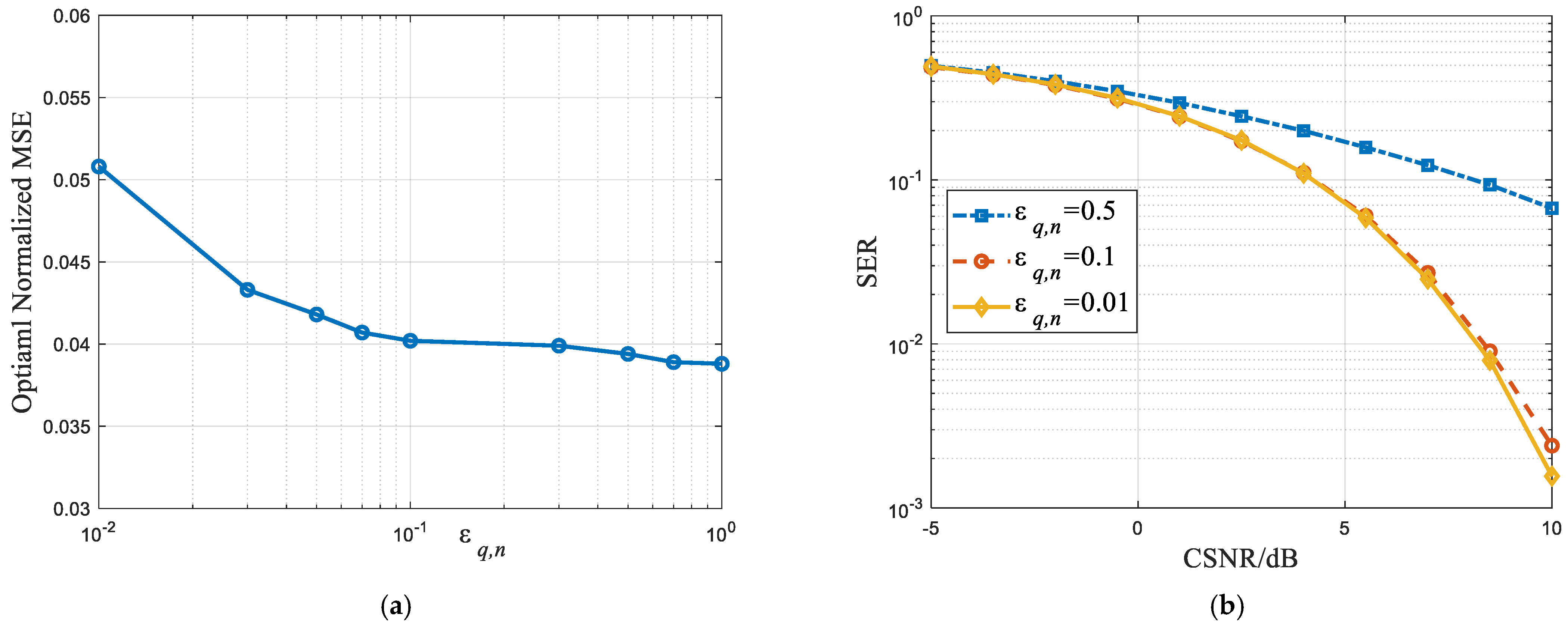
4.1. Effective Analysis of the Proposed Algorithm for Solving ${𝒫}_1$

In Figure 3, we first analyze the convergence performance of the proposed ADMM-MM algorithm in terms of its capacity to solve ${𝒫}_1$. Figure 3a illustrates the convergence of primal and dual residuals. It is evident that the proposed ADMM-MM algorithm successfully satisfies termination conditions after approximately 100 iterations, thus demonstrating its ability to converge within a finite number of iterations. To showcase the superiority of the proposed method, we conduct a convergence comparison with the existing ADMM-based approach [40] in Figure 3b. It is readily apparent that the proposed algorithm achieves a lower normalized MSE in terms of radar beampattern matching and exhibits faster convergence, requiring less CPU time compared to the ADMM based method [40]. Furthermore, Figure 3c presents the modulus of the transmit waveform as a function of the number of iterations. Notably, due to the utilization of the MM framework, the proposed ADMM-MM algorithm consistently maintains a constant waveform modulus during convergence, aligning more closely with the original problem.

The normalized received beampatterns of the radar which are required to solve ${𝒫}_1$ are depicted in Figure 4a. It is evident that the use of radar alone offers better beampattern performance. Compared to the only-radar technique, the proposed method suffers a little performance loss due to the communication constraint. However, we find that the proposed method provides a closer approximation to the desired beampattern and lower sidelobe level compared to the ADMM based method [40], resulting in better detection performance. In Figure 4b, the noiseless signals received by communication users are illustrated. It is evident that both the proposed ADMM-MM algorithm and the ADMM based method in [40] successfully satisfy the MUI energy constraints of the per-user noiseless signal received at each sampling moment.

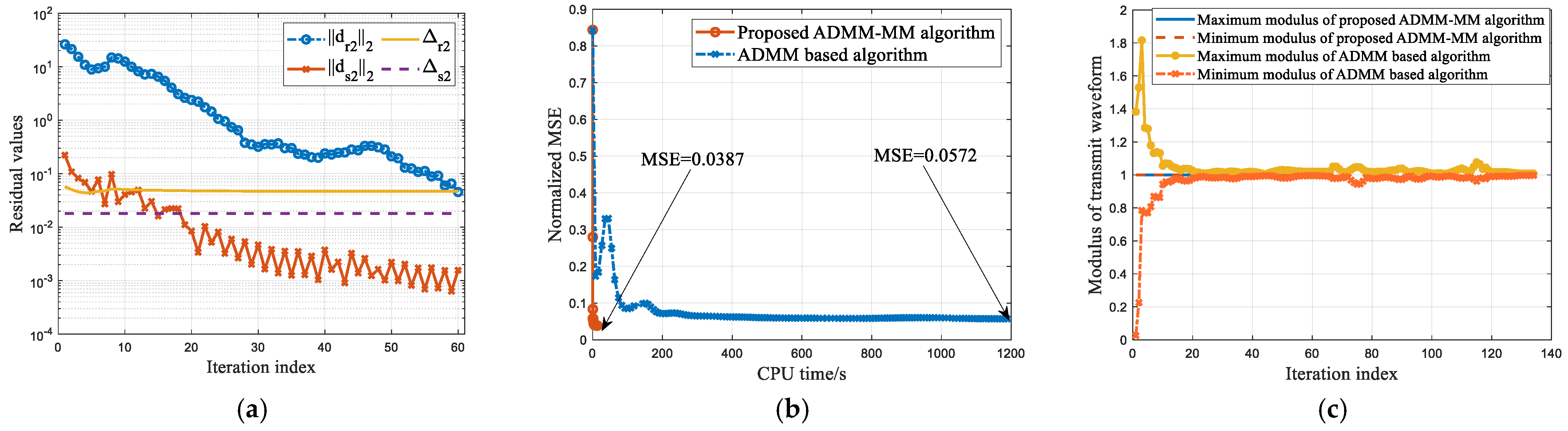
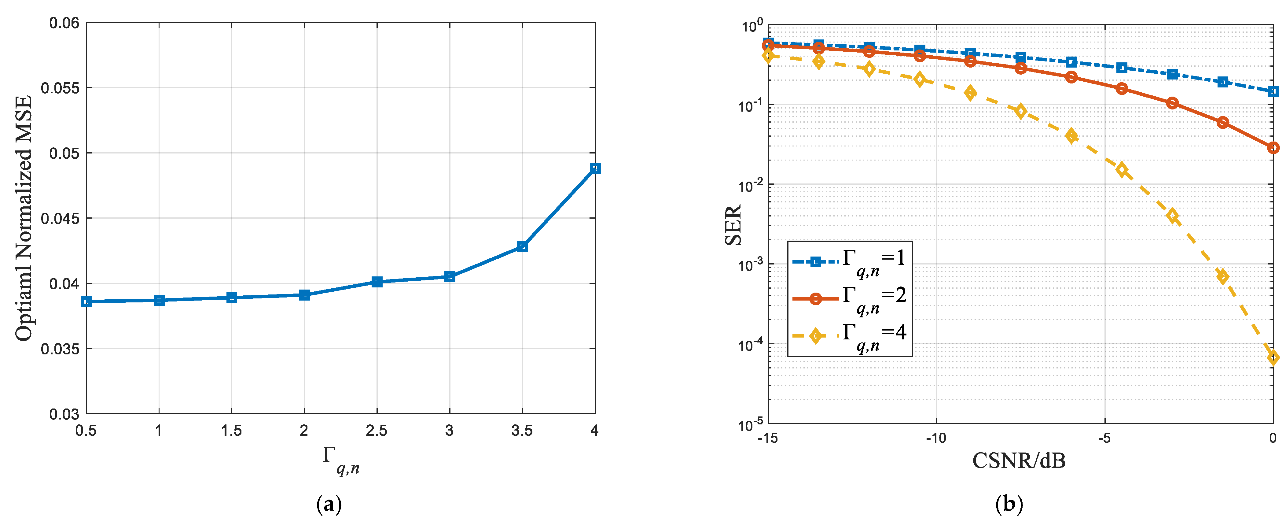
4.2. Effective Analysis of the Proposed Algorithm for Solving ${𝒫}_2$

As in the previous Section 4.1, we analyze the effectiveness of the proposed method for solving ${𝒫}_2$. The convergence performance of the proposed ADMM-MM algorithm when solving ${𝒫}_2$ is depicted in Figure 5. It is evident that the proposed algorithm successfully satisfies termination conditions after dozens of iterations, requiring fewer iterations and less CPU time to converge than the ADMM based method [40]. Additionally, it is readily observable that the proposed algorithm achieves a lower normalized MSE of the radar beampattern matching and consistently maintains a constant waveform modulus during convergence.

Figure 6a depicts the normalized received beampattern of the radar for solving ${𝒫}_2$. It is evident that the proposed method can obtain a very similar beampattern with only radar. Additionally, the proposed method exhibits lower sidelobe levels and superior beampattern matching performance compared to the ADMM based method [40]. This outcome validates the superiority of the proposed method. Figure 6b illustrates the noiseless signals received by communication users. It is evident that both the proposed ADMM-MM algorithm and the ADMM based method in [40] effectively ensure that the noiseless received signals reside within the CI region, thereby satisfying the communication CI constraints of ${𝒫}_2$.

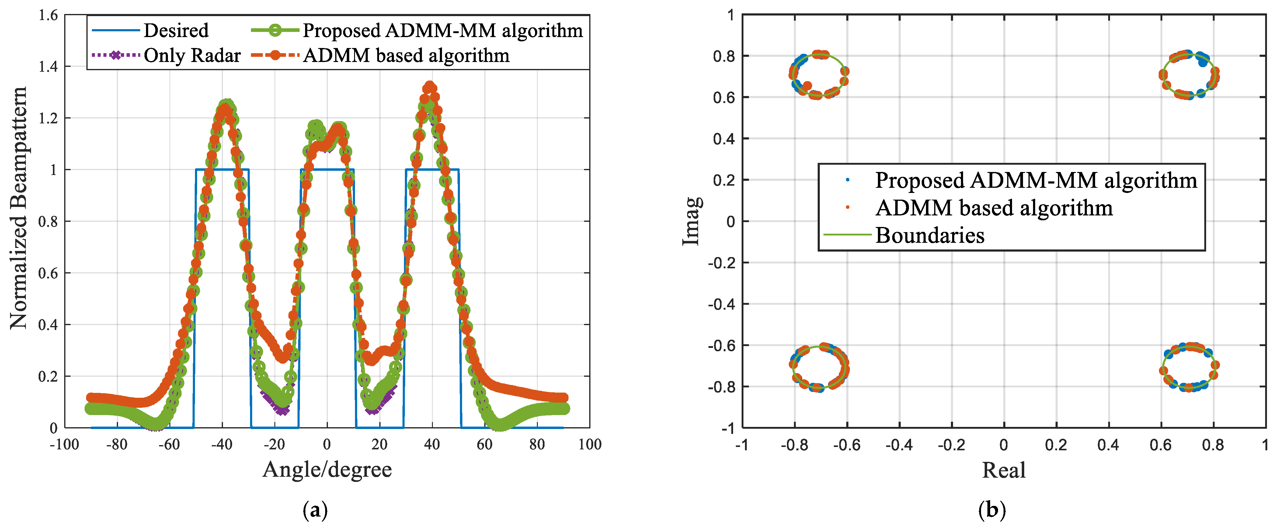
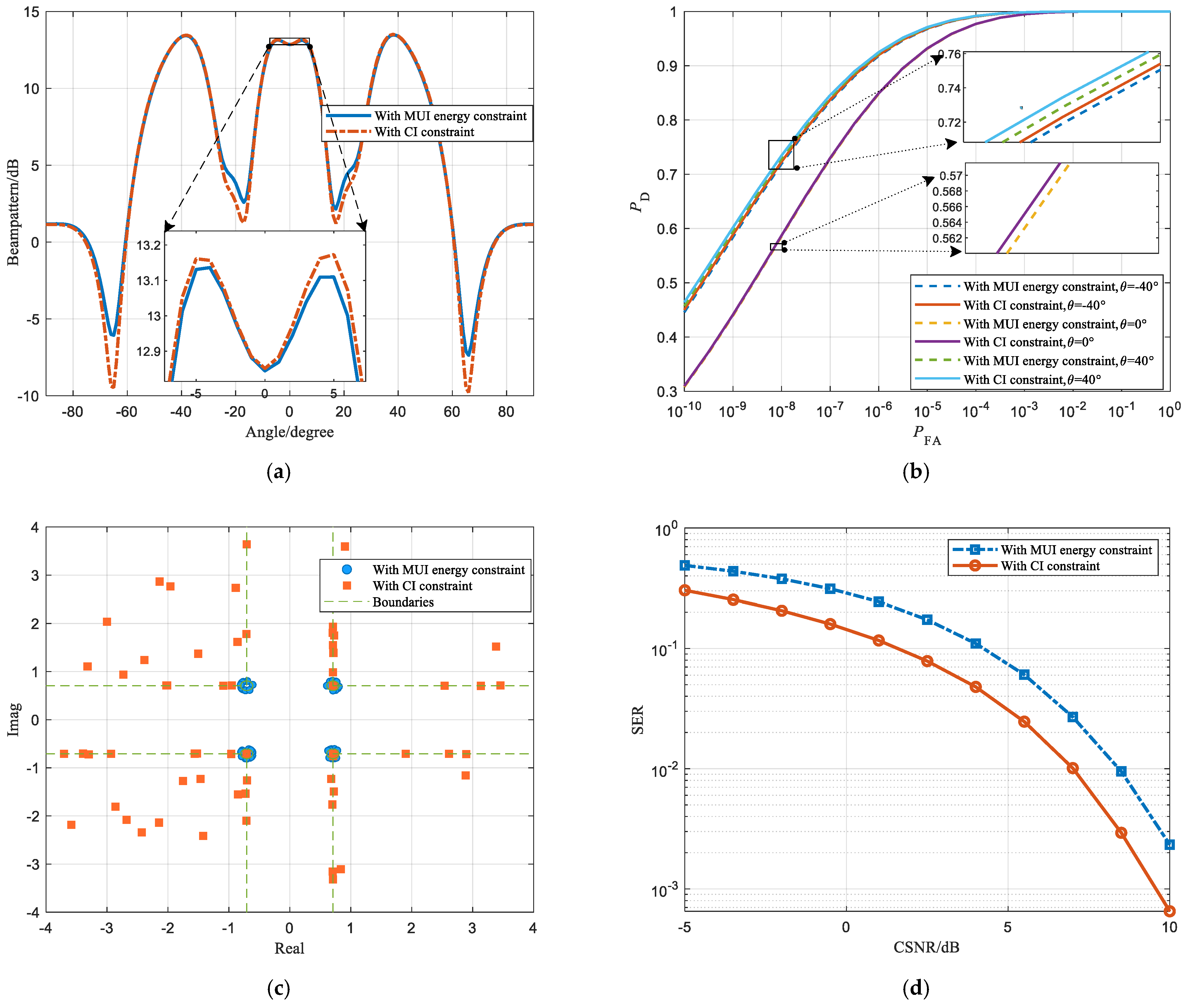
4.3. Performance Analysis

Here, we outline how communication QoS affects DFRC system performance. Figure 7 illustrates the optimal normalized MSE and SER of the DFRC system as a function of the communication MUI energy ${\epsilon }_{q,n}$ when solving ${𝒫}_1$. It is expected to observe a decrease in the normalized MSE of beampattern matching as the MUI energy constraint ${\epsilon }_{q,n}$ increases. This trade-off between radar sensing and wireless communication performance is a well-documented limitation of the DFRC system. Furthermore, it is evident that a smaller MUI energy results in a lower BER, thereby leading to improved communication performance. Figure 8 depicts the optimal normalized MSE and SER of the DFRC system versus the communication QoS requirements ${\mathrm{\Gamma }}_{q,n}$ when solving ${𝒫}_2$. It is evident that the normalized MSE increases as ${\mathrm{\Gamma }}_{q,n}$ rises, indicating a decline in radar detection performance with higher communication QoS.

Next, we present a performance comparison between ${𝒫}_1$ and ${𝒫}_2$. It is worth noting that the desired communication constellation energy remains consistent for both the MUI energy constraint and CI constraint, and ${\mathrm{\Gamma }}_{q,n}=1$, ${\epsilon }_{q,n}={10}^{-1}$.

Figure 9a illustrates the performance comparison of the radar component. It is evident that ${𝒫}_1$ and ${𝒫}_2$ exhibit similar beampatterns, with ${𝒫}_2$ demonstrating a higher mainlobe level and lower sidelobe level. This distinction arises from the CI constraint being more relaxed than the MUI energy constraint, leading to a larger feasibility region and enhanced radar performance. To further evaluate the target detection performance, we present the receiver operating characteristic (ROC) by plotting the detection probability $P_{\mathrm{D}}$ versus the false alarm probability $P_{\mathrm{FA}}$ in Figure 9b. It can be observed that, with the same false alarm probability, e.g., ${10}^{-8}$, ${𝒫}_2$ can achieve higher detection probability than ${𝒫}_1$, illustrating the superiority of CI constraint for radar detection.

The performance comparison of the communication component is presented in Figure 9c,d. Figure 9c draws the received communication constellations, showing that the synthesized communication signals in ${𝒫}_2$ are more sparsely distributed and have higher power, intuitively suggesting a better communication performance than ${𝒫}_1$. To further validate this assertion, we provide the symbol error rate (SER) analysis in Figure 9d, where the results of ${10}^4$ independent trials are displayed. It is evident that the SER decreases as the communication signal-to-noise ratio (CSNR) increases for both ${𝒫}_1$ and ${𝒫}_2$. However, when the CSNR is fixed, ${𝒫}_2$ achieves a lower SER compared to ${𝒫}_1$, illustrating the superiority of CI constraints for communication.

Finally, we can conclude that the CI constraint is more relaxed compared to the MUI constraint, which is advantageous for obtaining better optimization results and achieving superior radar performance. Additionally, the CI constraint usually enables a higher communication signal power than the MUI energy constraint, and this extra power is beneficial for communication decoding. Thus, in comparison to the MUI constraint, we believe that the CI constraint is more suitable for addressing the integrated waveform design problem of the DFRC system.

4.4. Computational Efficiency Comparison with the ADMM based Method in [40]

Next, we will proceed to compare the computational efficiency of the proposed method and the ADMM based method [40] at different system scales.

Figure 10 draws the normalized MSE curves versus CPU time for various cohort sizes of communicating users ($Q$ = 2, 3, and 4). It can be observed that, whether with MUI constraint or CI constraint, an increase in the number of communication users results in more stringent communication constraints for the DFRC system, leading to a smaller feasibility region, larger normalized MSE, and a degradation in radar performance. Moreover, a larger $Q$ requires more CPU time to attain the local optimal solution due to the increased complexity caused by the smaller feasibility region and larger system scale.

Subsequently, we investigate the influence of the number of antennas on the performance of the DFRC system. The normalized MSE curves versus CPU time for different numbers of antennas ($M$ = 6, 10, and 16) are shown in Figure 11. It is evident that, whether solving ${𝒫}_1$ or ${𝒫}_2$, the addition of antennas leads to improved radar detection performance in different methods. This enhancement arises from increased waveform diversity and the ability of the DFRC system to obtain higher beamforming gains. However, a larger number of antennas results in a larger system scale, leading to slower convergence.

Furthermore, the convergence comparison between the proposed ADMM-MM method and the ADMM-based method [40] is shown in

Table 3. Convergence comparison between the proposed ADMM-MM method and the ADMM based method [40].

		Proposed ADMM-MM Method	ADMM based Method [40]
		MSE/Runtime (s)	MSE/Runtime (s)
Solving ${𝒫}_1$	$Q=2$, $M=6$	0.1220/12.21	0.2450/395.06
	$Q=2$, $M=10$	0.0402/28.09	0.0632/738.74
	$Q=2$, $M=16$	0.0200/61.84	0.0362/1202.51
	$Q=3$, $M=10$	0.0578/40.20	0.1208/956.67
	$Q=4$, $M=10$	0.0724/120.10	0.1794/3063.91
Solving ${𝒫}_2$	$Q=2$, $M=6$	0.0519/5.95	0.1121/756.49
	$Q=2$, $M=10$	0.0387/13.15	0.0572/1189.18
	$Q=2$, $M=16$	0.0191/20.39	0.0278/1741.21
	$Q=3$, $M=10$	0.0394/21.93	0.0637/1801.28
	$Q=4$, $M=10$	0.0397/25.72	0.0718/3261.77

. It is important to emphasize that for any given $Q$ or $M$, our proposed ADMM-MM method can obtain better optimization results and achieve faster convergence compared to the ADMM-based methods [40]. This is because the approach in reference [40] combines multiple optimization variables into a higher-dimensional variable, resulting in a complex problem solution space that hinders the identification of the optimal solution. Moreover, the use of off-the-shelf algorithms and optimization tools, such as the interior point method and CVX toolbox, in [40] introduces considerable computational complexity during each iteration of solving the subproblem. In contrast, our proposed method effectively uses the strong coupling relationship between $\alpha$ and waveform $x$, and we additionally employ the MM algorithm and exploit the geometric structure to address the subproblems. As a result, our method demonstrates superior performance and significantly improved efficiency.

5. Conclusions

In this paper, we investigated two waveform design problems for the DFRC system, considering different constrained communication QoS requirements. The normalized MSE of radar beampattern matching was minimized as a cost function while formulating stricter per-user MUI energy constraints at each sampling moment and CI constraint, respectively. We added a constant modulus constraint to preserve the unimodular property of the transmit waveform. To tackle the complicated non-convex problems, we proposed a novel ADMM-MM algorithm. Finally, simulation results demonstrated that the proposed algorithm outperforms the ADMM-based algorithm [40] and exhibits superior computational efficiency. This validated the effectiveness and superiority of the proposed algorithm. However, the proposed ADMM-MM algorithm still requires careful selection of appropriate penalty parameters and cannot fully address the issue of waveform design for the DFRC system when channel estimation is inaccurate. Therefore, building upon our current work, we are motivated to further investigate robust waveform design for the DFRC system in the presence of uncertain channel estimation.

References

1. Ali, A.; Zhu, Y.; Zakarya, M. Exploiting dynamic spatio-temporal correlations for citywide traffic flow prediction using attention based neural networks. Inf. Sci. 2021, 577, 852–870. [Google Scholar] [CrossRef]
2. Ali, A.; Zhu, Y.; Zakarya, M. A data aggregation based approach to exploit dynamic spatio-temporal correlations for citywide crowd flows prediction in fog computing. Multimed. Tools Appl. 2021, 80, 31401–31433. [Google Scholar] [CrossRef]
3. Ali, A.; Zhu, Y.; Zakarya, M. Exploiting dynamic spatio-temporal graph convolutional neural networks for citywide traffic flows prediction. Neural Netw. 2022, 145, 233–247. [Google Scholar] [CrossRef] [PubMed]
4. Aubry, A.; Carotenuto, V.; De Maio, A.; Farina, A.; Pallotta, L. Optimization theory-based radar waveform design for spectrally dense environments. IEEE Aerosp. Electron. Syst. Mag. 2016, 31, 14–25. [Google Scholar] [CrossRef]
5. Guo, B.; Liang, J.; Wang, G.; Tang, B.; So, H.C. Bistatic MIMO DFRC System Waveform Design via Fractional Programming. IEEE Trans. Signal Process. 2023, 71, 1952–1967. [Google Scholar] [CrossRef]
6. Liu, F.; Masouros, C.; Petropulu, A.P.; Griffiths, H.; Hanzo, L. Joint radar and communication design: Applications, state-of-the-art, and the road ahead. IEEE Trans. Commun. 2020, 68, 3834–3862. [Google Scholar] [CrossRef]
7. Zhao, Y.; Zhao, Z.; Tong, F.; Sun, P.; Feng, X.; Zhao, Z. Joint Design of Transmitting Waveform and Receiving Filter via Novel Riemannian Idea for DFRC System. Remote Sens. 2023, 15, 3548. [Google Scholar] [CrossRef]
8. Huang, C.; Huang, Z.; Zhou, Q.; Zhang, J.; Yang, Z.; Zhang, K. Unimodular waveform design for integrated radar communication and jamming. Digit. Signal Process. 2023, 143. [Google Scholar] [CrossRef]
9. Yang, R.; Jiang, H.; Qu, L. Waveform Design for MIMO Dual-Functional Radar-Communication System Using MUI Energy Minimization With PAPR and CRB Constraints. IEEE Commun. Lett. 2023, 27, 1417–1421. [Google Scholar] [CrossRef]
10. Li, H.; Liu, Y.; Liao, G.; Chen, Y. Joint Radar and Communications Waveform Design Based on Complementary Sequence Sets. Remote Sens. 2023, 15, 645. [Google Scholar] [CrossRef]
11. Zhang, J.A.; Liu, F.; Masouros, C.; Heath, R.W.; Feng, Z.; Zheng, L.; Petropulu, A. An overview of signal processing techniques for joint communication and radar sensing. IEEE J. Sel. Top. Signal Process. 2021, 15, 1295–1315. [Google Scholar] [CrossRef]
12. Euziere, J.; Guinvarc’h, R.; Lesturgie, M.; Uguen, B.; Gillard, R. Dual Function Radar Communication Time-Modulated Array. In Proceedings of the 2014 International Radar Conference, Lille, France, 13–17 October 2014; pp. 1–4. [Google Scholar]
13. Hassanien, A.; Amin, M.G.; Zhang, Y.D.; Ahmad, F. Dual-function radar-communications: Information embedding using sidelobe control and waveform diversity. IEEE Trans. Signal Process. 2015, 64, 2168–2181. [Google Scholar] [CrossRef]
14. BouDaher, E.; Hassanien, A.; Aboutanios, E.; Amin, M.G. Towards a Dual-Function MIMO Radar-Communication System. In Proceedings of the 2016 IEEE Radar Conference (RadarConf), Philadelphia, PA, USA, 2–6 May 2016; pp. 1–6. [Google Scholar]
15. Hassanien, A.; Amin, M.G.; Zhang, Y.D.; Ahmad, F. Signaling strategies for dual-function radar communications: An overview. IEEE Aerosp. Electron. Syst. Mag. 2016, 31, 36–45. [Google Scholar] [CrossRef]
16. Hassanien, A.; Amin, M.G.; Zhang, Y.D.; Ahmad, F. Phase-modulation based dual-function radar-communications. IET Radar Sonar Navig. 2016, 10, 1411–1421. [Google Scholar] [CrossRef]
17. Ahmed, A.; Zhang, Y.D.; Gu, Y. Dual-function radar-communications using QAM-based sidelobe modulation. Digit. Signal Process. 2018, 82, 166–174. [Google Scholar] [CrossRef]
18. Wu, W.; Cao, Y.; Wang, S.; Yeo, T.; Wang, M. MIMO waveform design combined with constellation mapping for the integrated system of radar and communication. Signal Process. 2020, 170, 107443. [Google Scholar] [CrossRef]
19. Hassanien, A.; Aboutanios, E.; Amin, M.G.; Fabrizio, G.A. A dual-function MIMO radar-communication system via waveform permutation. Digit. Signal Process. 2018, 83, 118–128. [Google Scholar] [CrossRef]
20. Wang, X.; Hassanien, A.; Amin, M.G. Dual-function MIMO radar communications system design via sparse array optimization. IEEE Trans. Aerosp. Electron. Syst. 2018, 55, 1213–1226. [Google Scholar] [CrossRef]
21. Ma, D.; Shlezinger, N.; Huang, T.; Liu, Y.; Eldar, Y.C. FRaC: FMCW-based joint radar-communications system via index modulation. IEEE J. Sel. Top. Signal Process. 2021, 15, 1348–1364. [Google Scholar] [CrossRef]
22. Huang, T.; Shlezinger, N.; Xu, X.; Liu, Y.; Eldar, Y.C.J. MAJoRCom: A dual-function radar communication system using index modulation. IEEE Trans. Signal Process. 2020, 68, 3423–3438. [Google Scholar] [CrossRef]
23. Baxter, W.; Aboutanios, E.; Hassanien, A. Joint radar and communications for frequency-hopped MIMO systems. IEEE Trans. Signal Process. 2022, 70, 729–742. [Google Scholar] [CrossRef]
24. Xu, J.; Wang, X.; Aboutanios, E.; Cui, G. Hybrid index modulation for dual-functional radar communications systems. IEEE Trans. Veh. Technol. 2022, 72, 3186–3200. [Google Scholar] [CrossRef]
25. Wu, K.; Zhang, J.A.; Huang, X.; Guo, Y.J. Frequency-hopping MIMO radar-based communications: An overview. IEEE Aerosp. Electron. Syst. Mag. 2021, 37, 42–54. [Google Scholar] [CrossRef]
26. Liu, Y.; Liao, G.; Chen, Y.; Xu, J.; Yin, Y. Super-resolution range and velocity estimations with OFDM integrated radar and communications waveform. IEEE Trans. Veh. Technol. 2020, 69, 11659–11672. [Google Scholar] [CrossRef]
27. Liyanaarachchi, S.D.; Riihonen, T.; Barneto, C.B.; Valkama, M. Optimized waveforms for 5G–6G communication with sensing: Theory, simulations and experiments. IEEE Trans. Wirel. Commun. 2021, 20, 8301–8315. [Google Scholar] [CrossRef]
28. Liu, Y.; Liao, G.; Yang, Z. Robust OFDM integrated radar and communications waveform design based on information theory. Signal Process. 2019, 162, 317–329. [Google Scholar] [CrossRef]
29. Sit, Y.L.; Nuss, B.; Zwick, T. On mutual interference cancellation in a MIMO OFDM multiuser radar-communication network. IEEE Trans. Veh. Technol. 2018, 67, 3339–3348. [Google Scholar] [CrossRef]
30. Rong, J.; Liu, F.; Miao, Y. Integrated Radar and Communications Waveform Design Based on Multi-Symbol OFDM. Remote Sens. 2022, 14, 4705. [Google Scholar] [CrossRef]
31. Liu, F.; Zhou, L.; Masouros, C.; Li, A.; Luo, W.; Petropulu, A. Toward Dual-Functional Radar-Communication Systems: Optimal Waveform Design. IEEE Trans. Signal Process. 2018, 66, 4264–4279. [Google Scholar] [CrossRef]
32. Shi, S.; Wang, Z.; He, Z.; Cheng, Z. Constrained Waveform Design for Dual-Functional MIMO Radar-Communication System. Signal Process. 2020, 171, 107530. [Google Scholar] [CrossRef]
33. Huang, Z.; Tang, B.; Huang, C.; Qin, L. Direct Transmit Waveform Design to Match a Desired Beampattern under the Constant Modulus Constraint. Digit. Signal Process. 2022, 126, 103486. [Google Scholar] [CrossRef]
34. Jiang, M.; Liao, G.; Yang, Z.; Liu, Y.; Chen, Y. Integrated Radar and Communication Waveform Design Based on a Shared Array. Signal Process. 2021, 182, 107956. [Google Scholar] [CrossRef]
35. Wang, B.; Wu, L.; Cheng, Z.; He, Z. Exploiting Constructive Interference in Symbol Level Hybrid Beamforming for Dual-Function Radar-Communication System. IEEE Wirel. Commun. Lett. 2022, 11, 2071–2075. [Google Scholar] [CrossRef]
36. Zhang, Z.; Chang, Q.; Liu, F.; Yang, S. Dual-functional radar-communication waveform design: Interference reduction versus exploitation. IEEE Commun. Lett. 2021, 26, 148–152. [Google Scholar] [CrossRef]
37. Su, N.; Liu, F.; Wei, Z.; Liu, Y.-F.; Masouros, C. Secure dual-functional radar-communication transmission: Exploiting interference for resilience against target eavesdropping. IEEE Trans. Wirel. Commun. 2022, 21, 7238–7252. [Google Scholar] [CrossRef]
38. Liu, R.; Li, M.; Liu, Q.; Swindlehurst, A.L. Joint Waveform and Filter Designs for STAP-SLP-Based MIMO-DFRC Systems. IEEE J. Sel. Areas Commun. 2022, 40, 1918–1931. [Google Scholar] [CrossRef]
39. Liu, R.; Li, M.; Liu, Q.; Swindlehurst, A.L. Dual-Functional Radar-Communication Waveform Design: A Symbol-Level Precoding Approach. IEEE J. Sel. Top. Signal Process. 2021, 15, 1316–1331. [Google Scholar] [CrossRef]
40. Zhang, T.; Zhao, Y.; Liu, D.; Chen, J. Interference Optimized Dual-Functional Radar-Communication Waveform Design with Low PAPR and Range Sidelobe. Signal Process. 2023, 204, 108828. [Google Scholar] [CrossRef]
41. Zhu, J.; Song, Y.; Jiang, N.; Xie, Z.; Fan, C.; Huang, X. Enhanced Doppler Resolution and Sidelobe Suppression Performance for Golay Complementary Waveforms. Remote Sens. 2023, 15, 2452. [Google Scholar] [CrossRef]
42. Cheng, Z.; He, Z.; Zhang, S.; Li, J. Constant Modulus Waveform Design for MIMO Radar Transmit Beampattern. IEEE Trans. Signal Process. 2017, 65, 4912–4923. [Google Scholar] [CrossRef]
43. Horn, R.A.; Johnson, C.R. Matrix Analysis; Cambridge University Press: Cambridge, UK, 2012. [Google Scholar]
Figure 1. Illustration of a collocated narrowband DFRC system.
Remotesensing 15 05350 g001
Figure 2. Illustration of two communication QoS constraints. (a) Per-user per-time MUI energy constraint; (b) CI constraint.
Remotesensing 15 05350 g002
Figure 3. Convergence performance verification of the proposed algorithm for solving 𝒫 1 . (a) Residual curves versus the number of iterations; (b) normalized MSE versus CPU time, in comparison with ADMM based method [40]; (c) modulus of transmit waveform versus the number of iterations, in comparison with ADMM based method [40].
Remotesensing 15 05350 g003
Figure 4. (a) Normalized received beampatterns for solving 𝒫 1 , in comparison with only-radar and ADMM based method [40]; (b) received communication constellations for solving 𝒫 1 , in comparison with ADMM based method [40].
Remotesensing 15 05350 g004
Figure 5. Convergence performance verification of the proposed algorithm for solving 𝒫 2 . (a) Residual curves versus the number of iterations; (b) normalized MSE versus CPU time, in comparison with ADMM based method [40]; (c) modulus of transmit waveform versus the number of iterations, in comparison with ADMM based method [40].
Remotesensing 15 05350 g005
Figure 6. (a) Normalized received beampatterns for solving 𝒫 2 , in comparison with only-radar and ADMM based method [40]; (b) received communication constellations for solving 𝒫 2 , in comparison with ADMM based method [40].
Remotesensing 15 05350 g006
Figure 7. Performance analysis for different ε q , n . (a) Optimal normalized MSE versus ε q , n ; (b) SER versus CSNR for different ε q , n .
Remotesensing 15 05350 g007
Figure 8. Performance analysis for different Γ q , n . (a) Optimal normalized MSE versus Γ q , n ; (b) SER versus CSNR for different Γ q , n .
Remotesensing 15 05350 g008
Figure 9. Performance comparison between 𝒫 1 and 𝒫 2 . (a) Beampattern performance; (b) P D versus P FA ; (c) received communication constellations; (d) SER versus CSNR.
Remotesensing 15 05350 g009
Figure 10. Normalized MSE for different Q , in comparison with ADMM based method [40]. (a) With MUI constraint; (b) with CI constraint.
Remotesensing 15 05350 g010
Figure 11. Normalized MSE for different M , in comparison with ADMM based method [40]. (a) With MUI constraint; (b) with CI constraint.
Remotesensing 15 05350 g011