Abstract
In order to further promote the accuracy of state estimation and track extraction capabilities for multi-target tracking, a sequential joint state estimation and track extraction algorithm is proposed in this article. This algorithm is based on backward smoothing under the framework of Labeled Random Finite Set and utilizes label iterative processing to perform outlier removal, invalid short-lived track removal, and track continuity processing in a sequential manner in order to achieve the goal of improving the multi-target tracking performance of the algorithm. Finally, this paper verifies through experimental simulation and measured data analysis that the proposed algorithm has improved the performance of radar multi-target tracking to a certain extent.
1. Introduction
In the process of radar multi-target detection and tracking, due to various reasons (such as detection capability, Doppler Blind Zone [DBZ]) that cause false alarms, missing detections, and other issues, the number of targets may change, and outlier interference and track fracture may occur during the tracking process.
For multi-target tracking in such scenarios, the existing mainstream processing methods include the Joint Probabilistic Data Association (JPDA) method [1], Multiple Hypothesis Tracking (MHT) method [2], and Random Finite Set (RFS) method [3]. Compared to the other two methods, RFS methods model the state and measurement of the target in the form of a random finite set. The random finite set can intuitively represent the status information of the target’s survival, death, and birth, corresponding to the measurement’s detection, missed detection, and false alarm. Therefore, it became a research hotspot once it was proposed. The existing mature RFS methods include Probability Hypothesis Density (PHD) filter [4], Cardinalized PHD (CPHD) filter [5], Cardinality-Balanced Multi-Bernoulli (CB-MeMBer) filter [6], Generalized Labeled Multi-Bernoulli (GLMB) filter [7], and Labeled Multi-Bernoulli (LMB) filter [8]. By integrating the concept of the label with the theory of Random Finite Set, Labeled Random Finite Set theory (Labeled RFS) with the ability to track extraction and management is proposed. Due to the introduction of labels, the multi-target tracker based on Labeled RFS theory can achieve track extraction and management functions through label iterative processing (label iterative processing is a processing method for label-based multi-target tracking algorithms to achieve target track processing through sequential logical processing of target labels). Therefore, further exploring label iterative processing for track extraction and management is a valuable work for achieving sequential track processing.
Afterwards, researchers have further expanded and extended the application of Labeled RFS theory in state estimation and track processing by combining it with smoothing. In order to promote the practical application of the Labeled RFS smoother, the exact closed-form solution (GLMB smoother) was provided in [9], but it has the problem of complex data association and difficulty in domain implementation. In [10], Labeled RFS filtering and smoothing processes were fused to propose a multi-frame GLMB smoother with better performance, but in the implementation process, it requires solving an NP-hard multi-dimensional assignment problem to reduce the computational component. In [11], a One Time Step Lagged δ-GLMB (OL-δ-GLMB) smoother with excellent performance was proposed in the δ-GLMB filter. In [12], an LMB smoother based on forward filtering–backward smoothing (FB-LMB smoother) was proposed, and on this basis, [13] provided the sequential Monte Carlo (SMC) implementation of the smoother and analyzed the linear relationship between the computational complexity of the algorithm and the number of targets. Based on the above work, [14] comprehensively compared the processing performance of MB smoother, CB-MeMBer filter, PHD filter, PHD smoother, LMB filter, and FB-LMB smoother, verifying its effectiveness.
In addition, in complex battlefield environments, due to sensor measurement errors, environmental noise, electromagnetic interference, geographical environment and other factors, sensors often cannot obtain the state information of the target at every moment. Therefore, the target track obtained by the fusion center is usually fragmented and cannot present a unified situation of the target. This type of issue can be uniformly described as a track extraction problem. For the problem of track extraction, in addition to removing outliers and invalid targets to make the estimated track smoother, it is also necessary to solve the problem of track continuity, which includes the problems of track association and track recovery. The existence of the two problems has a chronological relationship, and the accuracy of track association directly affects the result of track recovery.
For the problem of track association, the existing methods at present can be divided into track–track association and point–track association. Track–track association is mostly carried out in the form of batch processing or requires long-term observation results as support, so its instantaneity is difficult to meet; compared to track–track association, point–track association is easier to meet the requirements of real-time processing. However, due to the reduction of intervention information, its accuracy is slightly lower than that of track–track association. Therefore, a compromise is needed. In order to further meet the requirements of instantaneity and effectively manage tracks, this article focuses on point–track association and uses the advantages of Labeled RFS theory in association (to avoid the problem of association) to achieve the goal of sequential management of tracks.
Regarding the issue of track recovery, [15] uses polynomial fitting methods to connect the fractured tracks that satisfy the association relationship. The fitting data uses the location vectors of the last state points of the old track and the location vectors of the latest state update points of the new location. However, due to the unknown target motion information in the interruption interval, considering the impact of random errors on the target location, it is necessary to rely on experience to determine the polynomial to fit the fractured track data on each coordinate axis and connect the old track with the new track. The authors of [16] use the first state update point of the new location for smoothing recovery processing based on track association. The authors of [17] use covariance interaction to fuse the predicted tracks of the new and old track segments to obtain the stitched tracks at the interrupted points. The authors of [18] use a FB-LMB smoother to removal filtered outliers and output a smoothed estimation track to improve tracking accuracy. However, due to its output of only the smoothed results of the surviving target, the estimation points adjacent to a missed target are erroneously removed, and this becomes more severe as the smoothing step length increases. The authors of [19] corrected the above problem in [18] and introduced the interference elimination.
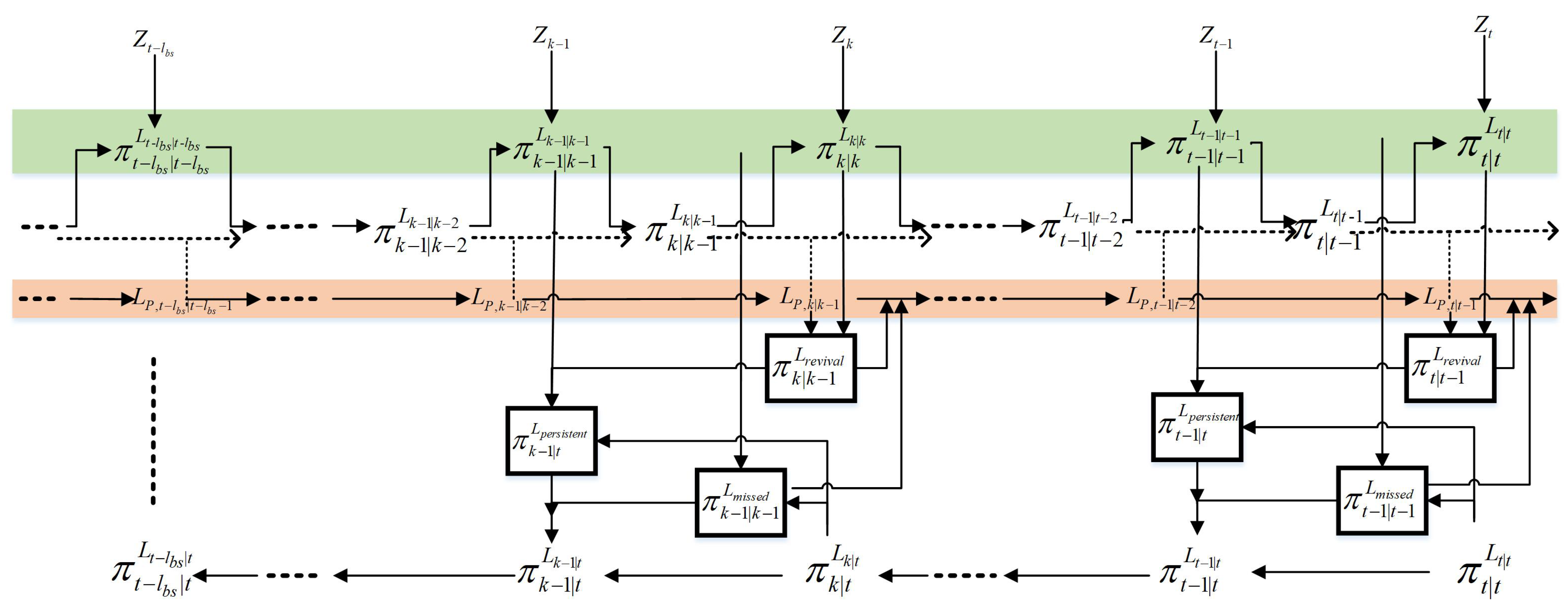
In order to further optimize the state estimation and track extraction of the Labeled RFS trackers, this article proposes a sequential joint state estimation and track extraction algorithm based on label iterative processing which combines the LMB filtering with backward smoothing. The advantages of this algorithm are as follows: (1) It can correctly remove interference in real time and output smooth estimated tracks; (2) It integrates track start determination and processing with label iterative processing, enabling it to sequentially process invalid short-lived targets; (3) It integrates label iterative processing with track continuity processing, enabling it to sequentially process track fracture. Figure 1 shows the processing flowchart and improvement points of the algorithm in this paper. The improvement parts are marked in red boxes in the figure. Finally, by comparing with similar algorithms and analyzing the results, its effectiveness is verified in tracking. Table 1 gives the nomenclature table of all the symbols and notations in the article.
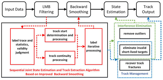
Figure 1.
Algorithm flow of sequential joint state estimation and track extraction based on improved backward smoothing.

Table 1.
Nomenclature table of all the symbols and notations.
The rest of this article is organized as follows. Section 2 first presents the SMC implementation of LMB filter and backward smoothing. Section 3 details the theoretical derivation process and implementation pseudo-code of the proposed algorithm reader’s convenience and replication. Section 4 presents simulation and experimental results to verify the effectiveness of the proposed method. Section 5 introduces the conclusions of the article and future research expectations.
2. The SMC Implementation of LMB Filtering and Backward Smoothing
The Labeled RFS theory represents the state of multiple targets as , where represents the label state of a single target and is the label of target . and are the state set and label set of multiple targets, respectively, which together form the label multi-target state set . And represents the cardinality (number of targets) of the multi-target state, where , , , and are the state space and label space of the targets, respectively.
When the multi-target state obeys an LMB distribution [8], its probability density function (PDF) is expressed as follows:
where is the indicator function of different labels; when the labels in are completely different, , otherwise, ; is the assumed weight; where the mapping makes , ; the assumed weight can be calculated by , where is the inclusion function; when , , otherwise, ; represents the survival probability of the target with label ; for , if , then ; where is the density function of the target , if , then . The above LMB PDF can be equivalently written as .
The standard LMB filtering process [8] (which includes the prediction and update processes) and the SMC implementation of the LMB backward smoothing process [14] are provided below.
2.1. Prediction
The LMB multi-target posterior PDF at time is denoted as , where represents the set of particles of the density function of track , is the particle weight, is the particle state, and is the particle number; Similarly, the set of particles of the newborn LMB multi-target PDF at time can be denoted as . Combining with the LMB filter prediction step, the set of particles of the predicted target PDF can be obtained as
- Predict the set of particles of survival targets :
- Predict the set of particles of newborn targets :
The PDF of the newborn track can be initialized as
where the set of particles simulates the region in state space where target birth events may occur. The set of newborn target particles satisfies a certain distribution, and its particle set can be represented by approximating the predicted PDF of newborn track to particle set . This article adopts the measurement-driven birth approach to generate newborn targets (refer to reference [14] for the specific derivation, which is not repeated here). The LMB distribution of newborn targets at time is determined by measurement at time , with each component corresponding to a measurement value at time . The probability of these newborn targets is represented as
where is the expected number of newborn targets at time ; is the preset maximum value of the newborn probability; is the association probability between measurement and hypothesis, and the larger it is, the lower the probability of the newborn target; and is the assumed association weight at time , provided by Equation (13). The function determines whether a hypothetical weight is associated with the measurement . If associated, add the weight to the association probability. If the measurement is not associated with any assumptions, then . is the subset operation, is the association hypothesis space, is the set of association hypothesis, and .
2.2. Update
The target measurement set at time is denoted as , and the particle set of for updating the multi-target posterior PDF is denoted as .
where
where is the likelihood function, denotes the detection probability of the target , and represents the density function of the clutter. For more details, please refer to [14].
2.3. Backward Smoothing
In order to further improve tracking accuracy, researchers have introduced backward smoothing. Compared with real-time forward filtering, backward smoothing uses all observations at the current time to estimate the state of the past, utilizing more observation information to obtain a more accurate and smoother track. Subsequently, researchers have combined the Labeled RFS theory with smoothing, further expanding and extending the application in state estimation and track output. LMB backward smoothing can efficiently output a smooth track of multiple targets, so this article applies it. The specific theoretical description is provided below.
Assuming that the forward filtering is performed at time , and the smoothed posterior PDF from time to is , then the smoothed posterior PDF from time to is . From the LMB forward filtering, it is known that and both follow the LMB distribution. If follows the LMB distribution, then still follows the LMB distribution [12], which can be expressed as
where
3. A Sequential Joint State Estimation and Track Extraction Algorithm Based on Improved Backward Smoothing
In the process of multi-target tracking, there are often issues such as track fracture and track failure. Most algorithms rely on certain strategies to achieve the goal of track extraction. Common track extraction strategies include:
(1) Saving the remaining tracks that are not used at the current time, so that they can be used as the track head at the next time to start the track.
(2) Deleting tracks that do not have updated points at the current time or have a slightly lower number of track points for multiple consecutive times, which may be caused by noise, clutter or interference.
(3) Deleting tracks with a slightly lower number of track points and inconsistent target characteristics, which may be caused by clutter or interfering/jamming targets.
(4) Sorting the track numbers for confirmed tracks and output tracks.
In order to pursue ultimate tracking performance, these strategies are usually managed and processed in batch mode, which makes the algorithm lose the possibility of real-time processing. For better handling of the track continuity, this article proposes a sequential joint state estimation and track extraction algorithm based on improved backward smoothing based on label iterative processing (Figure 2 shows the framework diagram), which not only can effectively remove outliers and short-lived target tracks using backward smoothing, but also further improves the performance of recovering track fracture to achieve sequential state estimation and track extraction of radar multi-target tracking. The steps are as follows.
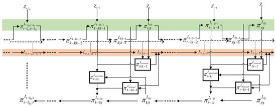
Figure 2.
Algorithm processing framework.
The following should be noted: (a) The starting time of the loop in steps 2 and 4 is different, like “” and “”. (b) Due to the introduction of backward smoothing, in order to facilitate identification, this article uniformly uses the subscript “” to represent the newborn state, the subscript “” to represent the predicted state, the subscript “” to represent the updated/posterior state, and the subscript “” to represent the smoothed state. Please pay attention to this distinction when reading. (c) In the backward smoothing processing loop, a single cycle plays the role of smoothing the survival-target state and eliminating interference, and multiple cycles play the role of using the target state at the latest moment to repeatedly correct the target state within the smoothing window, including completing the target state in step 4, thus improving the tracking performance at the track fracture. (d) There are three main loops in the algorithm, which are nested within each other. Please pay attention to the internal processing logic. (e) Since the output of the algorithm is obtained through parameter estimation and extraction based on the result of backward smoothing, the final determination result obtained by the algorithm is delayed by steps.
Loop begins.
Step 1: Prediction
Suppose the posterior PDF at time is . In the prediction step of the proposed method, in addition to the prediction process for the survival target and the newborn target process, in order to obtain the target state at the track fracture, the proposed algorithm uses the predicted state of the missed target at the previous time in the backward smoothing processing range to recursively obtain its predicted state at the next time, which is used as the basis for track recovery. Here, the predicted state set that includes the hypothetical predicted state set of the status-pending label set is called the enhanced predicted PDF.
Using Equations (3)–(6), obtain the predicted PDF of the survival target at time :
Using Equations (7)–(9), obtain the predicted PDF of the newborn target at time :
Using the following steps to obtain the hypothetical predicted PDF of the status-pending label set at time :
where the single-target state transition function , the survival probability of the status-pending target , and the stochastic process noise are all set according to the prediction of the survival target.
Combining with the above derivation process, the enhanced predicted PDF at time is obtained as follows:
Step 2: Update
Assuming that the measurement set is obtained at time , then according to Equations (10)–(17), the updated/posterior PDF is .
Step 3: Improved backward smoothing
Assuming the backward smoothing step length is , the following are the improved steps for backward smoothing in this article:
(1) Firstly, the posterior PDF of the persistent target (existing at time and simultaneously) is obtained by smoothing, and the smoothed posterior PDF at the next time is obtained from the smoothed posterior PDF at the previous time by backward smoothing in Equations (19)–(22).
(2) By tracing and counting the target label, outliers and the status-pending target are determined based on the label history, and the corresponding state and label of invalid targets are removed.
First, the vanishing label set is obtained at time , and then label tracing and statistics of the vanishing label set are used to determine the status of the labels. The determination principle is as follows:
In the backward smoothing process at time , the number of occurrences of each label in the vanishing label set from time to (here, time is used to instead of time , emphasizing the full utilization of history information before and after the label) is counted, and it is determined whether the number of the historical occurrences of each label exceeds the effective number . If not, it is determined to be an outlier or an invalid short-lived target (here, it is assumed that the number of historical occurrences of an outlier does not exceed 1, and the number of historical occurrences of the invalid short-lived target does not exceed ). If it exceeds this number, it is determined to be a missed label set . The specific discrimination formula is as follows:
where represents the total number of occurrences of label at time . Finally, the missed label set is used to correct the backward smoothing result.
(3) Use the following equation to obtain the preliminarily corrected smoothed posterior PDF .
(4) According to , the parameter state is extracted using the K-means clustering algorithm [21] to obtain ; represents the extracted state of the label , and represents the set of estimated labels corresponding to all estimated target states at time .
Step 4: Track filling
When there is a duplicate target in the status-pending label set , fill its hypothetical predicted PDF at the fracture.
Step 5: Update and obtain the status-pending label set for the next moment
where is defined as above, and , is the track start determination length.
Step 6: Normalize weight, resampling, and track pruning
Loop ends.
It should be emphasized here that the algorithm output results are extracted from the parameter estimation of the backward smoothing output results. Because of this, this article achieves the above functions by performing traceback processing on the labels in smoothing processing, which allows the algorithm to correct the filled tracks using the backward smoothing process.
Computational complexity: The main computational cost of the processing algorithm proposed in this article comes from LMB backward smoothing. The computational complexity of backward smoothing is , where is the backward smoothing step length, is the number of tracks, and is the number of particles approximated by PDF particles for each track. The specific source is the four for loops in back smoothing. The computational complexity of the two parallel inner for loops is , and then multiplied by the two outers for loops to obtain the final computational complexity of .
In order to facilitate readers’ understanding and replication, the pseudo-code of the proposed Algorithm 1 is provided below.
| Algorithm 1: Pseudo-Code |
| Input: ,; |
| Output: |
| ( is the number of simulations) |
| according to (3)–(6) and (23)–(27) |
| according to (10)–(17) |
| according to (19)–(22) |
| Normalize weight, resampling, and track pruning. |
4. Experiment Analysis
This article takes the tracking of UAV targets under the pulse Doppler (PD) radar system as the research background and combines this with the actual background parameters to verify the effectiveness of the proposed algorithm through simulation data and measured data. The radar’s carrier frequency is , the pulse repetition frequency is , the distance sampling interval is , and the number of distance sampling points is . The algorithm is SMC implementation, and the number of particles is set to .
The wavelength of the radar can be calculated from its basic parameters as , and the maximum unambiguous velocity is (the range of unambiguous velocity is from 0 to ). The maximum unambiguous range is . To avoid the effects of velocity and range ambiguity, this article refers to the above data to set the target velocity and observation scenario.
Scenario parameter setting: The scenario setting in this article are the same as those in [18] and the source of the measured data. The observation area is set to with reference to the actual scenario setting. In this article, we compromise and choose a coherent accumulation time of , which is 800 for coherent accumulation. At this point, the speed accuracy can reach under accurate focusing, fully meeting the tracking requirements.
State transition equation: In this paper, a discrete acceleration model is considered as the state transition equation, and the state variable of a single target is represented as , where is the distance, is the radial velocity, and is the radial acceleration. The state transition equation is as follows:
where is the state noise of , describes the random process noise in the particle motion process in Equations (5) and (6), and the state transition matrix and noise transformation matrix are, respectively,
The measurement distance and speed are noisy, and the measurement equation is as follows:
where the measurement noise is , . and are the approximate variance of the target’s distance and speed, respectively.
Target measurement noise: Calculate the approximate variance of the target distance and velocity from the measured data, and select and . The detection probability of the target is based on the actual scenario settings. The Clutter density function follows the Poisson distribution, and the number of clutters in the observation scene is given in the subsequent parameter settings.
Target motion noise: Based on the analysis of the measured data, the process noise standard deviation for each time step can be set to , and the probability of the survival target and the status-pending target are both set to .
Newborn-target probability density parameter settings: and can be set. Considering that the main processing is carried out during the tracking stage, the measurements in the simulation experiment are obtained after the CFAR detection value is condensed by the plot. The estimated value is the filtering output value of the LMB smoother. In addition, the experiment uses measurement-driven target birth to generate new targets. Assuming that follows a Gaussian distribution, the variance of the Gaussian distribution is equal to the variance of the observation noise , and the mean is equal to the value of the state corresponding to the observation predicted one step forward, which is expressed as follows:
This article uses the Optimal Sub-Pattern Assignment (OSPA) distance error to evaluate the tracking performance of the proposed algorithm, which is defined as follows:
where if , , and when , . and are finite non-empty subsets of the unlabeled estimated state and real state of targets, respectively. and are the cardinality of states; , represents the Euclidean distance, and represents all possible permutations on the set ; the parameter is the truncation distance, which controls the weight of cardinality error and location error. The greater , the more emphasis OSPA places on the influence of cardinality error. The parameter determines the sensitivity to outliers. In this article, we set and .
On the basis of the above, the OSPA distance error is further divided into OSPA location error component and OSPA cardinality error component to separately evaluate tracking accuracy (state estimation) and tracking integrity (cardinality estimation), defined as
In addition, due to the use of Monte Carlo simulation in this article, all the OSPA errors provided are the average values in the time dimension. And for the convenience of comparison, the average OSPA error is accumulated and summed over time to obtain a single value of the total OSPA error. In this article, the experiment is carried out in the form of Monte Carlo simulation, the simulation times are set to 100, and the final experimental results are analyzed.
4.1. Description of Processing Effect
4.1.1. Track Start Determination and Processing
The algorithm proposed in this article can effectively discriminate outliers and invalid short-lived targets by tracing and statistics of target labels, and then eliminates the above interferences through backward smoothing to achieve sequential track start determination and processing.
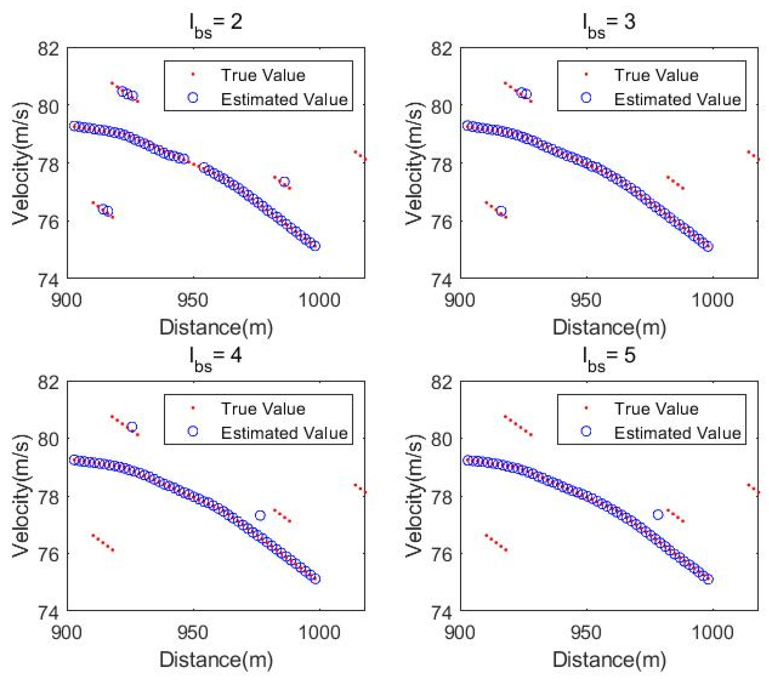
First, track start processing is performed after completing track start determination, using backward smoothing to eliminate interferences like outliers and invalid short-lived targets, and the removal effect depends on the backward smoothing step length . To elaborate, this article conducts simulations of the length of different backward smoothing step length on the processing of short-lived tracks. The scene setting is provided in Table 2 and the processing effect is shown in Figure 3a. In order to visually demonstrate the processing effect, the experiment avoids interference from motion noise, measurement noise, and clutter.
Table 2.
Scene setting.
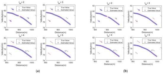
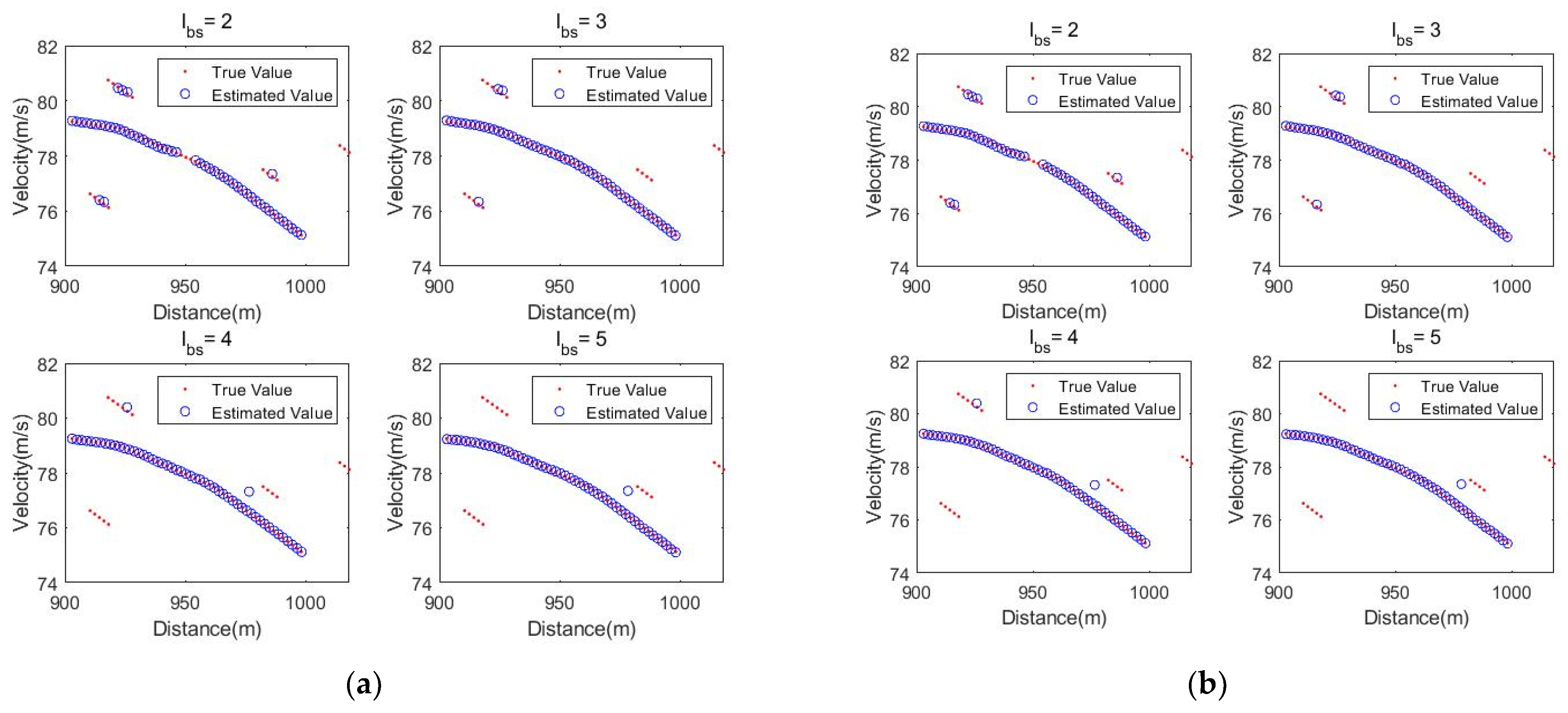
Figure 3.
(a) Track start processing results under different backward smoothing step lengths; (b) processing result under different track start determination length.
Figure 3a contains a normal target (T1) and four jamming targets (J1, J2, J3, J4) with point lengths of 3, 4, 5, and 6, respectively. When processed with backward smoothing step lengths of 2, 3, 4, and 5, respectively, the four jamming targets are removed to varying degrees, and the number of removed jamming points depends on the backward smoothing step length. From the experimental result, it can be seen that when the backward smoothing step length is set to , the track of the four jamming targets can be perfectly removed, achieving the expected effect.
The above experiment demonstrates that the track start processing depends on backward smoothing, while track start determination is determined by the length of the track start determination. On the basis of the above simulation, further analysis is conducted on the processing effect of the algorithm under different track start determination lengths. At this time, the track start determination length is taken as , and the backward smoothing step length is taken as . From Figure 3a, it can be seen that the backward smoothing step length can effectively remove the jamming targets with lengths of 2, 3, 4, and 5 in the scene, while the track start determination length will determine whether the target is a jamming target or a target that does not meet the track start length based on the parameter setting, so as to eliminate it using backward smoothing. The simulation results are shown in Figure 3b.
From the experimental results above, it can be seen that as the track start determination length gradually increases, the jamming targets 1–4 are gradually eliminated, while the normal targets are not affected. The above results verify the track initiation determination and processing effect of the proposed algorithm.
4.1.2. Track Continuity Processing
Another innovation of this article is the fusion of track continuity processing and backward smoothing. This fusion not only fills the target hypothetical predicted PDF as the posterior PDF when the target reappears (detected again), but also modifies it through backward smoothing. Compared to interpolating the estimated points at the fracture through interpolation [18], this approach can be implemented in a sequential manner and also improves tracking performance, which will be further verified in subsequent analysis. In order to further illustrate the track continuity processing of this algorithm, this article conducted simulations according to the scene parameter settings provided in Table 3, which included targets with varying degrees of fracture. The experimental results are simulated under different track continuity processing lengths . In addition, the track start determination length is set to . In this simulation, in order to visually demonstrate the problem, the experimental factors such as motion noise, measurement noise, and clutter interference are also avoided.
Table 3.
Scene setting.
The normal target in the simulation scenario includes track fractures with the length of 3, 4, and 5. It can be seen from the experimental results in Figure 4 that, as the track continuity processing length gradually increases, the three different length track fractures are recovered one by one. The above results verify the effectiveness of the proposed algorithm for track continuity processing.
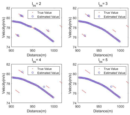
Figure 4.
Processing result under different track continuity processing length.
4.1.3. The Influence of Backward Smoothing Step Length on Tracking Performance
In this simulation, interference is considered, and the scene setting is provided in Table 4. Here, the backward smoothing step lengths are .
Table 4.
Scene setting.
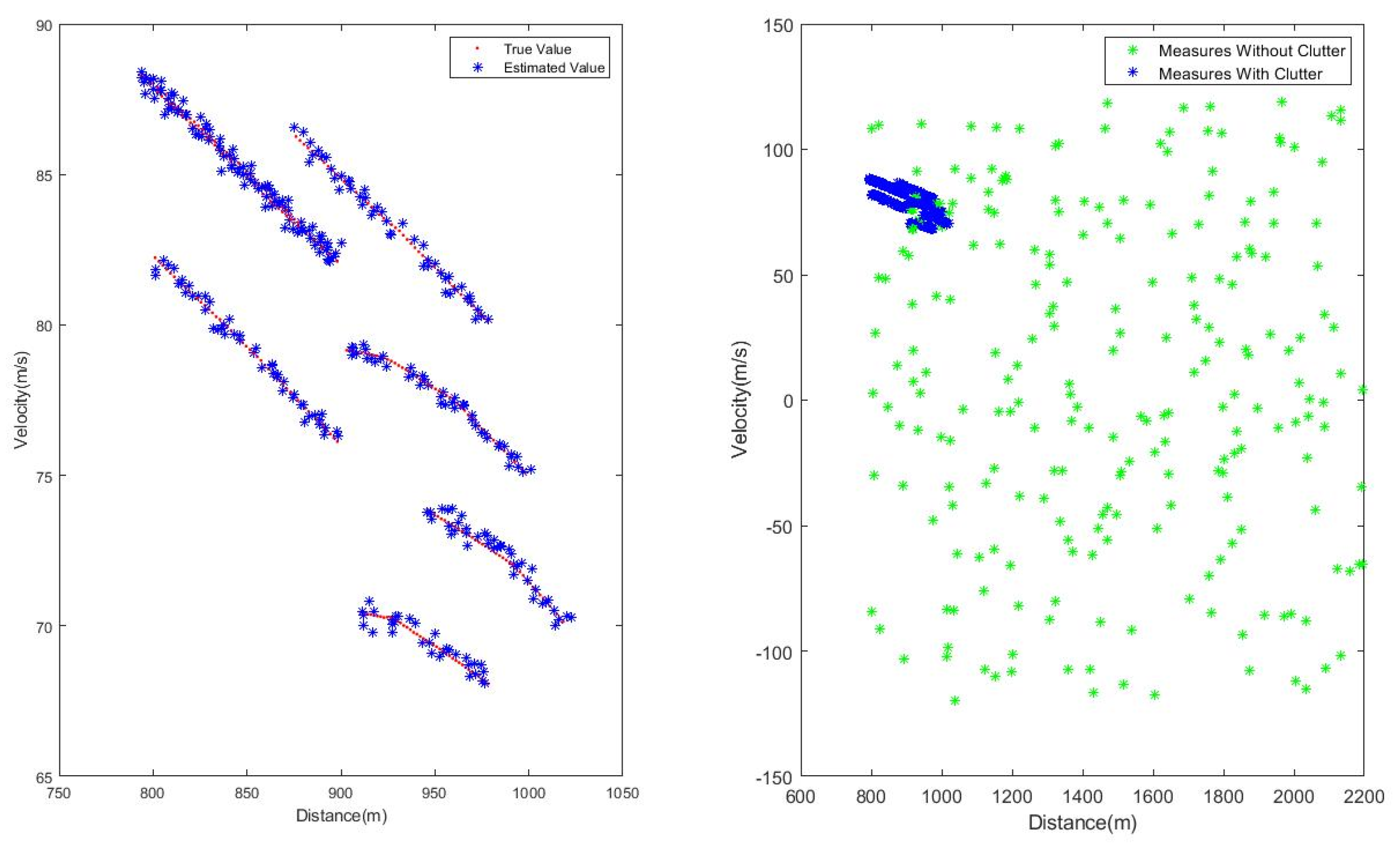
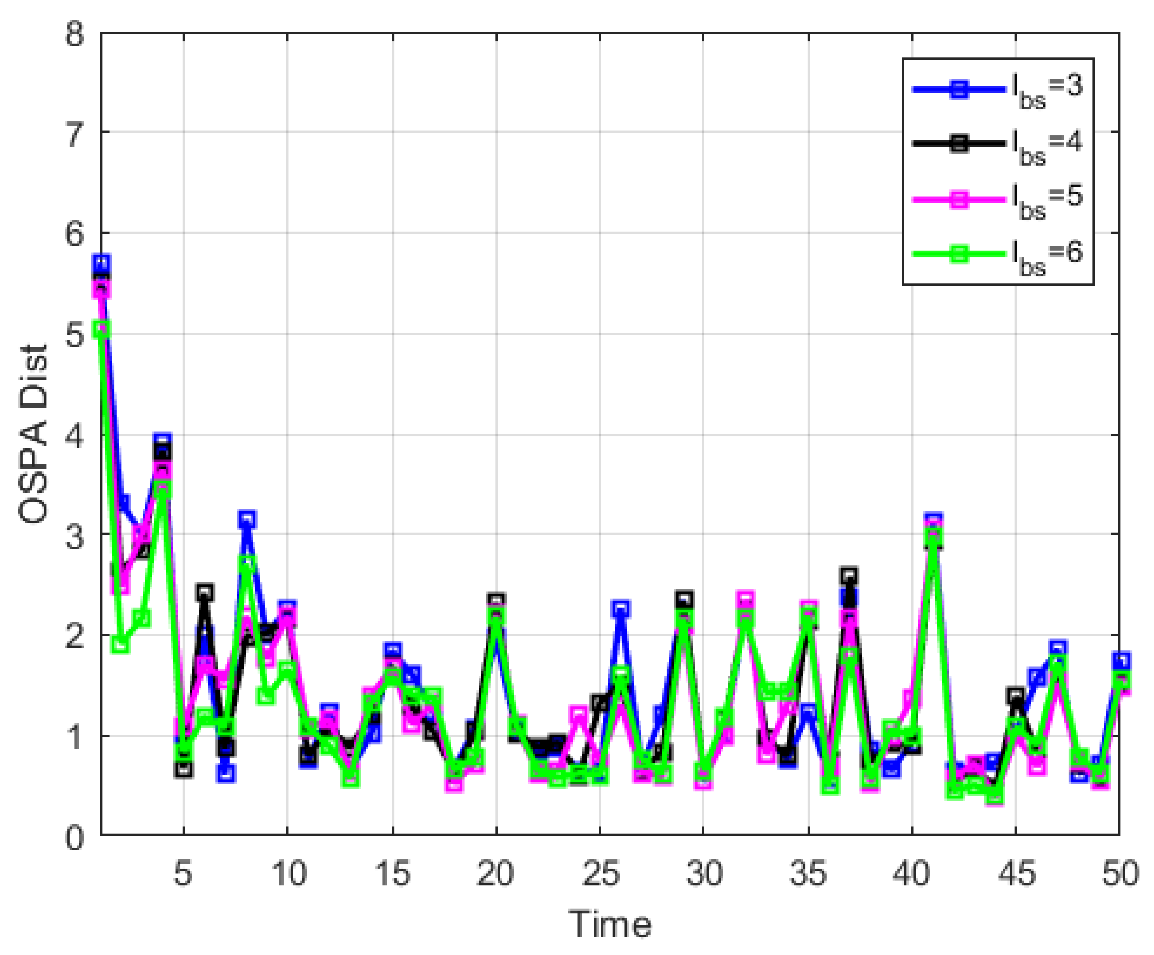
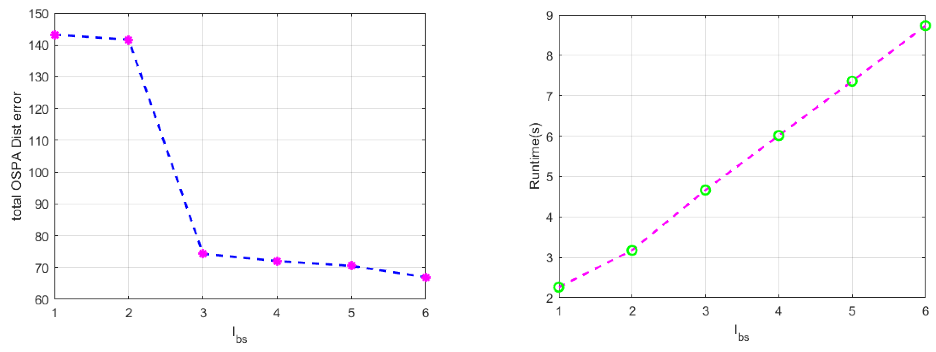
Figure 5 gives the real state value and measured value of the simulated scene. Figure 6 and Figure 7 show the specific experimental results. In the algorithm proposed in this article, the step length of backward smoothing is directly related to the length of short-lived targets and track fractures that the algorithm can handle, and also directly affects the estimation performance of the target state. Figure 6 shows the average OSPA distance (referring to the average of multiple results under Monte Carlo simulation) obtained under different backward smoothing step lengths while ensuring the normal processing of short-lived targets and recovering track fractures. Figure 7 shows the total OSPA distance (sum of the average OSPA distances over time) and runtime under different backward smoothing step lengths. Combining Figure 6 and Figure 7, it can be summarized that backward smoothing is beneficial for improving tracking performance, but it is not friendly to computation burden. Therefore, in the processing process, the setting of the backward smoothing step length should be considered as a compromise, and the runtime and tracking performance should be comprehensively considered.
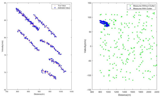
Figure 5.
Real state value and measured value.
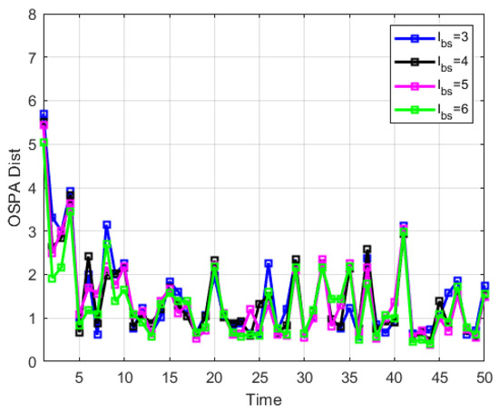
Figure 6.
Average OSPA distance error under different backward smoothing step lengths.
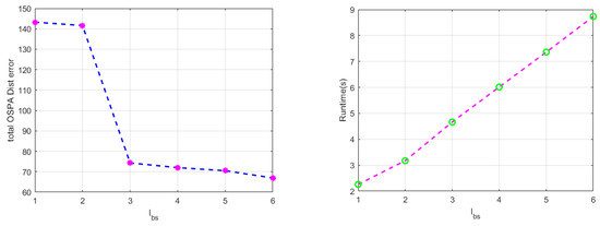
Figure 7.
Total OSPA distance error and runtime under different backward smoothing step lengths.
4.2. Multi-Target Scene Simulation
To further verify the tracking performance of the proposed algorithm, an experiment was conducted with the scene setting as shown in Table 5. The experiment included 3 targets, 6 short-lived jamming targets, and clutter. The simulation results are shown in Figure 8, Figure 9, Figure 10 and Figure 11.
Table 5.
Scene setting.
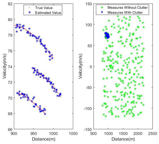
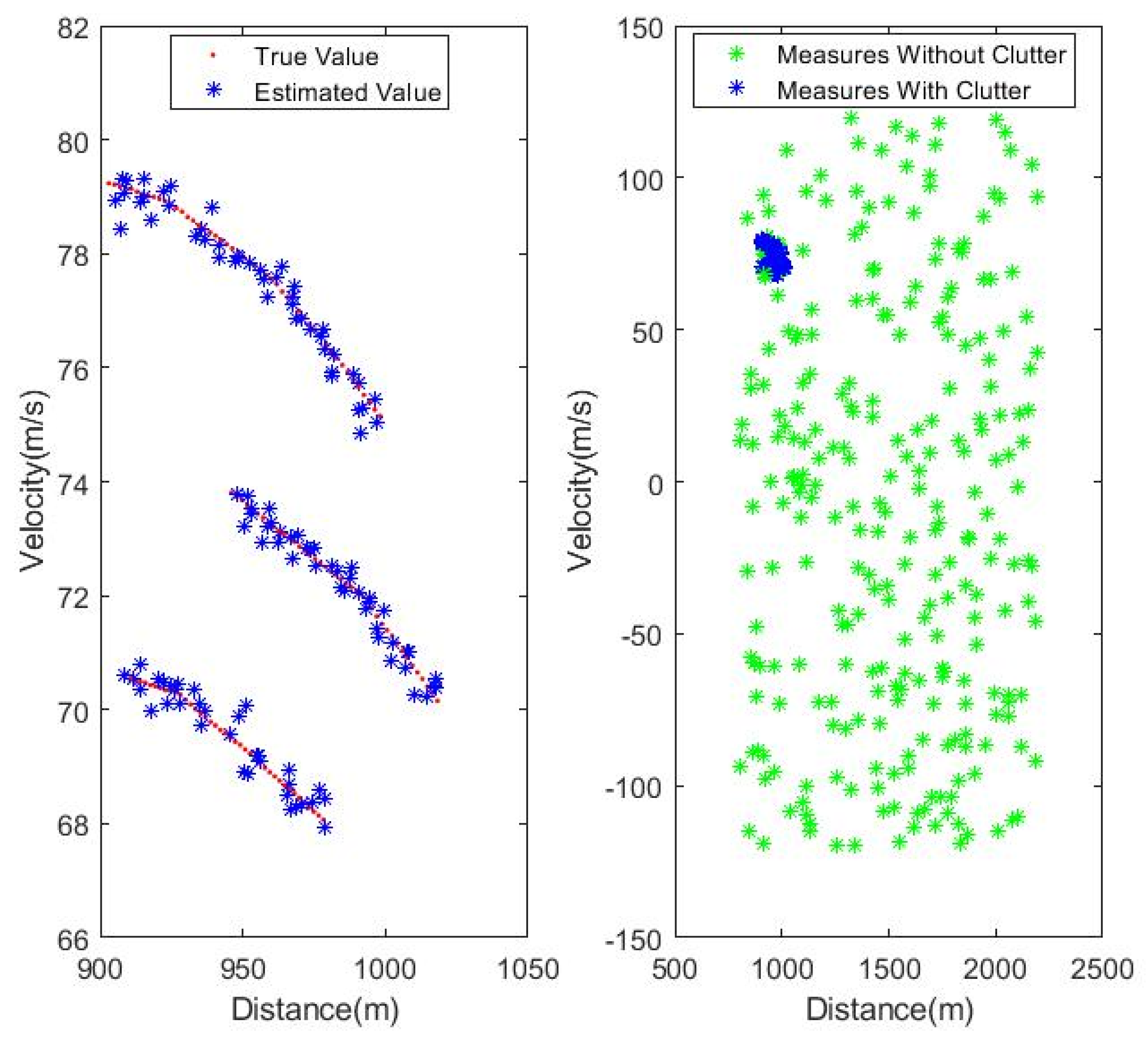
Figure 8.
Real value and measured value.
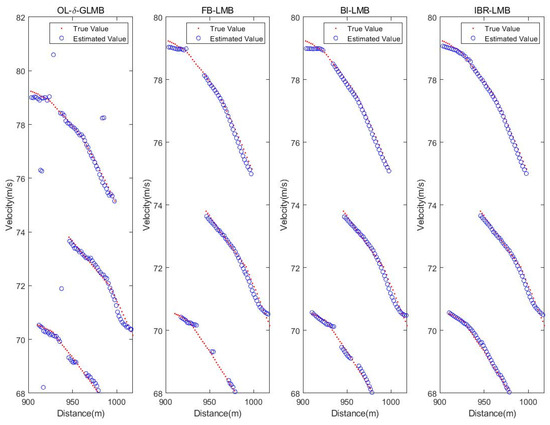
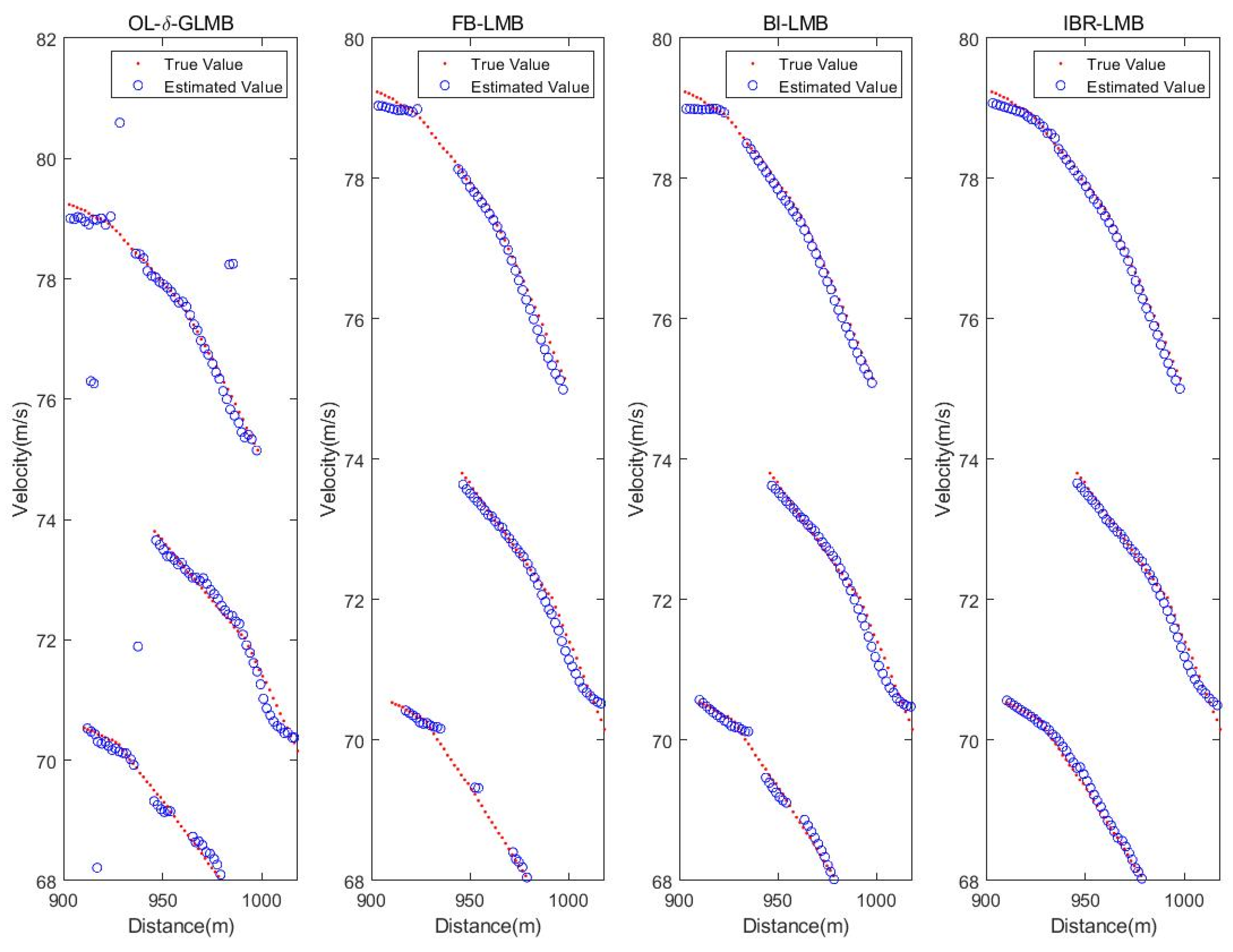
Figure 9.
Multi-target simulation result of four algorithms.
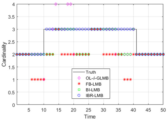
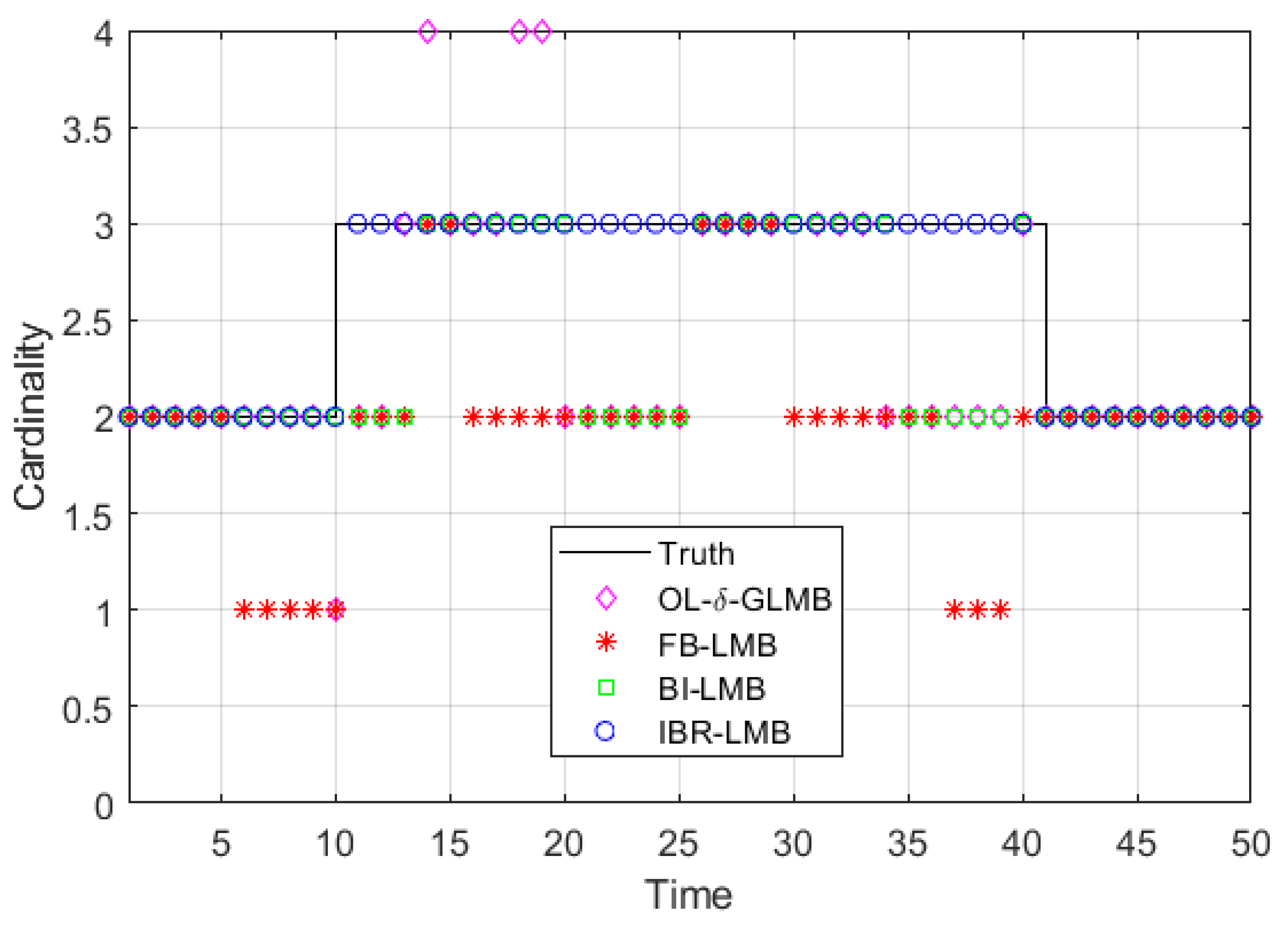
Figure 10.
Average cardinality-estimation result of four algorithms.
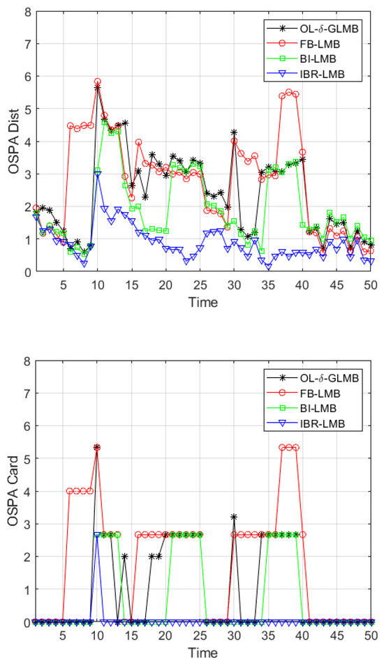
Figure 11.
Average OSPA distance and cardinality error of four algorithms.
Ref. [11] provides a detailed comparison between four smoothers including LMB smoother [12], δ-GLMB-A smoother [22], δ-GLMB filter, and the proposed OL-δ-GLMB smoother. Ref. [14] thoroughly compares the processing performance of MB smoother, CB-MeMBer filter, PHD filter, PHD smoother, LMB filter, and the proposed FB-LMB smoother. Here, the proposed algorithm (IBR-LMB smoother) is compared with OL-δ-GLMB smoother, FB-LMB smoother, and Backward-Interpolation LMB (BI-LMB) smoother [19] to verify the effectiveness.
For the four smoothers (FB-LMB, OL-δ-GLMB, BI-LMB, IBR-LMB), the reasons for the distortion points in Figure 10 stem from three aspects: outlier removal, short-lived track removal, and track continuity processing. First, to explaining these three aspects one by one: outlier removal is to remove outliers using backward smoothing under the control of backward smoothing step length; short-lived track removal is also to process short-lived tracks using backward smoothing processing combined with track start determination; track continuity processing is to use backward smoothing to reasonably recover track fractures. Among the four smoothers, except for the proposed IBR-LMB smoother, the other three methods only have partial capabilities.
FB-LMB smoother has an ability to remove outliers using backward smoothing, but there is a problem of erroneous removal due to missed detection, and it does not have the ability to process track continuity. Therefore, combined with the multi-target simulation scenario settings provided in Table 5, it can be seen that FB-LMB smoother can effectively remove outliers, so all distorted points are free of the interference of outliers and short-lived tracks. In the processing result of FB-LMB smoother given in Figure 10, points 6, 7, 8, 9, and 10 are erroneously removed due to missed detection of target T3 at time 11–12 under the influence of the smoothing step length, while points 11 and 12 are caused by missed detection of target T3 itself. Point 13 is due to the thresholding of the first point at the beginning of the track due to its low initial survival probability. Points 16, 17, 18, 19, and 20 are also erroneously removed due to missed detection of target T3 at time 21–24 under the influence of the smoothing step length, while points 21, 23, and 24 are caused by missed detection of target T3 itself. Point 30, 31, 32, 33, and 34 are also erroneously removed due to missed detection of target T1 at time 35–38 under the influence of the smoothing step length. Points 35–38 are affected by missed detection of target T3 itself and point 36 may also be affected by unstable determination due to ineffective processing of outliers. Points 37 and 38 are erroneously removed due to the algorithm’s assumption of missed detection of target T1 at 41, while point 39 is erroneously removed due to the thresholding of the first point at the beginning of the track due to its low initial survival probability, and target T1 is not measured at 41, which the algorithm assumes to be a missed detection. Point 40 is erroneously removed due to the algorithm’s assumption of missed detection of target T1 at 41.
BI-LMB smoother has an ability to remove outliers using backward smoothing and corrects the problem of erroneous removal caused by missed detections. However, it does not have the ability to process track continuity. Therefore, compared to FB-LMB smoother, BI-LMB smoother has distortion points only at targets T1 in time 11–12, targets T3 in time 21–24 and 35–38 due to missed detections, and at points 13, 25, and 39 due to the threshold removal of the first point at the start of the trajectory due to its low survival probability.
OL-δ-GLMB smoother only has an ability to remove outliers and incomplete short-lived tracks in one-step processing, but it still has the problem of one-step error removal due to missed detection. In addition, it does not have the ability to process track continuity. Here, we first analyze the removal results of short-lived tracks J1-J6 by OL-δ-GLMB smoother: Due to the one-step smoothing of OL-δ-GLMB smoother, it cannot effectively remove short-lived tracks like other smoothers. Due to its one-step smoothing step length, its ability to remove short-lived tracks is limited. In addition, due to the threshold removal effect of the first point in the track initiation, the result is that J1 is normally removed, but point 13 in J2 is not removed, and points 18 and 19 in J3 are not removed. Point 30 in J4 and J5 is not removed and point 40 in J6 is not removed. Therefore, further analysis is conducted based on the above results. Point 10 is due to one-step error removal caused by missed detection of target T3 in time 11–12. Points 11 and 12 are due to missed detection of target T3 itself in time 11–12. In addition, it should be noted that although point 13 appears to be undistorted, it is actually retained due to the one-step smoothing of OL-δ-GLMB smoother, which leads to the removal of short-lived track J1 at point 13. However, there is an impact of threshold removal due to the low survival probability of the first point in the track initiation, which makes point 13 appear undistorted but actually have a problem. Point 18 and 19 are due to the removal of short-lived track J3 at points 18 and 19. Point 20 is due to one-step error removal caused by missed detection of target T3 in time 21–24. Points 21–24 are due to missed detection of target T3 itself in 21–24. Point 34 is due to one-step error removal caused by missed detection of target T3 in points 35–38. Points 35–38 are due to missed detection of target T1 itself in 35–38. Point 39 is due to threshold removal due to the low survival probability of the first point in the track initiation.
As shown in Figure 8, it can be seen that the proposed IBR-LMB smoother output track is smoother and more complete compared to other algorithms. Figure 11 show the average OSPA distance and cardinality errors of four algorithms. Table 6 presents the total OSPA errors of four algorithms. From the above results, it can be seen that the proposed IBR-LMB smoother outperforms other algorithms in cardinality-estimation performance due to eliminating interferences and recovering track fractures. Eventually, it can be concluded that the proposed IBR-LMB smoother is superior to the other three smoothers, verifying its effectiveness.
Table 6.
Total OSPA errors of four algorithms.
4.3. Verification of Measured Data
In the end, the proposed algorithm is verified by the measured data. The actual scenario and parameter setting are provided in Table 6. Track start determination length is set to 3. Figure 12, Figure 13 and Figure 14 and Table 7 provide the experimental results. Here, the results of the four algorithms are also compared and analyzed.
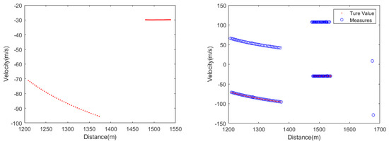
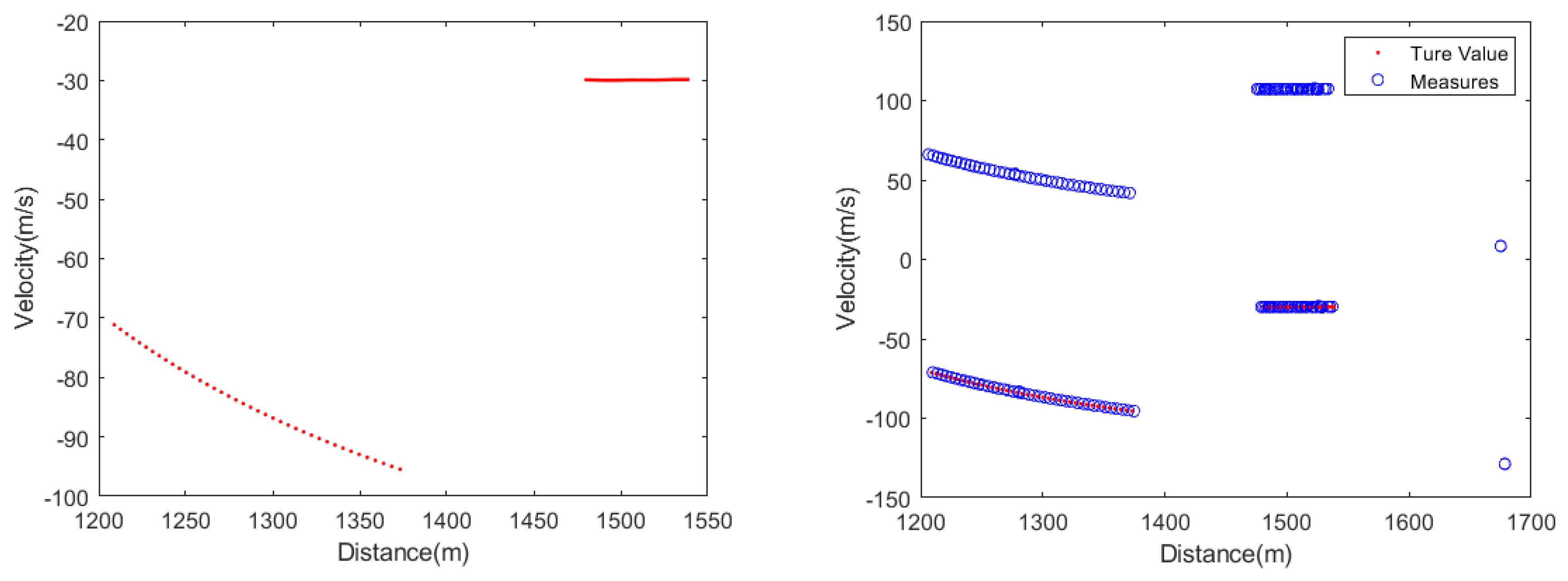
Figure 12.
Real state value and measure value of measured data.
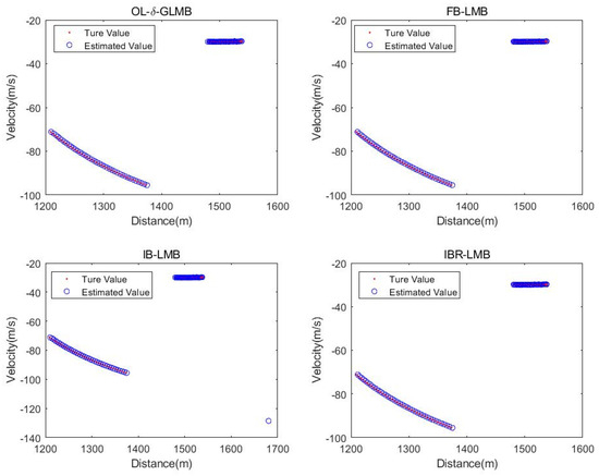
Figure 13.
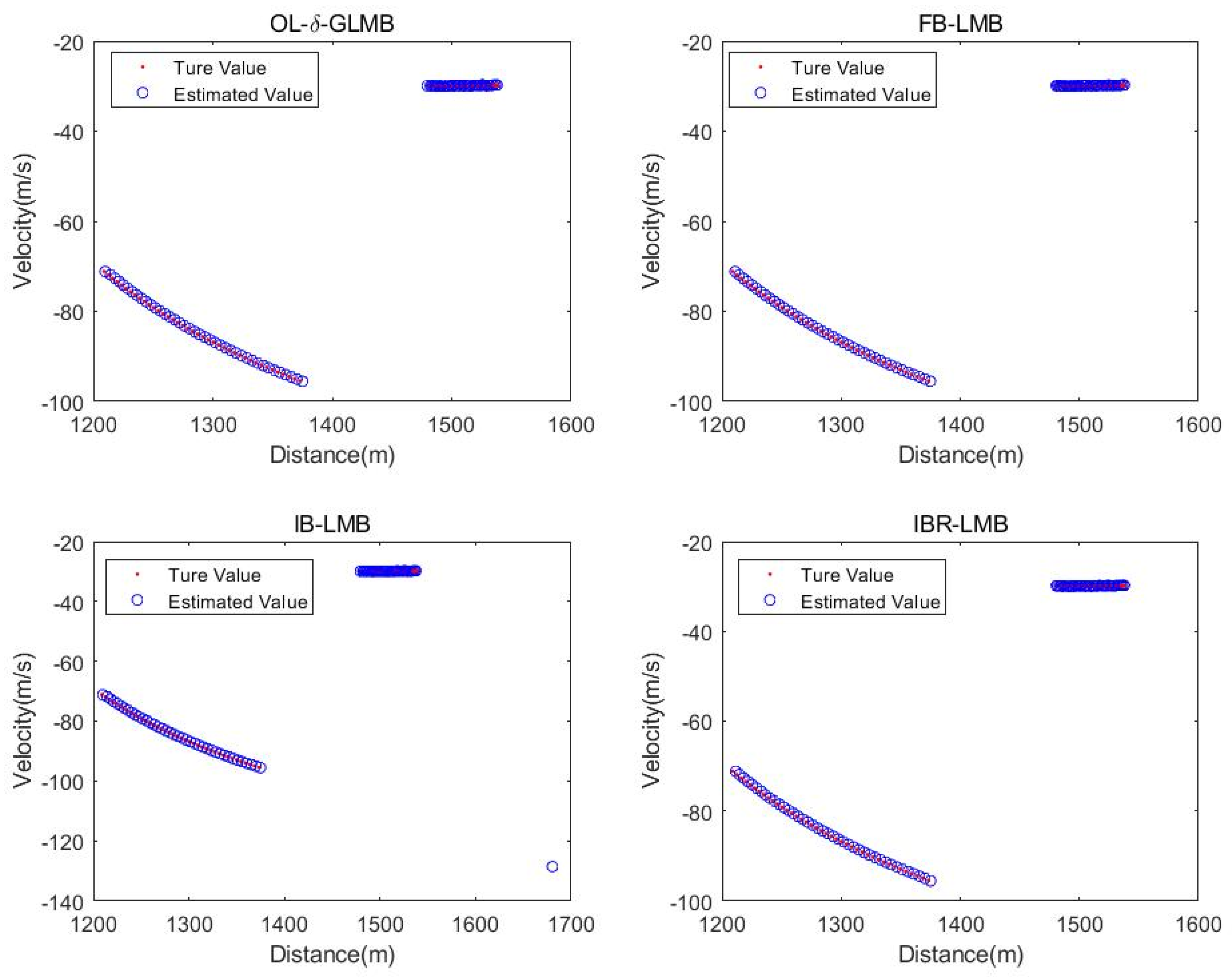
The processing result of four algorithms for measured data.
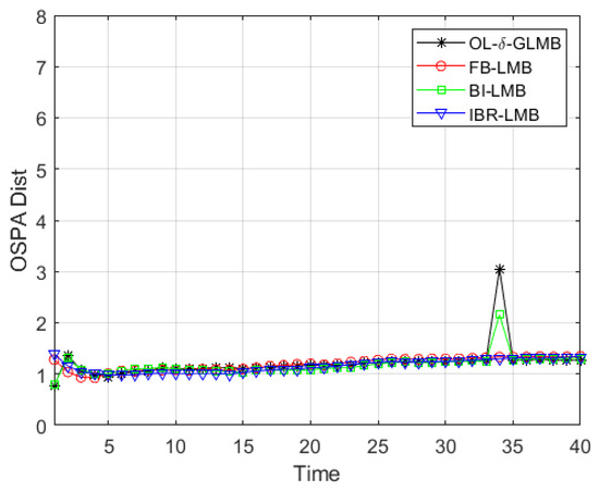
Figure 14.
Average OSPA distance and cardinality error of four algorithms in measured data.
Table 7.
Scene setting.
The measured data contains two targets, and their true target state values are shown in Figure 12. Firstly, as shown in Figure 14, the proposed algorithm still has a better OSPA distance error compared to other smoothers, which can also be seen from the specific total OSPA distance error value given in Table 8. In addition, it should be noted that from the true target state values and measured values provided in Figure 12, the measured data used in this article is relatively smooth, which makes the tracking performance of the proposed algorithm not much different from other algorithms, which can be seen from Figure 13, but it is still the optimal algorithm (based on the results of Monte Carlo simulation, the simulation times is 100). Combined with multi-target scene simulation in Section 4.2, it can be seen that with the aggravation of interferences such as motion noise, measurement noise, clutter, etc., the proposed algorithm has more obvious advantages.
Table 8.
The total OSPA errors of four algorithms.
5. Conclusions
This article aims to improve the performance of state estimation and track extraction ability for multi-target tracking in radar. Based on LMB filtering, combining with backward smoothing, a sequential joint state estimation and track extraction processing algorithm based on label iterative processing is proposed. Numerical analysis results show that the proposed algorithm can effectively eliminate outliers and short-lived targets, improve the performance of target cardinality and state estimation to a certain extent, and effectively recover track fractures and improve the tracking performance at track fractures. During the research process, it was found that using label iterative processing helps Labeled RFS filters/smoothers to achieve sequential processing of tracks, which is of great significance for conventional algorithms that use batch processing and do not have track output to solve the problem of track initiation and continuity. Therefore, it is proposed to further combine the existing more mature Labeled RFS algorithms to explore how to improve the performance of maneuvering multi-target tracking performance through label iterative processing, and introduce mature fast processing methods from a theoretical level to reduce the computational burden of Labeled RFS filters/smoothers, so as to promote its application in practical engineering.
Author Contributions
J.Z., Z.Z. and K.L. designed the research. J.Z. processed the data and drafted the manuscript. R.Z., S.L. and L.B. helped organize the manuscript. J.Z. and R.Z. revised and finalized the article. All authors have read and agreed to the published version of the manuscript.
Funding
This work was supported in part by the National Natural Science Foundation of China (NSFC) under grant no. 62271491 and 62001486.
Data Availability Statement
Data are contained within the article.
Acknowledgments
The authors would like to acknowledge their colleagues and teachers who participated in research activities and contributed to the development of some of the ideas and results presented in this article.
Conflicts of Interest
The authors declare no conflict of interest.
References
- Bar-Shalom, Y.; Willett, P.; Tian, X. Tracking and Data Fusion: A Handbook of Algorithms; YBS Publishing: Storrs, CT, USA, 2011. [Google Scholar]
- Blackman, S.; Popoli, R. Design and Analysis of Modern Tracking Systems; Artech House Publishers: Boston, MA, USA, 1999. [Google Scholar]
- Mahler, R.P.S.; Ebrary, I. Statistical Multisource-Multitarget Information Fusion; Artech House Publishers: Boston, MA, USA, 2007. [Google Scholar]
- Mahler, R.P.S. Multi-target Bayes Filtering via First-Order Multi-target Moments. IEEE Trans. Aerosp. Electron. Syst. 2003, 39, 1152–1178. [Google Scholar] [CrossRef]
- Mahler, R. PHD Filters of Higher Order in Target Number. IEEE Trans. Aerosp. Electron. Syst. 2007, 43, 1523–1543. [Google Scholar] [CrossRef]
- Vo, B.-T.; Vo, B.-N.; Cantoni, A. The Cardinality Balanced Multi-Tar-get Multi-Bernoulli Filter and Its Implementations. IEEE Trans. Signal Process. 2009, 57, 409–423. [Google Scholar]
- Vo, B.-T.; Vo, B.-N. Labeled Random Finite Sets and Multi-Object Conjugate Priors. IEEE Trans. Signal Process. 2013, 61, 3460–3475. [Google Scholar] [CrossRef]
- Reuter, S.; Vo, B.-N.; Dietmayer, K. The Labeled Multi-Bernoulli Filter. IEEE Trans. Signal Process. 2014, 62, 3246–3260. [Google Scholar]
- Beard, M.; Vo, B.-T.; Vo, B.-N. Generalized Labelled Multi-Bernoulli Forward-Backward Smoothing. In Proceedings of the 2016 19th International Conference on Information Fusion (FUSION), Heidelberg, Germany, 5–8 July 2016; pp. 688–694. [Google Scholar]
- Vo, B.-N.; Vo, B.-T. A Multi-Scan Labeled Random Finite Set Model for Multi-Object State Estimation. IEEE Trans. Signal Process. 2019, 67, 4948–4963. [Google Scholar] [CrossRef]
- Liang, G.; Li, Q.; Qi, B.; Qiu, L. Multi-target Tracking Using One Time Step Lagged Delta-Generalized Labeled Multi-Bernoulli Smoothing. IEEE Access 2020, 8, 28242–28256. [Google Scholar] [CrossRef]
- Liu, R.; Fan, H.Q.; Xiao, H.T. A Forward-Backward Labeled Multi-Bernoulli Smoother. In Proceedings of the 16th International Conference on Distributed Computing and Artificial Intelligence, Avila, Spain, 26–28 June 2019; pp. 244–252. [Google Scholar]
- Liu, R.; Fan, H.Q.; Li, T.C.; Xiao, H. A Computationally Efficient Labeled Multi-Bernoulli Smoother for Multi-Target Tracking. Sensors 2019, 19, 4226. [Google Scholar] [CrossRef] [PubMed]
- Liu, R. Research on Radar Target Tracking with Labeled Random Finite Sets. Ph.D. Thesis, National University of Defense Technology, Changsha, China, 2020. (In Chinese). [Google Scholar]
- Qi, L.; Wang, H.; Xiong, W.; Dong, K. Track Segment Association Algorithm Based on Multiple-Hypothesis Models with Prior Information. Syst. Eng. Electron. 2015, 37, 732–739. [Google Scholar]
- Zeng, X. Multi-Sensor Vessel Target Tracking and Fusion Algorithm. Master’s Thesis, Inner Mongolia University, Inner Mongolia, China, 2022. [Google Scholar]
- Zhou, S. Research on Target Track Segment Association Method Based Gaussian. Master’s Thesis, Hangzhou University of Electronic Science and Technology, Hangzhou, China, 2022. [Google Scholar]
- Liang, P.; Liu, R.; Chen, X.; Shang, Z.; Yi, T.; Lu, D. Radar Weak Target Tracking Based on LMB Smoothing. Aero Weapon 2021, 28, 80–85. [Google Scholar]
- Zhao, J.; Zhan, R.; Zhuang, Z.; Li, K.; Deng, B.; Peng, H. An Improved Backward Smoothing Method Based on Label Iterative Processing. Remote Sens. 2023, 15, 2438. [Google Scholar] [CrossRef]
- Zhao, H. A Study for Radar Multi-Target Tracking Algorithm Based on Random Finite Set. Master’s Thesis, Xi’an University of Electronic Science and Technology, Xi’an, China, 2020. [Google Scholar]
- Anil, K.J. Data clustering: 50 years beyond K-means. Pattern Recognit. Lett. 2010, 31, 651–666. [Google Scholar]
- Li, Q.-R.; Qi, B.; Liang, G.-L. Approximate Bayes Multi-Target Tracking Smoother. IET Radar Sonar Navigat. 2019, 13, 428–437. [Google Scholar] [CrossRef]


Disclaimer/Publisher’s Note: The statements, opinions and data contained in all publications are solely those of the individual author(s) and contributor(s) and not of MDPI and/or the editor(s). MDPI and/or the editor(s) disclaim responsibility for any injury to people or property resulting from any ideas, methods, instructions or products referred to in the content. |
© 2023 by the authors. Licensee MDPI, Basel, Switzerland. This article is an open access article distributed under the terms and conditions of the Creative Commons Attribution (CC BY) license (https://creativecommons.org/licenses/by/4.0/).