Article

High-Accuracy Quasi-Geoid Determination Using Molodensky’s Series Solutions and Integrated Gravity/GNSS/Leveling Data

State Key Laboratory of Geodesy and Earth’s Dynamics, Innovation Academy for Precision Measurement Science and Technology, Chinese Academy of Sciences, Wuhan 430077, China
*
Author to whom correspondence should be addressed.
Remote Sens. 2023, 15(22), 5414; https://doi.org/10.3390/rs15225414
Submission received: 17 October 2023 / Revised: 16 November 2023 / Accepted: 16 November 2023 / Published: 18 November 2023

Abstract

:
This study presents a methodology for constructing a quasi-geoid model with millimeter-level accuracy over the Shangyu area in China, following the guidelines of the International Association of Geodesy Joint Working Group 2.2.2, known as “The 1 cm geoid experiment”. Our approach combines two steps to ensure exceptional accuracy. First, we employ Molodensky’s theory to model the gravity field, accounting for non-level surfaces and considering complex terrain effects. Through an exhaustive analysis of these influential factors, we implement a comprehensive suite of applicable formulae within Molodensky’s series solution, enabling a thorough assessment of their impacts on height anomalies within the gravimetric quasi-geoid model. Second, we utilize a hybrid method that involves a multi-surface function using the least-squares method and a robust estimation technique. This approach enables the interpolation of quasi-geoid heights by incorporating ellipsoidal and leveling normal heights, as well as gravimetric quasi-geoid data. Through a numerical example, we demonstrate the efficiency of our solution concept, achieving an accuracy of 0.79 cm compared to independent global navigation satellite system (GNSS)/leveling measurements. By developing this methodology, our study contributes to the advancement of geodesy research and provides a valuable methodology for creating highly precise quasi-geoid models in geodetic applications.

Graphical Abstract

1. Introduction

The geoid, which closely approximates the mean sea level (MSL) and represents Earth’s gravity field [1,2,3], serves as an excellent reference surface for geodesic infrastructure surveys. By combining ellipsoidal heights from global navigation satellite systems (GNSS) with a high-accuracy geoid, precise leveling heights can be efficiently obtained [4,5,6], thereby transforming traditional benchmarks into a modern GNSS-based height datum. This transition in elevation measurement maintenance and operations aligns with the strategic objective for continuously improving the geoid or quasi-geoid model within the field of geodesy.
The computation of the geoid or quasi-geoid involves solving the geodetic boundary value problem (BVP) based on Stokes’ and Molodensky’s theories [7,8]. Stokes’ BVP of orthometric heights assumes that Earth’s mass is contained within the geoid [9,10,11], while Molodensky’s BVP of normal heights, to be used in conjunction with quasi-geoid heights, introduces the concept of a telluroid, eliminating the need for mass elimination [12,13,14]. However, solving Molodensky’s integral formula across the entire Earth’s surface poses mathematical challenges, including linearizing boundary value conditions, spherical approximations, and processing oblique derivatives.
Furthermore, relying solely on a gravimetric quasi-geoid model is insufficient for direct application in the computation of normal heights using the GNSS, as the underlying vertical datum of the gravimetric model may deviate from the local vertical datum typically established by a network of control points. These control points provide precise leveling measurements relative to the zero point of the local vertical datum. Conversely, by integrating the observed height anomalies at the GNSS/leveling points, a hybrid quasi-geoid model can be generated, leveraging the advantages of the gravimetric quasi-geoid model and enabling direct usage in determining normal heights.
In this study, we present a comprehensive methodology for constructing a high-accuracy quasi-geoid model over the Shangyu area in China. This approach combines gravity and GNSS/leveling data with a global geopotential model (GGM) and a digital terrain model (DTM), involving two main steps to achieve accurate results. First, we employ Molodensky’s series solution and incorporate a known telluroid and normal gravity potential to transform the free boundary problem into a fixed one. By utilizing a linearization technique and a rigorous algorithm based on a Taylor series expansion for Molodensky’s solution, the strengths of Stokes’ and Molodensky’s theories are synergistically combined. This approach facilitates the construction of a high-resolution gravimetric quasi-geoid model. Second, we conduct a comparative analysis between a high-accuracy height anomaly model, obtained through GNSS/leveling, as a reference and a high-resolution gravimetric quasi-geoid model, determined using Molodensky’s series solution [15,16,17,18]. To achieve this, we employ the commonly used least-squares (LS) adjustment method for height combination, providing an optimal linear unbiased estimation assuming a normal distribution of the observed values. However, the LS adjustment method is sensitive to gross errors and outliers, which can lead to significant deviations in parameter estimation. To address these challenges, we propose a robust estimation technique that mitigates the impact of gross errors and produces optimal estimates, even in the presence of inevitable errors [19,20].
By implementing this approach, we can replace labor-intensive leveling measurements with the GNSS method and the quasi-geoid model. This substitution not only improves efficiency but also provides a high-accuracy height datum for various applications, such as terrain scene construction, photogrammetry, oblique photogrammetry, point cloud analysis, and underwater surveys. The accurate height information obtained from the constructed quasi-geoid model enhances the reliability and accuracy of these applications, supporting advancements in geodesy and geodetic infrastructure surveys.

2. Datasets

The numerical experiments were carried out in the Shangyu area, China, encompassing an area of 1362.4 km2 within a hilly terrain, as depicted in Figure 1. To determine the quasi-geoid of the Shangyu area, a combination of topography; terrestrial gravity; Earth Gravitational Model 2008 (EGM2008), representing the global gravity field; and GNSS/leveling data from multiple sources was employed.

2.1. Topographic Data

A DTM with a resolution of 90 m was derived from the Shuttle Radar Topographic Mission (SRTM) data [21]. The “no-data holes” in the SRTM3 data were filled using the ETOPO1 1 Arc-Minute Global Relief Model [22] provided by the National Oceanic and Atmospheric Administration (NOAA). This composite elevation model facilitated the computation of terrain corrections [23] and is depicted in Figure 1. From Figure 1, it is evident that the topography descends from south to north.
Prior to conducting the quasi-geoid calculations, the SRTM3 data, referenced to the geoid, were adjusted to align with the quasi-geoid for consistency. The correction between the quasi-geoid and the geoid can be computed by
ζ N Δ g B H t γ ¯
where ζ is the quasi-geoid undulation, N is the geoid undulation, γ ¯ is the mean normal gravity, Δ g B is Bouguer anomaly obtained by removing the terrain and Bouguer corrections from the free-air anomaly derived in Section 2.2, and H t is the height of the topography. The calculated maximum, average, and standard deviation (STD) values for the correction between the quasi-geoid and geoid models are 1.91 cm, 0.12 cm, and 0.26 cm, respectively.
Then, the accuracy assessment of the DTM across the study area was conducted by comparing the normal heights of GNSS/leveling points with the interpolated heights derived from the DTM. This evaluation resulted in the determination of the mean value (bias) of the differences, which was found to be −2.1 m. The negative mean value of −2.1 m signifies a systematic overestimation of elevations by the DTM within the study area. And from Table 1, the average elevation of the survey area is approximately 108.80 m.

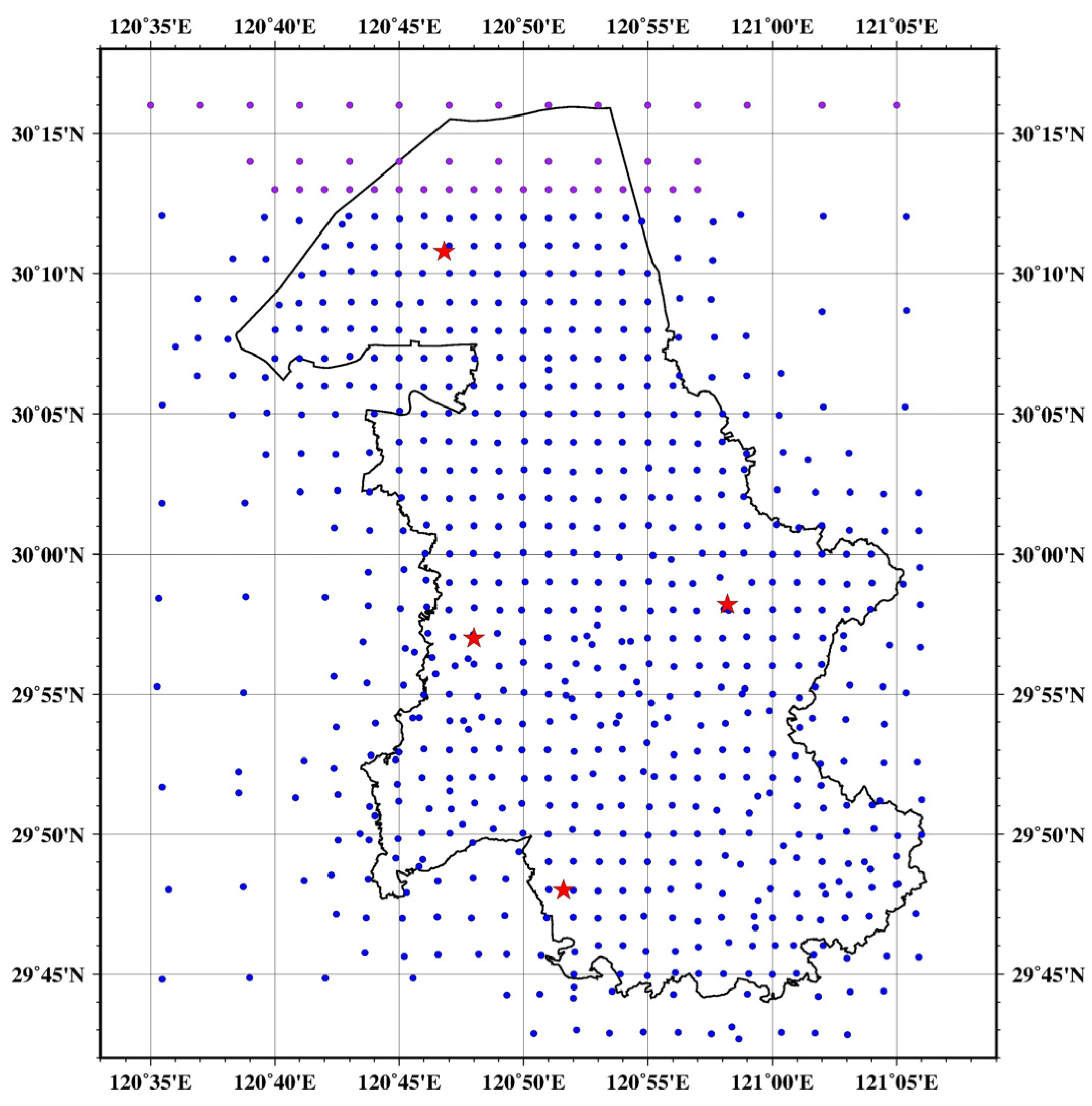
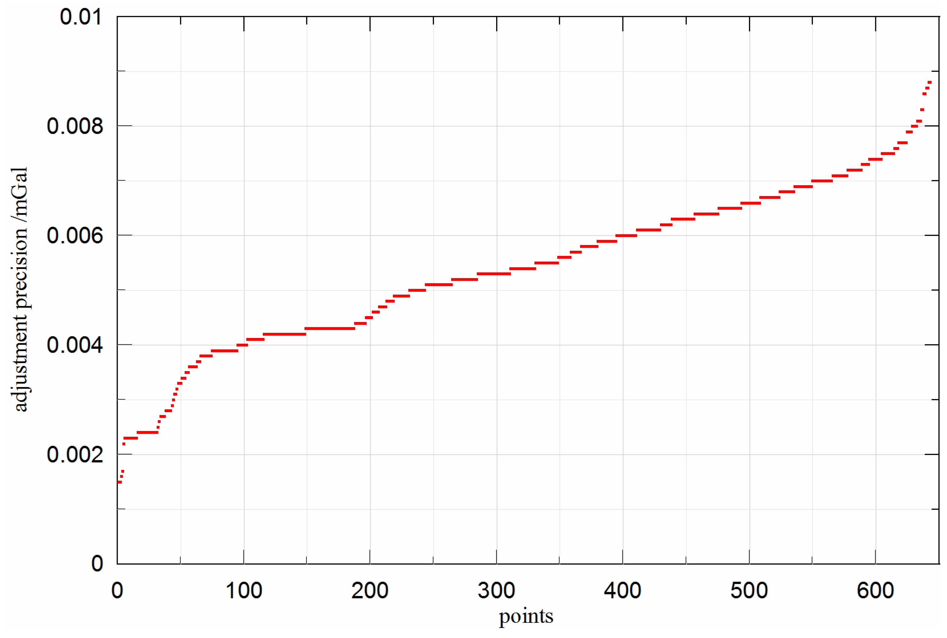
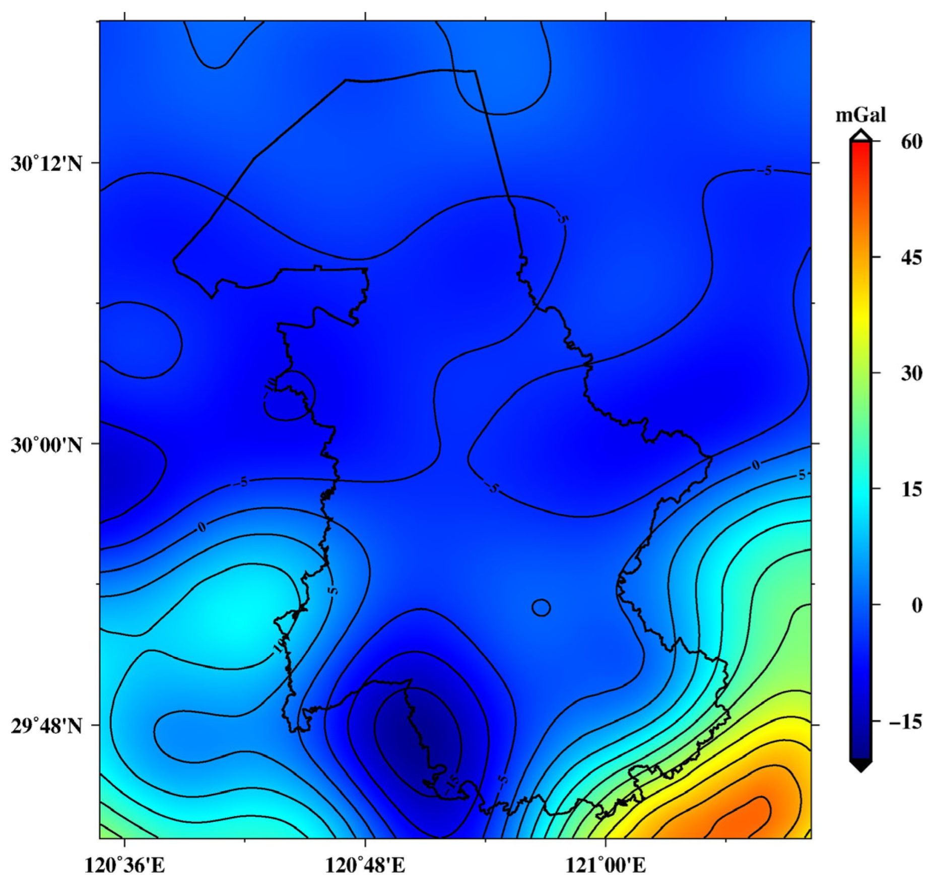
2.2. Ground Gravity Anomaly

Within the survey area, four gravity control-points were evenly distributed, and gravity observations were carried out employing a high-accuracy FG5X absolute gravimeter [24], adhering rigorously to the protocols specified in the “Specifications for the gravimetry control (GB/T 20256-2019)” [25]. The distributions of the gravity control-points are depicted in Figure 2 and denoted by red stars. The measured accuracy at each control point was better than 2 × 10⁻³ mGal (1 mGal = 10−5 m∙s−2).
Utilizing these gravity control-points, a comprehensive dataset comprising 643 terrestrial gravity measurements was obtained using the Scintrex CG-6 relative gravimeter [26], adhering to the protocols specified in the “Specifications for the dense gravity measurement (GB/T 17944-2018)” [27]. The distributions of the terrestrial gravity measurements are depicted in Figure 2 and denoted by blue dots. These measurements, characterized by a spatial resolution of 1.8 km within the Shangyu area, were tied to the National Gravity Fundamental Network 2000. The STD of the observational discrepancy, obtained from repeated observations at 10% of the points, is 4.7 × 10⁻³ mGal.
Then, the terrestrial gravity observational data undergo various preprocessing procedures, including corrections for solid tides, atmospheric pressure, tidal loading, instrument height, and zero drift, resulting in the gravity segment differences [28,29,30]. Subsequently, the classical LS adjustment method is executed combined with the control gravity data. The observational equations for the terrestrial gravity and the control point are formulated as follows [31]:
v i j = ( g ¯ j g ¯ i ) E × L i j v h = g ¯ h G h
where g ¯ i and g ¯ j represent the unknown gravity values at points i and j, respectively; L i j is the preprocessed value of the gravity segment difference between any two points i and j; E is the gravity instrument scale factor; g ¯ h is the unknown gravity value at the gravity control-point; G h is the observed gravity value at the control point; and v ij and v h are the adjustment corrections after the adjustment.
Equation (2) can be expressed as follows:
V = B X L ,   P g = σ 0 , gra 2 L 1
where V represents the correction vector [32], B is the coefficient matrix, X is the vector of unknowns, L is the vector of the observed values [33], and P g is a diagonal weight matrix that can be obtained using the a priori unit weight variance, σ 0 , gra 2 , and the known covariance matrix of the observations, L [34].
According to the LS criterion, the formula for solving the unknowns of gravity values is as follows:
X ^ = B T P g B 1 B T P g L Q X X = σ ^ 0 , gra 2 B T P g B 1 σ ^ 0 , gra 2 = V T P g V r
where X ^ is the matrix of the unknown gravity values to be determined, Q X X is the covariance matrix, σ ^ 0 , gra 2 is the variance of the unit weight, and r represents the degrees of freedom.
Figure 3 presents the statistical results of the adjustment precision, represented by σ ^ 0 , gra , as calculated in Equation (4), arranged in ascending order. The precision of the gravity values at all the measurement points averages 5.4 × 10⁻³ mGal. Next, the normal gravity field and free-air corrections are applied to the adjusted terrestrial gravity observations, yielding the free-air gravity anomaly.
Given the presence of the Qiantang River in the northernmost district of the Shangyu area, terrestrial measurements were impracticable. To overcome this limitation, we employed the latest release of the grav_32.1 model to supplement the missing data, ensuring their resolution matched those of the terrestrial measurements. The grav_32.1 model, obtained from the website https://topex.ucsd.edu/pub/global_grav_1min, accessed on 3 December 2022, incorporates an additional 12 months of data from Altika, Cryosat LRM, Cryosat SAR, and Sentinel-3A/B compared to previous versions. The grav_32.1 data used are represented by the purple dots in Figure, with maximum, minimum, and STD values of 1.47 mGal, −3.28 mGal, and 1.20 mGal, respectively.
Finally, the discrete free-air gravity anomaly underwent a gridding process to enhance its suitability for analysis, employing a fast Fourier-transform method in a series of steps. First, the topographic effects were removed through the application of the terrain and Bouguer correction to the free-air anomaly, resulting in the Bouguer anomaly, using a FORTRAN code—FA2BOUG [35]. Subsequently, interpolation onto a grid was executed, employing Shepard’s surface-fitting method [36]. This technique, widely recognized for its simplicity and straightforward implementation, entails the computation of weighted averages from known data points to estimate values at uncharted locations. Lastly, the topographic effect was reintegrated into the gridded Bouguer gravity anomalies. The maximum, minimum, mean, and STD values of the gridded free-air gravity anomaly were 61.26 mGal, −12.43 mGal, 4.38 mGal, and 11.02 mGal, respectively, as presented in Table 1.

2.3. GGM

Reference gravity anomalies were calculated based on a GGM. To select the optimal GGM, a criterion was established, aiming for a minimal STD of the difference between the terrestrial and reference gravity data. In this study, the Earth Gravitational Model EGM2008 [37], complete up to degree 2190 and order 2159, was utilized. A gravity anomaly grid, depicted in Figure 4, was generated using the services offered by the International Center for Global Earth Models (ICGEM) (http://icgem.gfz-potsdam.de, accessed on 15 August 2022). Following the recommendations of Sánchez et al. [38], reference gravity anomalies were determined in the tide-free system. In the tide-free system, the permanent deformation is eliminated from the geometric shape of the Earth. The gravity anomalies from EGM2008 are summarized in Table 1. The average reference gravity anomaly within the survey area is 0.99 mGal.
The degree error and cumulative degree error [39] play important roles as fundamental reference parameters for statistically analyzing and characterizing the spectral sensitivity of Earth’s gravitational field. In Figure 5a, the EGM2008 model exhibits its most significant degree errors at degree 108, followed by a gradual reduction.
Figure 5b illustrates the cumulative degree errors of the GGM. The cumulative degree variations in the EGM2008 model show a trend toward stabilization after reaching approximately 300, with minimal fluctuations observed.
Figure 6 displays the statistical outcomes concerning the disparity between the terrestrial gravity anomalies and the reference values. The discrepancies exhibit a normal distribution, and an assessment of the STD of discrepancies between the reference and free-air gravity anomalies yields a value of 8.4 mGal.

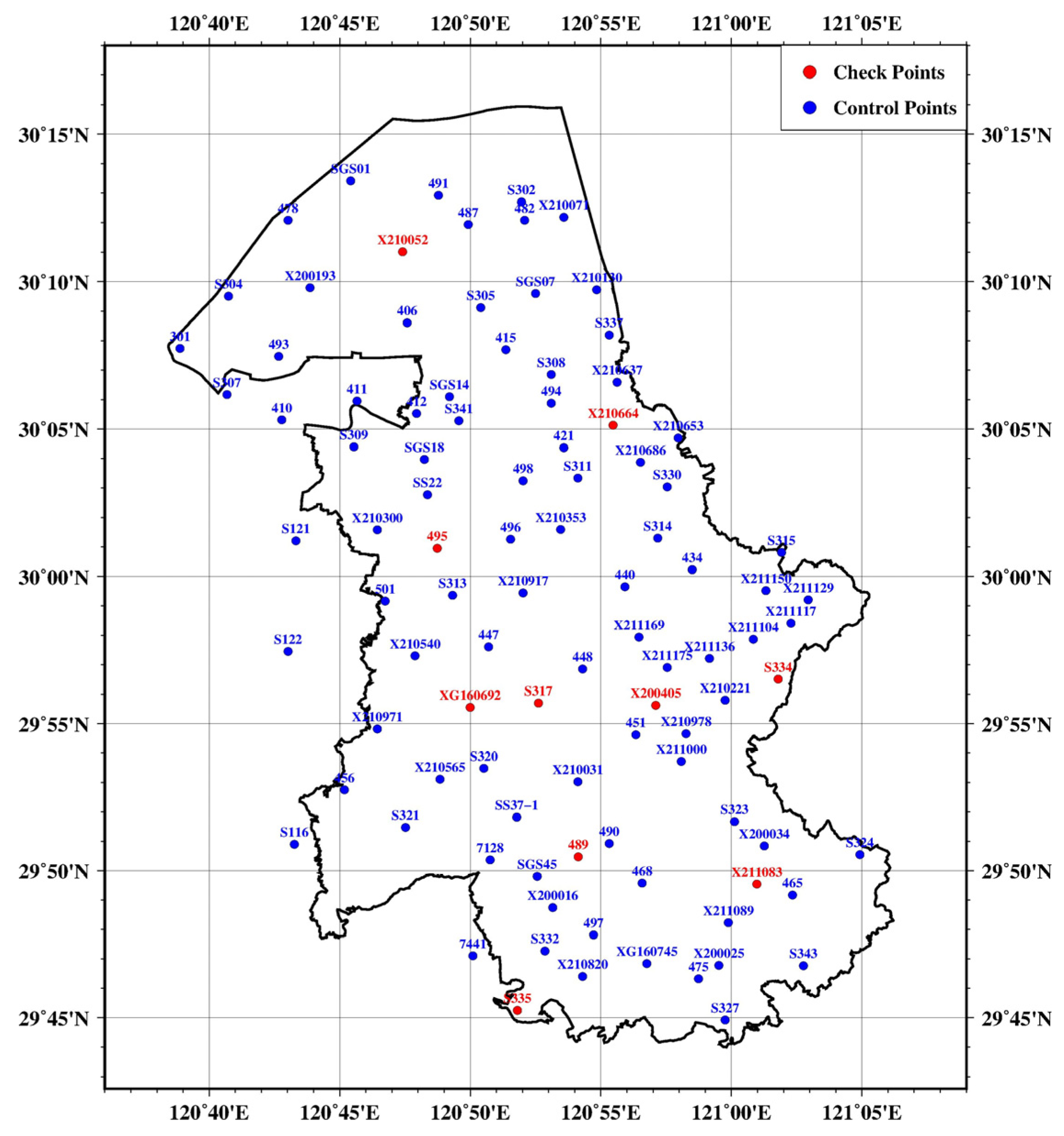
2.4. GNSS/Leveling Data

A total of 99 GNSS/leveling stations, evenly distributed within the study area, were utilized. Among them, 89 well-distributed GNSS benchmarks, indicated as blue dots in Figure 7, were treated as control points. These benchmark heights were subsequently integrated into the gravimetric quasi-geoid model, facilitating the development of a hybrid quasi-geoid model. Furthermore, 10 GNSS benchmarks, indicated as red dots in Figure 7, were used as check points to assess the accuracy and reliability of the hybrid quasi-geoid model.
The ellipsoidal heights at these benchmarks were referenced to the China Geodetic Coordinate System 2000 (CGCS2000), while the normal heights were referenced to the National Height Datum 1985, as determined through precise geometric leveling. According to the accuracy provided by the data provider, the mean square error (MSE) of the leveling measurements was determined to be ±0.56 mm per kilometer. In terms of repeatability, the baseline components of the GNSS network exhibited the following accuracies: 1.73 mm + 0.12 × 10⁻⁸·d in the north–south direction, 2.35 mm + 0.09 × 10⁻⁸·d in the east–west direction and better than 4.67 mm + 0.16 × 10⁻⁸·d in the vertical direction. For the baseline length direction, the accuracy was found to be 1.10 mm + 0.06 × 10⁻⁸·d, where d represents the distance between adjacent points.
Following a three-dimensional constrained adjustment, the relative planimetric accuracy of the GNSS network was determined to be 0.0011 ppm. The weakest edge of the network exhibited a relative accuracy of 0.0109 ppm, with a length of 42,738.0307 m. The weakest point within the GNSS network demonstrated a horizontal accuracy of 0.0031 m and a geodetic height accuracy of 0.0050 m.
The statistical assessment of the deviation between the ellipsoidal and leveling heights, denoted as GNSS/leveling heights, is summarized in Table 1. The average disparity is recorded as 10.72 m.

3. Method for Local Quasi-Geoid Determinations

3.1. Linearized Molodensky’s Solution

Molodensky’s problem has been approached using various methods in practical calculations [12,14]. In this study, a rigorous formulation for the Molodensky series terms was employed.
The boundary value problem of Molodensky is represented mathematically as [40]
T r + 2 r T Σ = Δ g
where ∆g is the gravity anomaly, and T is the disturbing potential [13],
T = Σ φ l d Σ
where φ represents the density of the masses of a single layer at the physical surface [41], Σ denotes the telluroid surface, and l is the distance from point P to the telluroid element, d Σ ,
l = r P 2 + r 2 2 r P r cos ψ
where r = R + h; rp = R + hp; and hp is the normal height of the computation point, P; h denotes the normal height of the running point; R is the average radius of the Earth; and ψ is the spherical distance between the computation point and the integration element.
Taking into account the discontinuity of the derivative of the gravitational potential [42], then we have
T r P = 2 π φ cos β + Σ φ r P 1 l d Σ
The slope of the telluroid, β, is the angle between the normal of Earth’s surface and the radial direction.
By substituting Equation (8) into the boundary condition presented in Equation (5) and considering that d Σ cos β = r 2 d σ , where σ is the unit sphere, Δ g can be expressed as follows:
Δ g = 2 π φ cos β σ 3 2 l + r 2 r P 2 2 l 3 r 2 r P sec β φ d σ
By letting θ = φ sec β , Equation (9) can be written as follows:
Δ g = 2 π θ 1 + tan 2 β 1 σ 3 R 2 l + R 2 h h P l 3 θ d σ
By introducing a factor k ∈ [0, 1] [43], the function θ is expanded into a series of k ,
θ = n = 0 k 2 θ n
And for this equation to hold, all the coefficients of the same power of k must be zero. Molodensky’s integral equation is written as
2 π θ n 3 2 R σ θ n l 0 d σ = G n
where l 0 = 2 R sin ψ 2 [44].
G n can be obtained,
G 0 = Δ g G 1 = R 2 σ h h P l 0 3 θ 0 d σ G 2 = R 2 σ h h P l 0 3 θ 1 d σ     3 R 4 σ h h P 2 l 0 3 θ 0 d σ + 2 π θ 0 tan 2 β
Let
R 2 σ θ n l 0 d σ = T n
By combining Equations (12) and (14), T n can be computed as follows:
T n = R 4 π σ G n S ψ d σ
where S(ψ) corresponds to the spherical Stokes’ function with the argument ψ, and θ n is expressed as follows:
θ n = 1 2 π G n + 3 2 R T n = 1 2 π G n + 3 16 π 2 σ G n S ψ d σ
Extending this methodology allows us to sequentially solve for θ n and G n . Throughout this process, T n can be computed as follows [45]:
T 0 = R 4 π σ G 0 S ψ d σ T 1 = R 4 π σ G 1 S ψ d σ T 2 = R 4 π σ G 2 S ψ d σ R 2 2 σ h h p 2 l 0 3 θ 0 d σ
The computation of T 0 involved the utilization of Stokes’ integral, revealing the connections and differences between Molodensky’s and Stokes’ theories [2]. The inclusion of higher-order terms (for n ≥ 1) in the analysis accounts for the influence of the topographic undulation surrounding the computation point.
The height anomaly at the ground station can be obtained according to Bruns’ formula [46] as follows:
ζ n = T n γ
where γ is normal gravity.
The solution for the gravimetric quasi-geoid is given by the following formally identical infinite series:
ζ grav = n = 0 ζ n

3.2. Combination of Heights

The fundamental concept behind the multi-surface function [47] entails approximating a continuous regular or irregular surface using a small number of simple surfaces. This approach involves constructing a surface for each data point and subsequently merging these surfaces to form a seamless, continuous whole surface, while ensuring strict alignment with each individual data point. From a geometric perspective, the multi-surface function serves as an exceptional interpolation method that effectively addresses the challenge for adjusting a mathematical surface based on data points.
If there are u well-distributed control benchmarks with known GNSS-derived ellipsoidal and leveling normal heights, the multi-surface function for estimating the quasi-geoid height can be formulated as follows:
ζ ϕ , λ = ζ grav ϕ , λ + j = 1 m a j ϕ ϕ j 2 + λ λ j 2
were ζ grav ϕ , λ represents the gravimetric quasi-geoid model, ϕ , λ denotes the coordinates of the interpolation points, ϕ j , λ j is coordinate of the known point, m is the number of known points, and aj is the parameter to be determined. The resulting quasi-geoid height is denoted by ζ ϕ , λ .
The determination of the unknown model parameters is carried out using the LS method [48]. We consider the following linear functional model:
v = A x w
where v is the error vector, A is the coefficient matrix of the multi-surface function, x is the unknown parameter vector of the multi-surface function model, and w is the following observation vector:
w = h 1 H 1 ζ 1 grav h u H u ζ u grav = w 1 w u
where h i is the known GNSS-derived ellipsoidal height, and H i is the known leveling normal height.
The unknown parameters and the adjusted residuals can be expressed as
x ^ = A T P A 1 A T P w
v ^ = A x ^ w
where x ^ is the parameter vector, v ^ is the adjusted error vector, and P is a weight matrix of the observation, which is determined based on the a priori statistical behavior of errors, v ,
P = 1 σ 0 2 E v v 1
where σ 0 2 is the unit weight variance.
The availability of covariance matrices for GNSS ellipsoidal and normal heights is not always straightforward. Hence, to account for the influence of the distance on the data points, initial weights are typically assigned based on their horizontal distances [49] from the interpolation point as follows:
P i j = 0 ,   for   i j P i i = C 0 2 D i + ε 2 , i = 1 , 2 , , n
where C 0 represents the unit weight length, D i is the horizontal distance between the observation and interpolation points, and ε is an arbitrary constant commonly set to ε = 0.01 in practical applications.
The initial weight computed using Equation (26) assumes the reliability of all the values. However, data points often contain outliers due to observation errors and although the LS method can account for errors, it is unable to effectively handle interference from gross errors or outliers. To mitigate the influence of abnormal data points, a robust estimation technique is introduced to estimate the model parameters. A practical approach involves employing the following iterative solution formula:
x ^ q = A T P q A 1 A T P q w
where q represents the number of iterative steps, and P q is the equivalent weight, which can be obtained by iterative computing as follows [50]:
P i q + 1 = P i q for   T i < C P i q exp T i C for   T i C
where
T i = v ^ i P i σ ^ 0
where C is a constant typically set to C = 3 .

4. Results and Discussion

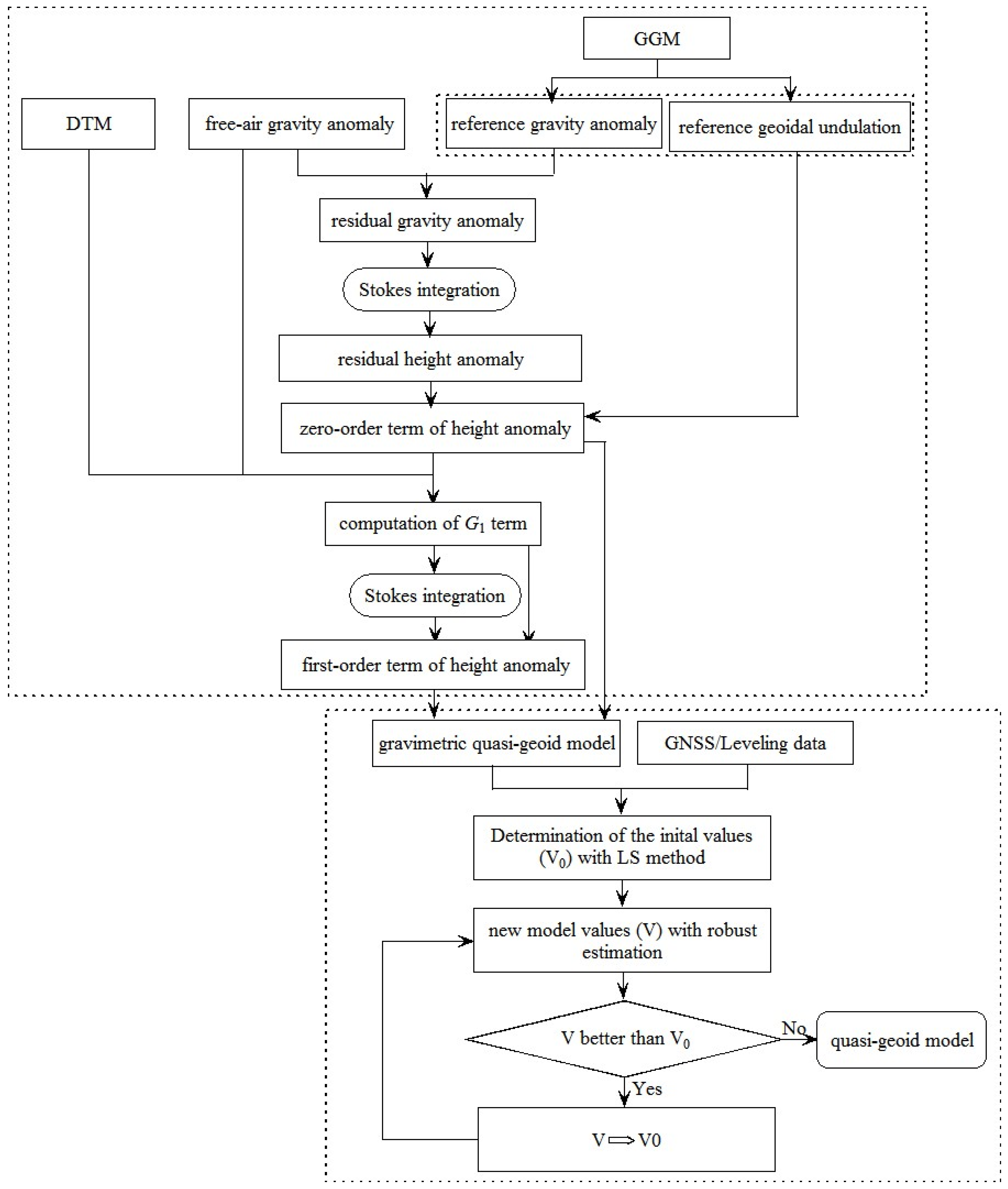
4.1. Computation of Hybrid Quasi-Geoid Model

The determination of the quasi-geoid model over the Shangyu area involved two main steps: the computation of the gravimetric quasi-geoid model and the integration of heterogeneous heights. The computational procedures for quasi-geoid determination are depicted in Figure 8.
In the first step, Molodensky’s BVP theory was applied to construct the gravimetric quasi-geoid model. Considering that the impact of the G2 term on the height anomaly within the test area was found to be negligible, measuring less than 1 mm, the contributions of the G2 term as well as the higher-order terms were disregarded. The computational procedure adopted for the gravimetric quasi-geoid model was as follows:
  • Computation of the zero-order term of the height anomaly: The residual height anomaly was computed using Stokes’ theory by taking the difference (residual gravity anomaly) between the free-air and reference gravity anomalies derived from EGM2008. Adding the reference geoidal undulation to the residual height anomaly yielded the zero-order term of the height anomaly, ζ0;
  • Computation of the G1 term: Utilizing Equation (13), the G1 term was determined based on the DTM, the gridded free-air anomaly, and the zero-order term of the height anomaly, ζ0;
  • Computation of the first-order term of the height anomaly: The effect of the first-order term on height anomaly, denoted as ζ1, was obtained using the spherical Stokes’ integral given by
ζ 1 = R 4 π γ σ G 1 S ψ d σ
The contributions of the G1 term to both the gravity and height anomalies are illustrated in Figure 9a,b, respectively. In particular, the effect of the G1 term on the height anomalies exhibited a maximum value of 1.2 cm in the southeastern part of the study area. This outcome aligns with expectations as this region experiences higher and more variable topographic heights. However, in the northern region, where the terrain is relatively lower and smoother, the effect of the G1 term was comparatively small.
4.
Computation of the gravimetric quasi-geoid model: The gravimetric quasi-geoid model, denoted as ζgrav is expressed by
ζ grav = ζ 0 + ζ 1
The calculated gravimetric quasi-geoid model covered a geographical area ranging from 29.72°N to 30.3°N latitude and from 120.58°E to 121.2°E longitude, with a grid spacing of 1′ × 1′. The STD of the differences between the GNSS/leveling heights and the gravimetric quasi-geoid model was found to be 1.8 cm.
In the second step, we employed a multi-surface function of LS based on GNSS benchmarks with a known gravimetric quasi-geoid, normal heights, and ellipsoidal heights to interpolate the hybrid quasi-geoid heights. To reduce the potential influence of abnormal data points, a robust estimation technique was implemented. The following procedure was adopted to create the hybrid quasi-geoid: (1) Computation of height differences: We computed the differences between the observed GNSS/leveling heights and the gravimetric quasi-geoid heights. (2) Construction of a correction grid: Using the multi-surface function and robust estimation, we constructed a 1′ × 1′ grid from the height differences, referred to as the “correction” grid. (3) Addition of the geoid correction: The geoid “correction” grid was added to the grid of the gravimetric quasi-geoid, resulting in the hybrid quasi-geoid model on a 1′ × 1′ grid.
The statistical results regarding the differences between the hybrid quasi-geoid and the reference geoidal undulation from EGM2008 as well as the differences between the hybrid quasi-geoid and the gravimetric quasi-geoid, after removing the systematic bias, are presented in Table 2. According to the table, the STD of the differences between the hybrid quasi-geoid and the reference geoidal undulation from EGM2008 is 4.9 cm, whereas the STD of the differences between the hybrid quasi-geoid and the gravimetric quasi-geoid is 1.8 cm.

4.2. Accuracy Assessment

To evaluate the accuracy of the hybrid quasi-geoid over the Shangyu area, we utilized interpolation techniques to determine quasi-geoid undulations at the coordinates of each GNSS/leveling station. Subsequently, a thorough accuracy assessment was conducted.
First, the accuracy was established by comparing the hybrid quasi-geoid model with the observed GNSS/leveling heights at the 89 control points, as depicted in Figure 10a. The analysis revealed that the maximum, minimum, and STD values of the differences between the hybrid quasi-geoid model with the GNSS/leveling heights at the control points are 0.85 cm, −0.74 cm, and 0.21 cm, respectively.
To further assess the accuracy, a comparison was made between the hybrid quasi-geoid heights and the height anomaly derived from GNSS/leveling surveys at 10 independent check points, as illustrated in Figure 10b. The maximum, minimum, and STD values of the differences between these measurements were calculated to be 1.24 cm, −1.66 cm, and 0.79 cm, respectively.
These results provide a comprehensive evaluation of the accuracy of the hybrid quasi-geoid model, demonstrating its accuracy in estimating quasi-geoid heights. The small differences between the model and the observed heights indicate its reliability for various applications, such as geodetic surveys, engineering projects, and geophysical studies.

5. Conclusions

In this study, we have adopted an integrated approach to analyze ellipsoidal and normal heights together with a gravimetric quasi-geoid, with the objective of constructing a hybrid quasi-geoid model with millimeter-level accuracy over the Shangyu area. To achieve this, we optimized the utilization of various data sources, including terrestrial gravity measurements, a GGM, GNSS/leveling heights, and DTM data.
Our approach is based on Molodensky’s theory and encompasses a comprehensive framework that provides rigorous and practical formulae for Molodensky’s series solution. This series solution incorporates the non-level nature of the Earth’s surface and enables precise modeling of the quasi-geoid, particularly in regions characterized by significant topographic variations. The STD of the differences between the gravimetric quasi-geoid and GNSS/leveling heights was determined to be 1.8 cm, indicating satisfactory overall agreement between these measurements.
Subsequently, we employed the multi-surface function combined with LS techniques to interpolate hybrid quasi-geoid heights, using ellipsoidal and normal heights as well as gravimetric quasi-geoid data. Because the measurements may contain significant errors and the interpolation approach had some limitations, traditional LS estimation did not yield optimal results for these smaller datasets. Robust analysis methods, however, work well. To mitigate the influence of outliers, we introduced a robust technique for estimating the model parameters. This ensured the robustness and reliability of the interpolation process. By applying the proposed procedure, the accuracy of the hybrid quasi-geoid model with GNSS/leveling heights at 89 control points reached 0.21 cm. Furthermore, the accuracy determined by evaluating the absolute agreement between the hybrid quasi-geoid model and GNSS/leveling heights at 10 independent check points, demonstrated satisfactory results, with an accuracy of 0.79 cm.
Overall, our study presents a unified and optimized approach that integrates various data sources and utilizes advanced modeling techniques to generate a highly accurate hybrid quasi-geoid model for the Shangyu area.

Author Contributions

Conceptualization, D.G.; methodology, D.G., X.C. and Z.X.; validation, D.G. and Z.X.; formal analysis, D.G., H.H. and L.X.; software, D.G. and X.N.; investigation, D.G. and X.M.; resources, D.G., L.X. and X.N.; data curation, X.C., L.X., X.M. and X.N.; writing—original draft preparation, D.G.; writing—review and editing, D.G., X.C., Z.X., H.H., L.X., X.M. and X.N.; visualization, D.G., Z.X., H.H. and X.M.; supervision, D.G.; funding acquisition, D.G. and X.C.; project administration, D.G. and X.C. All authors have read and agreed to the published version of the manuscript.

Funding

This work was funded by the Basic Frontier Science Research Program of the Chinese Academy of Sciences (No. ZDBS-LY-DQC028).

Data Availability Statement

The SRTM3 data underlying this article are available at https://srtm.csi.cgiar.org/srtmdata, accessed on 20 August 2022, EGM2008 is available at http://icgem.gfz-potsdam.de/tom_longtime, accessed on 15 August 2022, and the grav_32.1 model is available at https://topex.ucsd.edu/pub/global_grav_1min/, accessed on 3 December 2022.

Acknowledgments

We extend our thanks to the International Centre for Global Earth Models (ICGEMs) and the NASA Shuttle Radar Topographic Mission (SRTM) for their kind provision of the global geopotential models and the digital terrain model data, respectively. The authors are sincerely appreciative of the diligent efforts of the anonymous reviewers, whose contributions significantly improved the quality of this work.

Conflicts of Interest

The authors declare no conflict of interest.

References

  1. Brennecke, J.; Groten, E. The deviations of the sea surface from the geoid and their effect on geoid computation. Bull. Geod. 1977, 51, 47–51. [Google Scholar] [CrossRef]
  2. Sansò, F.; Sideris, M.G. Geoid Determination: Theory and Methods, Lecture Notes in Earth System Sciences; Springer: Berlin/Heidelberg, Germany, 2013. [Google Scholar]
  3. Steinbergerk, B.; Rathnayake, S.; Kendall, E. The Indian Ocean Geoid Low at a plume-slab. Tectonophysics 2021, 817, 229037. [Google Scholar] [CrossRef]
  4. Falcão, A.P.; Matos, J.; Gonçalves, A.; Casaca, J.; Sousa, J. Preliminary Results of Spatial Modelling of GPS/Levelling Heights: A Local Quasi-Geoid/Geoid for the Lisbon Area. In Gravity, Geoid and Earth Observation; International Association of Geodesy, Symposia; Mertikas, S., Ed.; Springer: Berlin/Heidelberg, Germany, 2010; Volume 135. [Google Scholar]
  5. Fotopoulos, G. Calibration of geoid error models via a combined adjustment of ellipsoidal, orthometric and gravimetric geoid height data. J. Geod. 2005, 79, 111–123. [Google Scholar] [CrossRef]
  6. Grigoriadis, V.N.; Vergos, G.S.; Barzaghi, R.; Carrion, D.; Koc, O. Collocation and FFT-based geoid estimation within the Colorado 1 cm geoid experiment. J. Geod. 2021, 95, 52. [Google Scholar] [CrossRef]
  7. Sansò, F.; Rummel, R. Geodetic Boundary Value Problems in View of the One Centimeter Geoid; Springer: Berlin/Heidelberg, Germany, 1977. [Google Scholar]
  8. Kotsakis, C.; Tsalis, I. Combination of Geometric and Orthometric Heights in the Presence of Geoid and Quasi-geoid Models. In Gravity, Geoid and Height Systems; International Association of Geodesy, Symposia; Marti, U., Ed.; Springer: Cham, Switzerland, 2014; Volume 141. [Google Scholar]
  9. Featherstone, W.E.; Olliver, J.G. A method to validate gravimetric-geoid computation software based on Stokes’s integral formula. J. Geod. 1997, 71, 571–576. [Google Scholar] [CrossRef]
  10. Sjöberg, L.E. Topographic effects by the Stokes-Helmert method of geoid and quasi-geoid determinations. J. Geod. 2000, 74, 255–268. [Google Scholar] [CrossRef]
  11. Ardestani, V.E.; Martinec, Z. Geoid determination through ellipsoidal Stokes boundary-value problem. Stud. Geophys. Et Geod. 2000, 4, 353–363. [Google Scholar] [CrossRef]
  12. Molodensky, M.S.; Eremeev, V.F.; Yurkina, M.I. Methods for the Study of the External Gravitational Field and Figure of the Earth; Israeli Program for Scientific Translations: Jerusalem, Israel, 1962. [Google Scholar]
  13. Brovar, V.V. On the solution of Molodensky’s boundary value problem. Bull. Geod. 1964, 72, 167–173. [Google Scholar] [CrossRef]
  14. Ardalan, A.A.; Grafarend, E.W.; Ihde, J. Molodensky potential telluroid based on a minimum-distance map. Case study: The quasi-geoid of East Germany in the World Geodetic Datum 2000. J. Geod. 2002, 76, 127–138. [Google Scholar] [CrossRef]
  15. Kuroishi, Y.; Ando, H.; Fukuda, Y. A new hybrid geoid model for Japan, GSIGE02000. J. Geod. 2002, 76, 428–436. [Google Scholar] [CrossRef]
  16. Nahavandchi, H.; Soltanpour, A. Improved determination of heights using a conversion surface by combining gravimetric quasi-geoid/geoid and GPS-levelling height differences. Stud. Geophys. Geod. 2006, 50, 165–180. [Google Scholar] [CrossRef]
  17. Tziavos, I.N.; Vergos, G.S.; Grigoriadis, V.N.; Andritsanos, V.D. Adjustment of Collocated GPS, Geoid and Orthometric Height Observations in Greece. Geoid or Orthometric Height Improvement? In Geodesy for Planet Earth; International Association of Geodesy, Symposia; Kenyon, S., Pacino, M., Marti, U., Eds.; Springer: Berlin/Heidelberg, Germany, 2012; Volume 136. [Google Scholar]
  18. Hwang, C.; Hsu, H.; Featherstone, W.; Cheng, C.; Yang, M.; Huang, W.; Wang, C.; Huang, J.; Chen, K.; Huang, C.; et al. New gravimetric-only and hybrid geoid models of Taiwan for height modernisation, cross-island datum connection and airborne LiDAR mapping. J. Geod. 2020, 94, 83. [Google Scholar] [CrossRef]
  19. Yang, Y. Robust estimation of geodetic datum transformation. J. Geod. 1999, 73, 268–274. [Google Scholar] [CrossRef]
  20. Awange, J.L.; Paláncz, B. Robust Estimation. In Geospatial Algebraic Computations; Springer: Cham, Switzerland, 2016. [Google Scholar]
  21. Denker, H. Evaluation of SRTM3 and GTOPO30 terrain data in Germany. In International Association of Geodesy Symposia; Springer: Cham, Switzerland, 2005; Volume 129, pp. 218–223. [Google Scholar]
  22. Amante, C.; Eakins, B.W. ETOPO1, 1 Arc-Minute Global Relief Model: Procedures, Data Sources and Analysis; NOAA Technical Memorandum NESDIS; National Geophysical Data Center, NOAA: Boulder, CO, USA, 2000; Volume 24, p. 19.
  23. Yang, M.; Hirt, C.; Rexer, M.; Pail, R.; Yamazaki, D. The tree canopy effect in gravity forward modelling. Geophys. J. Int. 2019, 219, 271–289. [Google Scholar] [CrossRef]
  24. Scherneck, H.G.; Rajner, M.; Engfeldt, A. Superconducting gravimeter and seismometer shedding light on FG5’s offsets, trends and noise: What observations at Onsala Space Observatory can tell us. J. Geod. 2020, 94, 80. [Google Scholar] [CrossRef]
  25. GB/T 20256-2019; Specifications for the Gravimetry Control. Standards Press of China: Beijing, China, 2019.
  26. Francis, O. Correction to: Performance assessment of the relative gravimeter Scintrex CG-6. J. Geod. 2022, 96, 2. [Google Scholar] [CrossRef]
  27. GB/T 17944-2018; Specifications for the Dense Gravity Measurement. Standards Press of China: Beijing, China, 2019.
  28. Dziewonski, A.M.; Anderson, D.L. Preliminary reference earth model. Phys. Earth Planet. Inter. 1981, 25, 297–356. [Google Scholar] [CrossRef]
  29. Merriam, J.B. Atmospheric pressure and gravity. Geophys. J. Int. 1992, 190, 488–500. [Google Scholar] [CrossRef]
  30. Spratt, R.S. Modelling the effect of atmospheric pressure variations on gravity. Geophys. J. R. Astron. Soc. 1982, 71, 173–186. [Google Scholar] [CrossRef]
  31. Wei, S.C.; Xu, J.Q.; Zhou, J.C. Piece-wise linear dynamic adjustment for gravity network. Acta Geod. Cartogr. Sin. 2016, 45, 511–520. [Google Scholar]
  32. Wijaya, D.D.; Muhammad, N.A.; Prijatna, K.; Sadarviana, V.; Sarsito, D.A.; Pahlevi, A.; Variandy, E.D.; Putra, W. pyGABEUR-ITB: A free software for adjustment of relative gravimeter data. Geomatika 2019, 25, 95–102. [Google Scholar] [CrossRef]
  33. Hwang, C.; Wang, C.G.; Lee, L.H. Adjustment of relative gravity measurements using weighted and datum-free constraints. Comput. Geosci. 2002, 28, 1005–1015. [Google Scholar] [CrossRef]
  34. Lagios, E. A Fortran IV program for a least-squares gravity base-station network adjustment. Comput. Geosci. 1983, 10, 263–276. [Google Scholar] [CrossRef]
  35. Fullea, J.; Fernàndez, M.; Zeyen, H. FA2BOUG-A FORTRAN 90 code to compute Bouguer gravity anomalies from gridded free-air anomalies: Application to the Atlantic-Mediterranean transition zone. Comput. Geosci. 2008, 34, 1665–1681. [Google Scholar] [CrossRef]
  36. Shepard, D. A Two-Dimensional Interpolation Function for Irregularly Spaced Data. In Proceedings of the 23rd National Conference ACM, New York, NY, USA, 27–29 August 1968; pp. 517–523. [Google Scholar]
  37. Pavlis, N.K.; Holmes, S.A.; Kenyon, S.C.; Factor, J.K. An earth gravitational model degree 2160: EGM2008. In Proceedings of the 2008 General Assembly of the European Geosciences Union, Vienna, Austria, 13–18 April 2008. [Google Scholar]
  38. Sánchez, L.; Ågren, J.; Huang, J.; Wang, Y.M.; Forsberg, R. Basic Agreements for the Computation of Station Potential Values as IHRS Coordinates, Geoid Undulations and Height Anomalies within the Colorado 1 cm Geoid Experiment. In Proceedings of the International Symposium on Gravity, Geoid and Height Systems 2018 (GGHS2018), Copenhagen, Denmark, 17–21 September 2018. [Google Scholar]
  39. Pail, R.; Bruinsma, S.; Migliaccio, F.; Förste, C.; Goiginger, H.; Schuh, W.-D.; Höck, E.; Reguzzoni, M.; Brockmann, J.M.; Abrikosov, O.; et al. First GOCE gravity field models derived by three different approaches. J. Geod. 2011, 85, 819–843. [Google Scholar] [CrossRef]
  40. Vaľko, M.; Mojzeš, M.; Janák, J.; Papčo, J. Comparison of two different solutions to Molodensky’s G1 term. Stud. Geophys. Geod. 2008, 52, 71–86. [Google Scholar] [CrossRef]
  41. Tiron, M. Some problems regarding the way of solving Molodensky’s integral equation for the earth considered as a plane. Stud. Geophys. Et Geod. 1965, 9, 137–144. [Google Scholar] [CrossRef]
  42. Moritz, H. Series solutions of Molodensky’s problem. Publ. Deut. Geod. Komm. 1971, A, 70. [Google Scholar] [CrossRef]
  43. Guo, J.Y. Physical Geodesy. Springer Textbooks in Earth Sciences, Geography and Environment; Springer: Cham, Switzerland, 2023. [Google Scholar]
  44. Sideris, M.G.; Schwarz, K.P. Solving Molodensky’s series by fast Fourier transform techniques. Bull. Geod. 1986, 60, 51–63. [Google Scholar] [CrossRef]
  45. Müssle, M.; Heck, B.; Seitz, K.; Grombein, T. On the effect of planar approximation in the Geodetic Boundary Value Problem. Stud. Geophys. Geod. 2014, 58, 536–555. [Google Scholar] [CrossRef]
  46. Heiskanen, W.A.; Moritz, H. Physical Geodesy; Freeman: San Francisco, CA, USA, 1967. [Google Scholar]
  47. Yu, B.; Guan, Z.; Xu, X.; Yang, L.O. The Application of an Improved Multi-surface Function Based on Earth Gravity Field Model in GPS Leveling Fitting. In Geo-Informatics in Resource Management and Sustainable Ecosystem GRMSE; Communications in Computer and Information, Science; Bian, F., Xie, Y., Cui, X., Zeng, Y., Eds.; Springer: Berlin/Heidelberg, Germany, 2013; Volume 399. [Google Scholar]
  48. Klees, R.; Prutkin, I. The combination of GNSS-levelling data and gravimetric (quasi-) geoid heights in the presence of noise. J. Geod. 2010, 84, 731–749. [Google Scholar] [CrossRef]
  49. Watson, D.F.; Philip, G.M. A refinement of inverse distance weighted interpolation. Geo-Processing 1985, 2, 315–327. [Google Scholar]
  50. Kubik, K. An error theory for the Danish method. In Proceedings of the Symp Math Models, Accuracy Aspects and Quality Control, ISPRS Commission III Symposium, Helsinki, Finland, 7–11 June 1982. [Google Scholar]
Figure 1. Topographic data (black line is the administrative boundary of the Shangyu area).
Remotesensing 15 05414 g001
Figure 2. Gravity measurements (red stars indicate the gravity control-points, blue dots indicate the terrestrial gravity points, and purple dots indicate the grav_32.1).
Remotesensing 15 05414 g002
Figure 3. Statistical results of the adjustment precision for terrestrial gravity points.
Remotesensing 15 05414 g003
Figure 4. Reference gravity anomaly computed with EGM2008 model.
Remotesensing 15 05414 g004
Figure 5. (a) Degree error and (b) cumulative degree error of the GGM.
Remotesensing 15 05414 g005
Figure 6. Statistical results of the difference between the reference and terrestrial gravity anomalies.
Remotesensing 15 05414 g006
Figure 7. GNSS/Leveling stations (blue dots indicate the control points, and red dots indicate the check points).
Remotesensing 15 05414 g007
Figure 8. Flowchart of quasi-geoid determination.
Remotesensing 15 05414 g008
Figure 9. Contributions of Molodensky first-order term: (a) G1 values and (b) ζ1 values.
Remotesensing 15 05414 g009
Figure 10. (a) Differences between the hybrid quasi-geoid model and observed heights at the control points, and (b) differences between the hybrid quasi-geoid model and observed heights at the check points.
Remotesensing 15 05414 g010
Table 1. Statistics of the input data.
ModelMaxMinMeanSTD
GNSS/leveling heights (m)11.729.8210.720.44
topographic data (m)960.38−34.81108.80179.74
terrestrial gravity (mGal)61.26−12.434.3811.02
reference gravity anomalies (mGal)50.97−18.510.9911.93
Table 2. Comparisons of the hybrid quasi-geoid model with reference height anomaly from EGM2008 and gravimetric quasi-geoid (unit: m).
ModelMaxMinSTD
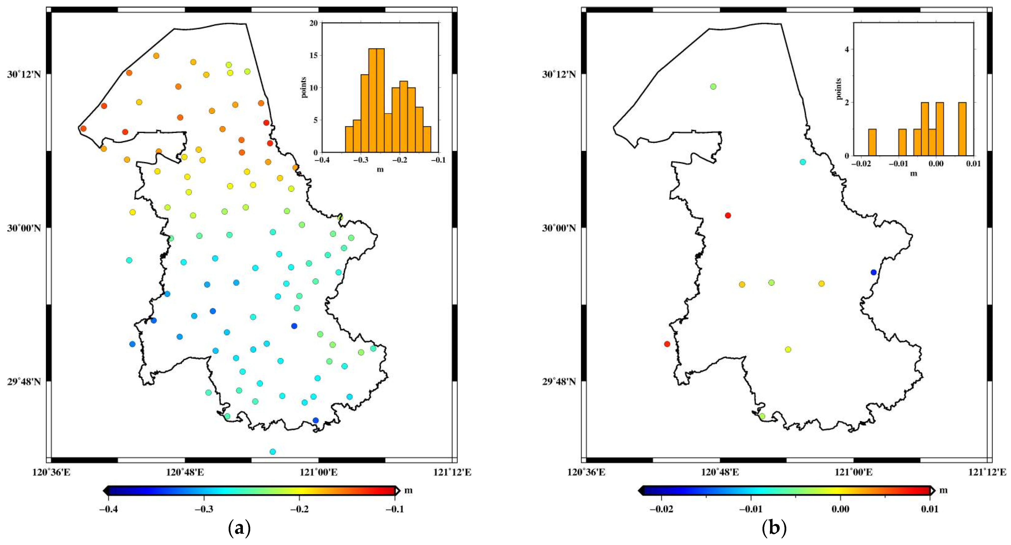
compared with reference height anomalies0.117−0.1110.049
compared with gravimetric quasi-geoid0.049−0.0350.018
Disclaimer/Publisher’s Note: The statements, opinions and data contained in all publications are solely those of the individual author(s) and contributor(s) and not of MDPI and/or the editor(s). MDPI and/or the editor(s) disclaim responsibility for any injury to people or property resulting from any ideas, methods, instructions or products referred to in the content.

