
Slope-Scale Evolution Categorization of Deep-Seated Slope Deformation Phenomena with Sentinel-1 Data
 ,
,  ,
,  ,
,  ,
,  ,
,  ,
,  ,
,  and
and 
Abstract
:
1. Introduction
2. Materials and Methods
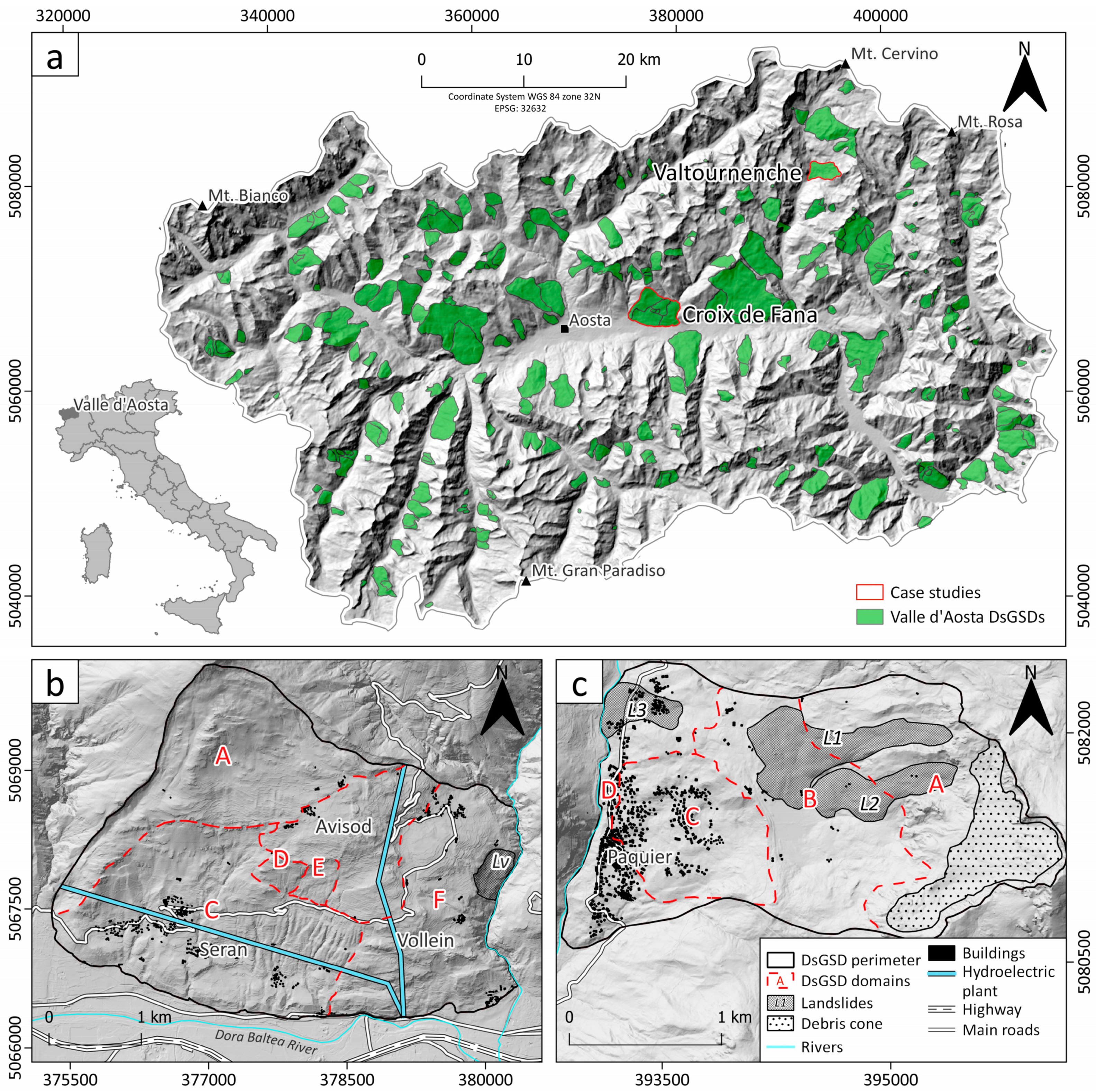
2.1. DsGSD Morpho-Structural Domains
2.2. Sentinel-1 Datasets and A-DInSAR Processing Methodology
2.3. SAR Data Coverage Analysis
2.4. SAR Data Suitability Analysis
2.5. SAR Data Interpolation
3. Results
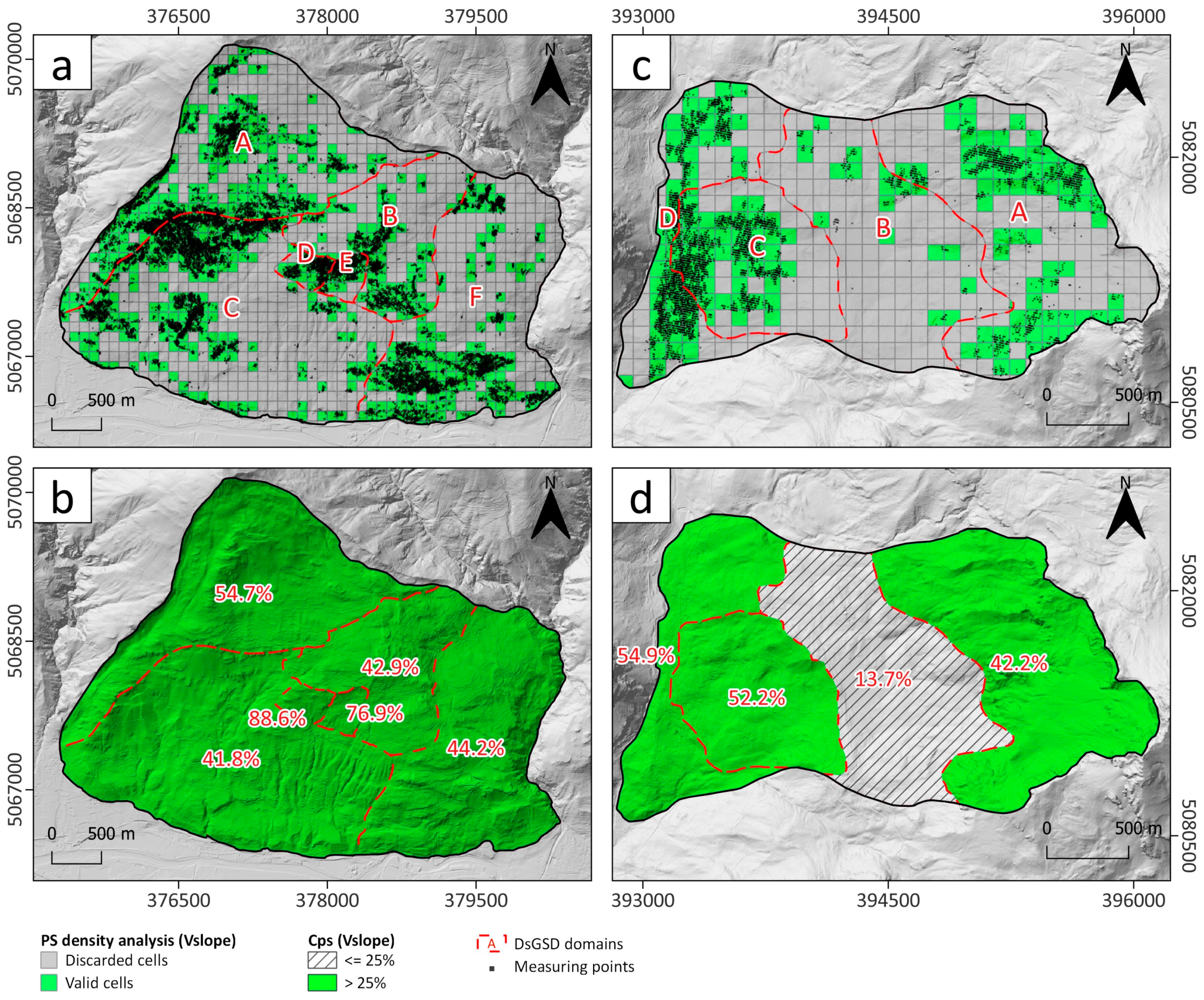
3.1. PS Density Map
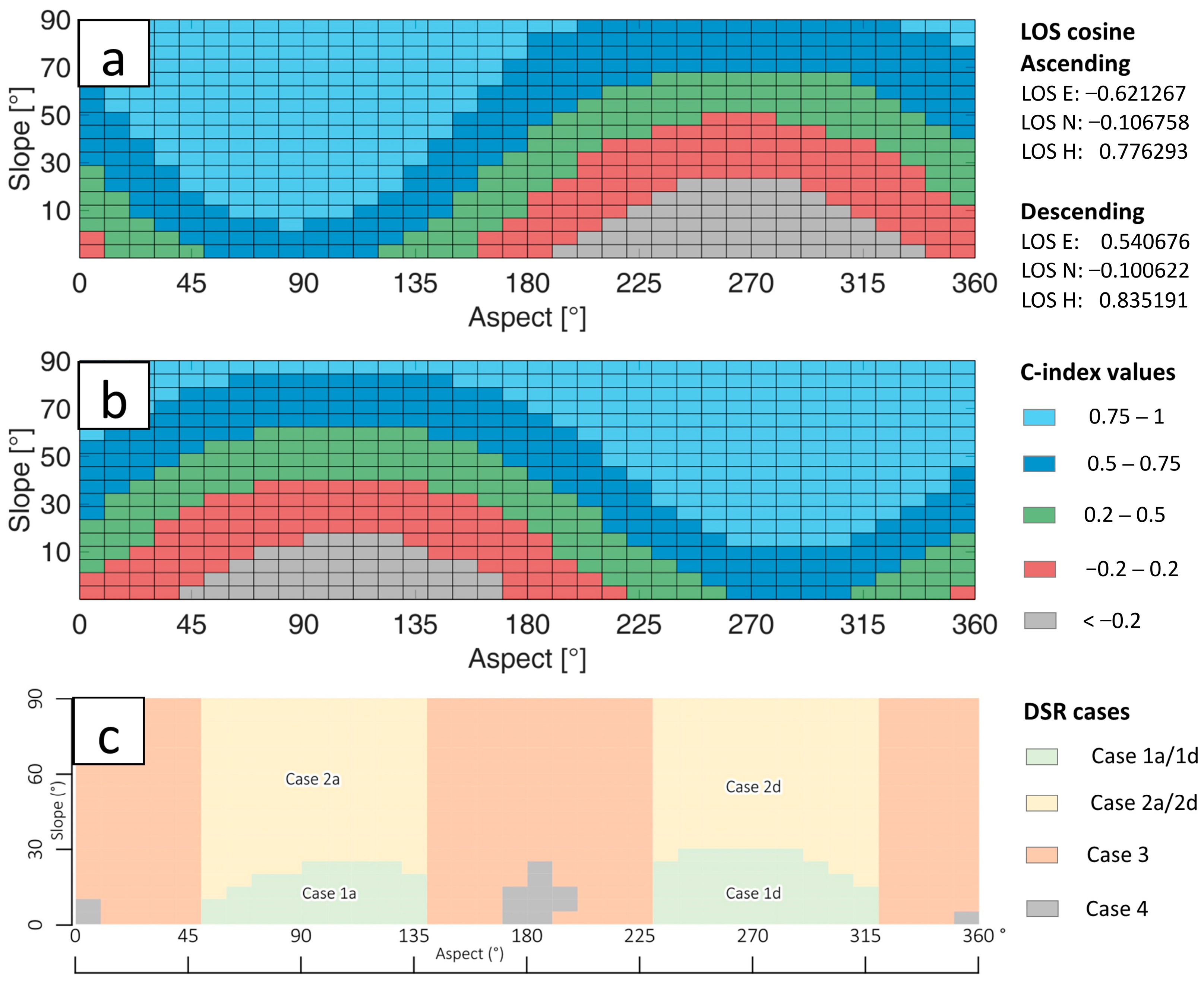
3.2. Data Suitability Ranking
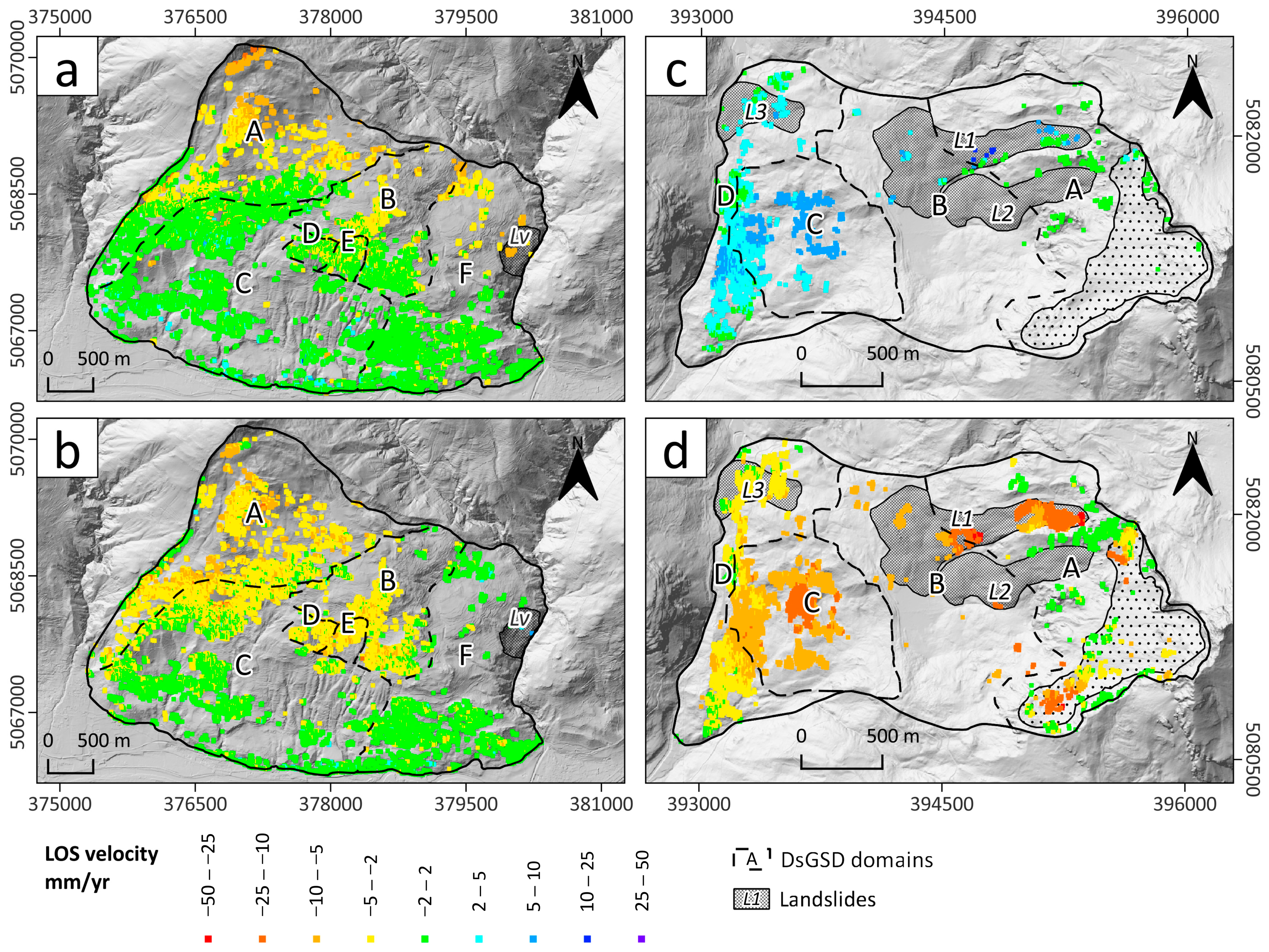
3.3. Ranked Ground Deformation Maps
4. Discussion
5. Conclusions
Supplementary Materials
Author Contributions
Funding
Data Availability Statement
Conflicts of Interest
References
- Mortara, G.; Sorzana, P.F. Fenomeni di deformazione graviativa profonda nell’arco alpino occidentale italiano; consideracioni lito-strutturali e morfologiche. Ital. J. Geosci. 1987, 106, 303–314. [Google Scholar]
- Ambrosi, C.; Crosta, G.B. Large sackung along major tectonic features in the Central Italian Alps. Eng. Geol. 2006, 83, 183–200. [Google Scholar] [CrossRef]
- Crosta, G.B.; Frattini, P.; Agliardi, F. Deep seated gravitational slope deformations in the European Alps. Tectonophysics 2013, 605, 13–33. [Google Scholar] [CrossRef]
- Frattini, P.; Crosta, G.B.; Allievi, J. Damage to Buildings in Large Slope Rock Instabilities Monitored with the PSInSARTM Technique. Remote Sens. 2013, 5, 4753–4773. [Google Scholar] [CrossRef]
- Béjar-Pizarro, M.; Notti, D.; Mateos, R.M.; Ezquerro, P.; Centolanza, G.; Herrera, G.; Bru, G.; Sanabria, M.; Solari, L.; Duro, J.; et al. Mapping Vulnerable Urban Areas Affected by Slow-Moving Landslides Using Sentinel-1 InSAR Data. Remote Sens. 2017, 9, 876. [Google Scholar] [CrossRef]
- Cignetti, M.; Godone, D.; Zucca, F.; Bertolo, D.; Giordan, D. Impact of Deep-seated Gravitational Slope Deformation on urban areas and large infrastructures in the Italian Western Alps. Sci. Total Environ. 2020, 740, 140360. [Google Scholar] [CrossRef]
- Pánek, T.; Klimeš, J. Temporal behavior of deep-seated gravitational slope deformations: A review. Earth-Sci. Rev. 2016, 156, 14–38. [Google Scholar] [CrossRef]
- Agliardi, F.; Crosta, G.B.; Frattini, P. Slow rock-slope deformation. In Landslides: Types, Mechanisms and Modeling; Clauge, J.J., Stead, D., Eds.; Cambridge University Press: Cambridge, UK, 2012; pp. 207–221. ISBN 978-1-107-00206-7. [Google Scholar]
- Giordan, D.; Cignetti, M.; Bertolo, D. The Use of Morpho-Structural Domains for the Characterization of Deep-Seated Gravitational Slope Deformations in Valle d’Aosta. In Advancing Culture of Living with Landslides; Springer International Publishing: Cham, Switzerland, 2017; pp. 59–68. [Google Scholar]
- Crippa, C.; Franzosi, F.; Zonca, M.; Manconi, A.; Crosta, G.B.; Dei Cas, L.; Agliardi, F. Unraveling Spatial and Temporal Heterogeneities of Very Slow Rock-Slope Deformations with Targeted DInSAR Analyses. Remote Sens. 2020, 12, 1329. [Google Scholar] [CrossRef]
- Morelli, S.; Pazzi, V.; Frodella, W.; Fanti, R. Kinematic reconstruction of a deep-seated gravitational slope deformation by geomorphic analyses. Geosciences 2018, 8, 26. [Google Scholar] [CrossRef]
- Demurtas, V.; Emanuele Orru, P.; Deiana, G. Active lateral spreads monitoring system in East-Central Sardinia. Eur. J. Remote Sens. 2022, 1–21. [Google Scholar] [CrossRef]
- Frattini, P.; Crosta, G.B.; Rossini, M.; Allievi, J. Activity and kinematic behaviour of deep-seated landslides from PS-InSAR displacement rate measurements. Landslides 2018, 15, 1053–1070. [Google Scholar] [CrossRef]
- Cignetti, M.; Godone, D.; Notti, D.; Zucca, F.; Meisina, C.; Bordoni, M.; Pedretti, L.; Lanteri, L.; Bertolo, D.; Giordan, D. Damage to anthropic elements estimation due to large slope instabilities through multi-temporal A-DInSAR analysis. Nat. Hazards 2023, 115, 2603–2632. [Google Scholar] [CrossRef]
- Crippa, C.; Valbuzzi, E.; Frattini, P.; Crosta, G.B.; Spreafico, M.C.; Agliardi, F. Semi-automated regional classification of the style of activity of slow rock-slope deformations using PS InSAR and SqueeSAR velocity data. Landslides 2021, 18, 2445–2463. [Google Scholar] [CrossRef]
- Cignetti, M.; Godone, D.; Notti, D.; Giordan, D.; Bertolo, D.; Calò, F.; Reale, D.; Verde, S.; Fornaro, G. State of activity classification of deep-seated gravitational slope deformation at regional scale based on Sentinel-1 data. Landslides 2023, 20, 2529–2544. [Google Scholar] [CrossRef]
- Wasowski, J.; Bovenga, F. Investigating landslides and unstable slopes with satellite Multi Temporal Interferometry: Current issues and future perspectives. Eng. Geol. 2014, 174, 103–138. [Google Scholar] [CrossRef]
- Herrera, G.; Gutiérrez, F.; García-Davalillo, J.C.; Guerrero, J.; Notti, D.; Galve, J.P.; Fernández-Merodo, J.A.; Cooksley, G. Multi-sensor advanced DInSAR monitoring of very slow landslides: The Tena Valley case study (Central Spanish Pyrenees). Remote Sens. Environ. 2013, 128, 31–43. [Google Scholar] [CrossRef]
- Casu, F.; Manzo, M.; Lanari, R. A quantitative assessment of the SBAS algorithm performance for surface deformation retrieval from DInSAR data. Remote Sens. Environ. 2006, 102, 195–210. [Google Scholar] [CrossRef]
- Cignetti, M.; Manconi, A.; Manunta, M.; Giordan, D.; De Luca, C.; Allasia, P.; Ardizzone, F. Taking Advantage of the ESA G-POD Service to Study Ground Deformation Processes in High Mountain Areas: A Valle d’Aosta Case Study, Northern Italy. Remote Sens. 2016, 8, 852. [Google Scholar] [CrossRef]
- Colesanti, C.; Wasowski, J. Investigating landslides with space-borne Synthetic Aperture Radar (SAR) interferometry. Eng. Geol. 2006, 88, 173–199. [Google Scholar] [CrossRef]
- Mondini, A.C.; Guzzetti, F.; Chang, K.T.; Monserrat, O.; Martha, T.R.; Manconi, A. Landslide failures detection and mapping using Synthetic Aperture Radar: Past, present and future. Earth-Sci. Rev. 2021, 216, 103574. [Google Scholar] [CrossRef]
- Noviello, C.; Verde, S.; Zamparelli, V.; Fornaro, G.; Pauciullo, A.; Reale, D.; Nicodemo, G.; Ferlisi, S.; Gulla, G.; Peduto, D. Monitoring Buildings at Landslide Risk With SAR: A Methodology Based on the Use of Multipass Interferometric Data. IEEE Geosci. Remote Sens. Mag. 2020, 8, 91–119. [Google Scholar] [CrossRef]
- Fornaro, G.; Lombardini, F.; Pauciullo, A.; Reale, D.; Viviani, F. Tomographic processing of interferometric SAR data: Developments, applications, and future research perspectives. IEEE Signal Process. Mag. 2014, 31, 41–50. [Google Scholar] [CrossRef]
- Ferretti, A.; Fumagalli, A.; Novali, F.; Prati, C.; Rocca, F.; Rucci, A. A new algorithm for processing interferometric data-stacks: SqueeSAR. IEEE Trans. Geosci. Remote Sens. 2011, 49, 3460–3470. [Google Scholar] [CrossRef]
- Fornaro, G.; Verde, S.; Reale, D.; Pauciullo, A. CAESAR: An approach based on covariance matrix decomposition to improve multibaseline--multitemporal interferometric SAR processing. IEEE Trans. Geosci. Remote Sens. 2014, 53, 2050–2065. [Google Scholar] [CrossRef]
- Fornaro, G.; Pauciullo, A.; Reale, D.; Verde, S. Multilook SAR tomography for 3-D reconstruction and monitoring of single structures applied to COSMO-SKYMED data. IEEE J. Sel. Top. Appl. Earth Obs. Remote Sens. 2014, 7, 2776–2785. [Google Scholar] [CrossRef]
- Fornaro, G.; Pauciullo, A.; Reale, D.; Verde, S. SAR coherence tomography: A new approach for coherent analysis of urban areas. In Proceedings of the 2013 IEEE International Geoscience and Remote Sensing Symposium-IGARSS, Melbourne, Australia, 21–26 July 2013; pp. 73–76. [Google Scholar]
- Cascini, L.; Fornaro, G.; Peduto, D. Advanced low- and full-resolution DInSAR map generation for slow-moving landslide analysis at different scales. Eng. Geol. 2010, 112, 29–42. [Google Scholar] [CrossRef]
- Plank, S.; Singer, J.; Minet, C.; Thuro, K. Pre-survey suitability evaluation of the differential synthetic aperture radar interferometry method for landslide monitoring. Int. J. Remote Sens. 2012, 33, 6623–6637. [Google Scholar] [CrossRef]
- Notti, D.; Herrera, G.; Bianchini, S.; Meisina, C.; García-Davalillo, J.C.; Zucca, F. A methodology for improving landslide PSI data analysis. Int. J. Remote Sens. 2014, 35, 2186–2214. [Google Scholar] [CrossRef]
- Verde, S.; Pauciullo, A.; Reale, D.; Fornaro, G. Multiresolution detection of persistent scatterers: A performance comparison between multilook GLRT and CAESAR. IEEE Trans. Geosci. Remote Sens. 2020, 59, 3088–3103. [Google Scholar] [CrossRef]
- Broccolato, M.; Paganone, M. Grandi Frane Permanenti Complesse—Schede Monografiche di Frane in Valle d’Aosta Analizzate con Tecnica PS—Attività B2C2 Rischi Idrogeologici e da Fenomeni Gravitativi—Progetto RiskNat; 2012. Available online: https://www.yumpu.com/it/document/view/30851951/schede-monografiche-di-frane-in-valle-daosta-analizzate-risknat (accessed on 10 October 2023).
- Trigila, A.; Iadanza, C.; Spizzichino, D. IFFI Project (Italian landslide inventory) and risk assessment. In Proceedings of the First World Landslide Forum; Springer: Berlin/Heidelberg, Germany, 2008; pp. 18–21. [Google Scholar]
- Martinotti, G.; Giordan, D.; Giardino, M.; Ratto, S. Controlling factors for deep-seated gravitational slope deformation (DSGSD) in the Aosta Valley (NW Alps, Italy). Geol. Soc. Lond. Spec. Publ. 2011, 351, 113–131. [Google Scholar] [CrossRef]
- Centro Funzionale Regione Autonoma Valle d’Aosta Catasto Dissesti. Available online: http://catastodissesti.partout.it/informazioni (accessed on 16 March 2020).
- Giardino, M. Analisi di Deformazioni Superficiali: Metodologie di Ricerca ed Esempi di Studio Nella Media Valle d’Aosta; University of Turin: Turin, Italy, 1995. [Google Scholar]
- Alberto, W.; Giardino, M.; Martinotti, G.; Tiranti, D. Geomorphological hazards related to deep dissolution phenomena in the Western Italian Alps: Distribution, assessment and interaction with human activities. Eng. Geol. 2008, 99, 147–159. [Google Scholar] [CrossRef]
- Giordan, D.; Cignetti, M.; Wrzesniak, A.; Allasia, P.; Bertolo, D. Operative Monographies: Development of a new tool for the effective management of landslide risks. Geosciences 2018, 8, 485. [Google Scholar] [CrossRef]
- Fornaro, G.; Pauciullo, A.; Serafino, F. Deformation monitoring over large areas with multipass differential SAR interferometry: A new approach based on the use of spatial differences. Int. J. Remote Sens. 2009, 30, 1455–1478. [Google Scholar] [CrossRef]
- Berardino, P.; Fornaro, G.; Lanari, R.; Sansosti, E. A new algorithm for surface deformation monitoring based on small baseline differential SAR interferograms. IEEE Trans. Geosci. Remote Sens. 2002, 40, 2375–2383. [Google Scholar] [CrossRef]
- Cigna, F.; Bianchini, S.; Casagli, N. How to assess landslide activity and intensity with Persistent Scatterer Interferometry (PSI): The PSI-based matrix approach. Landslides 2013, 10, 267–283. [Google Scholar] [CrossRef]
- Bonì, R.; Bordoni, M.; Colombo, A.; Lanteri, L.; Meisina, C. Landslide state of activity maps by combining multi-temporal A-DInSAR (LAMBDA). Remote Sens. Environ. 2018, 217, 172–190. [Google Scholar] [CrossRef]
- García-Davalillo, J.C.; Herrera, G.; Notti, D.; Strozzi, T.; Álvarez-Fernández, I. DInSAR analysis of ALOS PALSAR images for the assessment of very slow landslides: The Tena Valley case study. Landslides 2014, 11, 225–246. [Google Scholar] [CrossRef]
- Godone, D.; Garnero, G. The role of morphometric parameters in Digital Terrain Models interpolation accuracy: A case study. Eur. J. Remote Sens. 2017, 46, 198–214. [Google Scholar] [CrossRef]
- Fiorentini, N.; Maboudi, M.; Losa, M.; Gerke, M. Assessing resilience of infrastructures towards exogenous events by using ps-insar-based surface motion estimates and machine learning regression techniques. ISPRS Ann. Photogramm. Remote Sens. Spat. Inf. Sci. 2020, 4, 19–26. [Google Scholar] [CrossRef]
- Barla, G.; Antolini, F.; Barla, M.; Mensi, E.; Piovano, G. Monitoring of the Beauregard landslide (Aosta Valley, Italy) using advanced and conventional techniques. Eng. Geol. 2010, 116, 218–235. [Google Scholar] [CrossRef]
- Spreafico, M.C.; Agliardi, F.; Andreozzi, M.; Cossa, A.; Crosta, G.B. Large slow rock-slope deformations affecting hydropower facilities. In Proceedings of the EGU General Assembly Conference Abstracts, EGU2020-8288, Online, 4–8 May 2020; p. 8288. [Google Scholar]
- Bonì, R.; Bordoni, M.; Vivaldi, V.; Troisi, C.; Tararbra, M.; Lanteri, L.; Zucca, F.; Meisina, C. Assessment of the Sentinel-1 based ground motion data feasibility for large scale landslide monitoring. Landslides 2020, 17, 2287–2299. [Google Scholar] [CrossRef]
- Notti, D.; Meisina, C.; Zucca, F.; Colombo, A. Models to predict Persistent Scatterers data distribution and their capacity to register movement along the slope. In Proceedings of the Fringe Workshop, Frascati, Italy, 19–23 September 2011; pp. 19–23. [Google Scholar]
- Barra, A.; Reyes-Carmona, C.; Herrera, G.; Galve, J.P.; Solari, L.; Mateos, R.M.; Azañón, J.M.; Béjar-Pizarro, M.; López-Vinielles, J.; Palamà, R.; et al. From satellite interferometry displacements to potential damage maps: A tool for risk reduction and urban planning. Remote Sens. Environ. 2022, 282, 113294. [Google Scholar] [CrossRef]
- Dai, K.; Deng, J.; Xu, Q.; Li, Z.; Shi, X.; Hancock, C.; Wen, N.; Zhang, L.; Zhuo, G. Interpretation and sensitivity analysis of the InSAR line of sight displacements in landslide measurements. GIScience Remote Sens. 2022, 59, 1226–1242. [Google Scholar] [CrossRef]
- Ren, T.; Gong, W.; Gao, L.; Zhao, F.; Cheng, Z. An Interpretation Approach of Ascending—Descending SAR Data for Landslide Identification. Remote Sens. 2022, 14, 1299. [Google Scholar] [CrossRef]
- Chiesa, S.; Fornero, I.; Frassoni, A.; Zanchi, A.; Mazza, G.; Zaninetti, A. Gravitational instability phenomena concerning a hydroelectric plant in Italy. In Proceedings of the 7th ISRM Congress, Aachen, Germany, 16–20 September 1991. [Google Scholar]


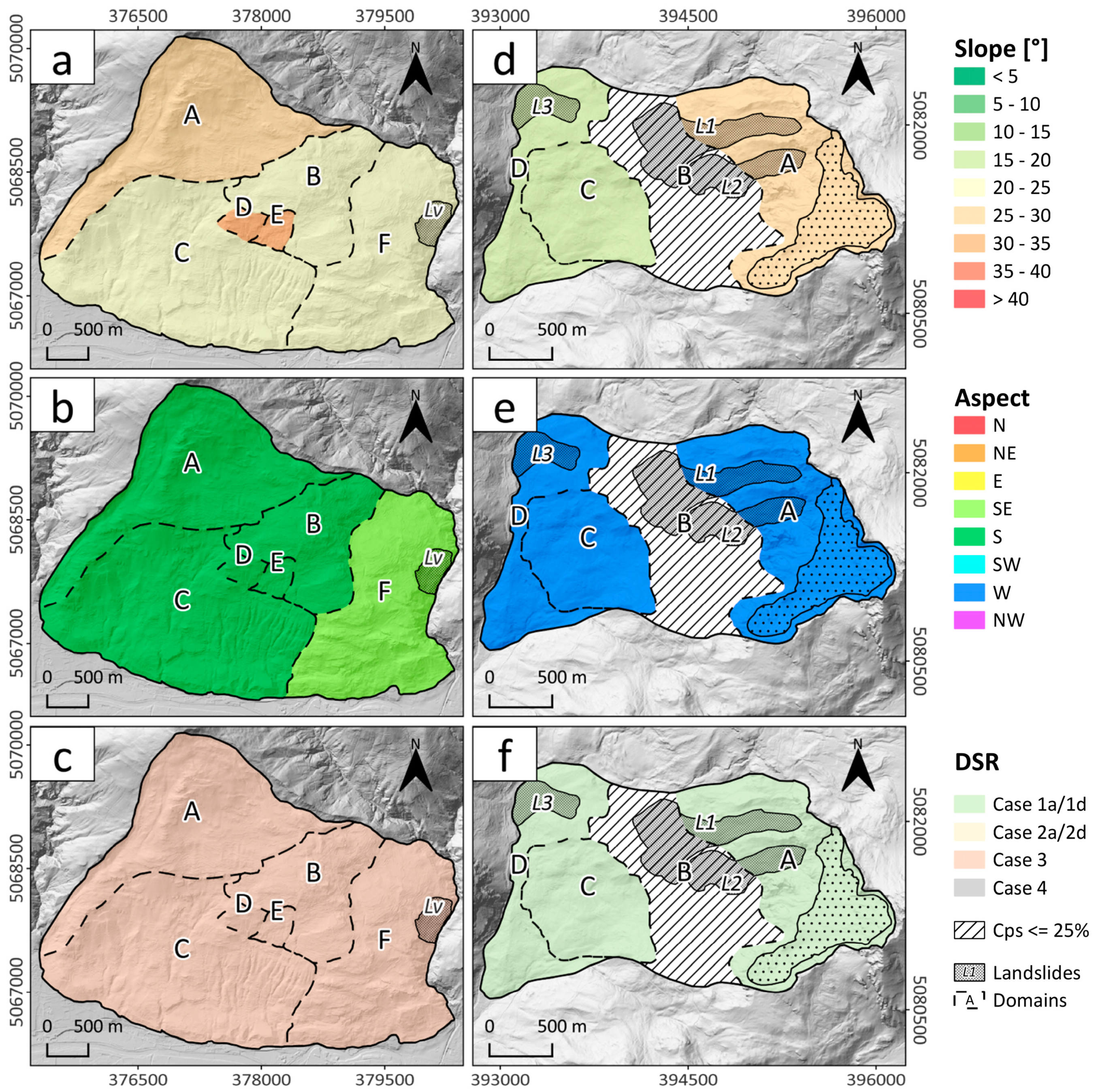
| Aspect Class | Slope Threshold | C-Index Combination | Case | Qualitative Ranking | Velocity Type Priority |
|---|---|---|---|---|---|
| 45–135° | <30° | Ca > 0.2 and Cd < −0.2 | Case 1a | High | Vew–Vv; VLOSa; VSLOPE, VLOSd |
| 225–315° | <30° | Ca < −0.2 and Cd > 0.2 | Case 1d | High | Vew–Vv; VLOSd; VSLOPE, VLOSa |
| 45–135° | >30° | Ca > 0.2 | Case 2a | Medium–High | VLOSa; VSLOPE |
| 225–315° | >30° | Cd > 0.2 | Case 2d | Medium–High | VLOSd; VSLOPE |
| (135–225°) or (0–45°) or (315–360°) | - | Ca > 0.2 or Cd > 0.2 | Case 3 | Low | VSLOPE; Vv; Vew |
| - | - | −0.2 ≤ Ca ≥ 0.2 and −0.2 ≤ Cd ≥ 0.2 | Case 4 | Worst case | None |
Disclaimer/Publisher’s Note: The statements, opinions and data contained in all publications are solely those of the individual author(s) and contributor(s) and not of MDPI and/or the editor(s). MDPI and/or the editor(s) disclaim responsibility for any injury to people or property resulting from any ideas, methods, instructions or products referred to in the content. |
© 2023 by the authors. Licensee MDPI, Basel, Switzerland. This article is an open access article distributed under the terms and conditions of the Creative Commons Attribution (CC BY) license (https://creativecommons.org/licenses/by/4.0/).
Share and Cite
Cardone, D.; Cignetti, M.; Notti, D.; Godone, D.; Giordan, D.; Calò, F.; Verde, S.; Reale, D.; Sansosti, E.; Fornaro, G. Slope-Scale Evolution Categorization of Deep-Seated Slope Deformation Phenomena with Sentinel-1 Data. Remote Sens. 2023, 15, 5440. https://doi.org/10.3390/rs15235440
Cardone D, Cignetti M, Notti D, Godone D, Giordan D, Calò F, Verde S, Reale D, Sansosti E, Fornaro G. Slope-Scale Evolution Categorization of Deep-Seated Slope Deformation Phenomena with Sentinel-1 Data. Remote Sensing. 2023; 15(23):5440. https://doi.org/10.3390/rs15235440
Chicago/Turabian StyleCardone, Davide, Martina Cignetti, Davide Notti, Danilo Godone, Daniele Giordan, Fabiana Calò, Simona Verde, Diego Reale, Eugenio Sansosti, and Gianfranco Fornaro. 2023. "Slope-Scale Evolution Categorization of Deep-Seated Slope Deformation Phenomena with Sentinel-1 Data" Remote Sensing 15, no. 23: 5440. https://doi.org/10.3390/rs15235440
APA StyleCardone, D., Cignetti, M., Notti, D., Godone, D., Giordan, D., Calò, F., Verde, S., Reale, D., Sansosti, E., & Fornaro, G. (2023). Slope-Scale Evolution Categorization of Deep-Seated Slope Deformation Phenomena with Sentinel-1 Data. Remote Sensing, 15(23), 5440. https://doi.org/10.3390/rs15235440