Concept of a Satellite Cross-Calibration Radiometer for In-Orbit Calibration of Commercial Optical Satellites

Abstract

The satellite Earth observation (EO) sector is burgeoning with hundreds of commercial satellites being launched each year, delivering a rich source of data that could be exploited for societal benefit. Data streams from the growing number of commercial satellites are of variable quality, limiting the potential for their combined use in science applications that need long time-series data from multiple sources. The quality of calibration performed on optical sensors onboard many satellite systems is highly variable due to calibration methods, sensor design, mission objective, budget, or other operational constraints. A small number of currently operating well-characterised satellite systems with onboard calibration, such as Landsat-8/9 and Sentinel-2, and planned future missions, like the NASA Climate Absolute Radiance and Refractivity Observatory (CLARREO) Pathfinder, the European Space Agency (ESA)’s Traceable Radiometry Underpinning Terrestrial and Helio Studies (TRUTHS), and LIBRA from China, are considered benchmarks for optical data quality due to their traceability to international measurement standards. This paper describes the concept of a space-based transfer calibration radiometer called the Satellite Cross-Calibration Radiometer (SCR) that would enable the calibration parameters from satellites such as Landsat-8/9, Sentinel-2, or other benchmark systems to be transferred to a range of commercial optical EO satellite systems while in orbit. A description of the key characteristics of the SCR to successfully operate in orbit and transfer calibration from reference systems to client systems is presented. A system like the SCR in orbit could complement SI-Traceable satellites (SITSats) to improve data quality and consistency and facilitate the interoperable use of data from multiple optical sensor systems for delivering higher returns on the global investment in EO.

1. Introduction

The number of Earth observation (EO) missions is growing rapidly, generating ever-increasing volumes of satellite data with immense potential for global applications across multiple science domains. Sustainable access to quality EO data from multiple satellite systems is fundamental for many environmental monitoring programs ranging in scale from regional to global. The ability to use data interoperably from multiple satellite systems from both the civil and commercial sectors enhances the frequency of observations for time-series applications where transient events could be missed due to fewer opportunities for observation by a single system. Scientists often use multiple optical remote sensing sensor systems to obtain datasets for their research, which makes it necessary to comprehend how differences between the datasets can affect the results for various scientific purposes. In this context, the term “optical” refers to sensor systems that function in the solar reflective domain, covering the wavelength range from 400 nm to 2500 nm. Variation between sensors due to spectral differences or radiometric uncertainty can be addressed by cross-calibration. Through cross-calibration, scientists can better understand the uncertainties associated with data products from any particular sensor. Consequently, they can use these different datasets alongside one another for their research applications. Interoperable multi-sensor data from civil and commercial satellites also provide redundancy in the event that data are affected by environmental factors such as cloud cover. However, the potential for combined use of multi-sensor EO data from a range of commercial optical systems remains largely underutilised due to their unknown quality. Space-based cross-calibration using the concept of a Satellite Cross-calibration Radiometer, hereafter referred to as SCR, could help address this issue.

Consistent data quality is the key to interoperability; it would be challenging to bring data from different sources together for synergistic use unless their quality is comparable. Australia’s Earth Observation from Space Roadmap [1] identified data quality assurance as one of five focus areas for the Australian EO sector. A recent Australian report on the calibration of EO data noted that trust and quality assurance of data are fundamental for the Australian EO sector to thrive and are critical to industry, government, and national security programs [2]. Several international studies have also expressed the need to improve satellite data quality and accuracy [3,4,5,6]. The Quality Assurance Framework for Earth Observation (QA4EO) was established and endorsed by the Committee on Earth Observation Satellites (CEOS) to meet a requirement identified by the Group on Earth Observations (GEO) to enable interoperability and quality assessment of EO data [7]. The guiding principle for data quality within the QA4EO framework is that all data and derived products must have an associated quality indicator based on a quantitative assessment of their traceability to reference standards, ideally the International System of Units (SI). The Global Space-based Inter-Calibration System (GSICS) is an international collaborative effort aimed at ensuring consistent accuracy among space-based observations worldwide for climate monitoring, weather forecasting, and environmental applications. The GSICS was initiated in 2005 by the World Meteorological Organization (WMO) and the Coordination Group for Meteorological Satellites (CGMS) to monitor, improve, and harmonise the quality of observations from operational weather and environmental satellites [8,9]. The work of the GSICS has helped many operational satellite systems, but similar benefits are yet to be fully realised for a range of commercial ‘New Space’ systems.

Civil and commercial EO satellite systems operate optical sensors that are calibrated using a combination of approaches, usually including pre-launch characterisation in a laboratory, on-board calibration equipment, and vicarious calibration using well-instrumented or well-characterised ground-based sites or the moon. The extent, rigour, and nature of calibration performed on sensor systems can be highly variable. This leads to the quality of data generated by the sensors being highly variable, constraining or limiting the combination of multi-sensor data for use in high-end applications involving quantitative analysis. Well-calibrated data, on the other hand, can provide better information and insights, as illustrated by the application examples in Figure 1 and Figure 2.

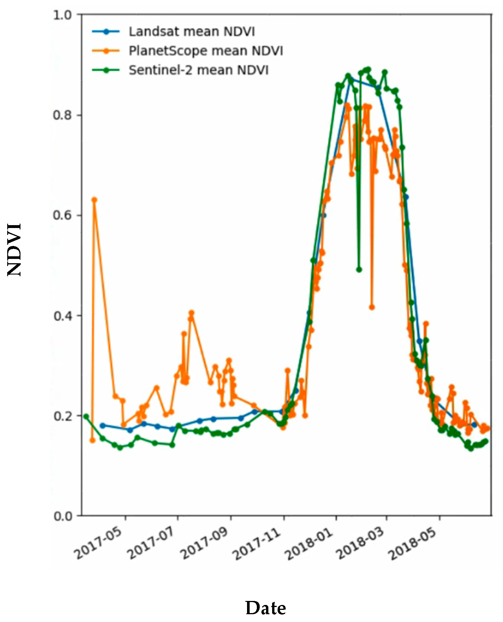
Figure 1 shows a time series of Normalised Difference Vegetation Index (NDVI) derived separately from Landsat-8, Sentinel-2, and PlanetScope data over an agricultural site in New South Wales, Australia (Bishop-Taylor, R., Geoscience Australia, Personal Communication, 2022). The plot highlights differences in the individual NDVI profiles generated from data acquired by the three satellite systems. The combined use of NDVI from the three sensor systems is limited due to inherent differences in the source data. Effective cross-calibration of data from these sensors could minimise such differences and render them comparable to each other.

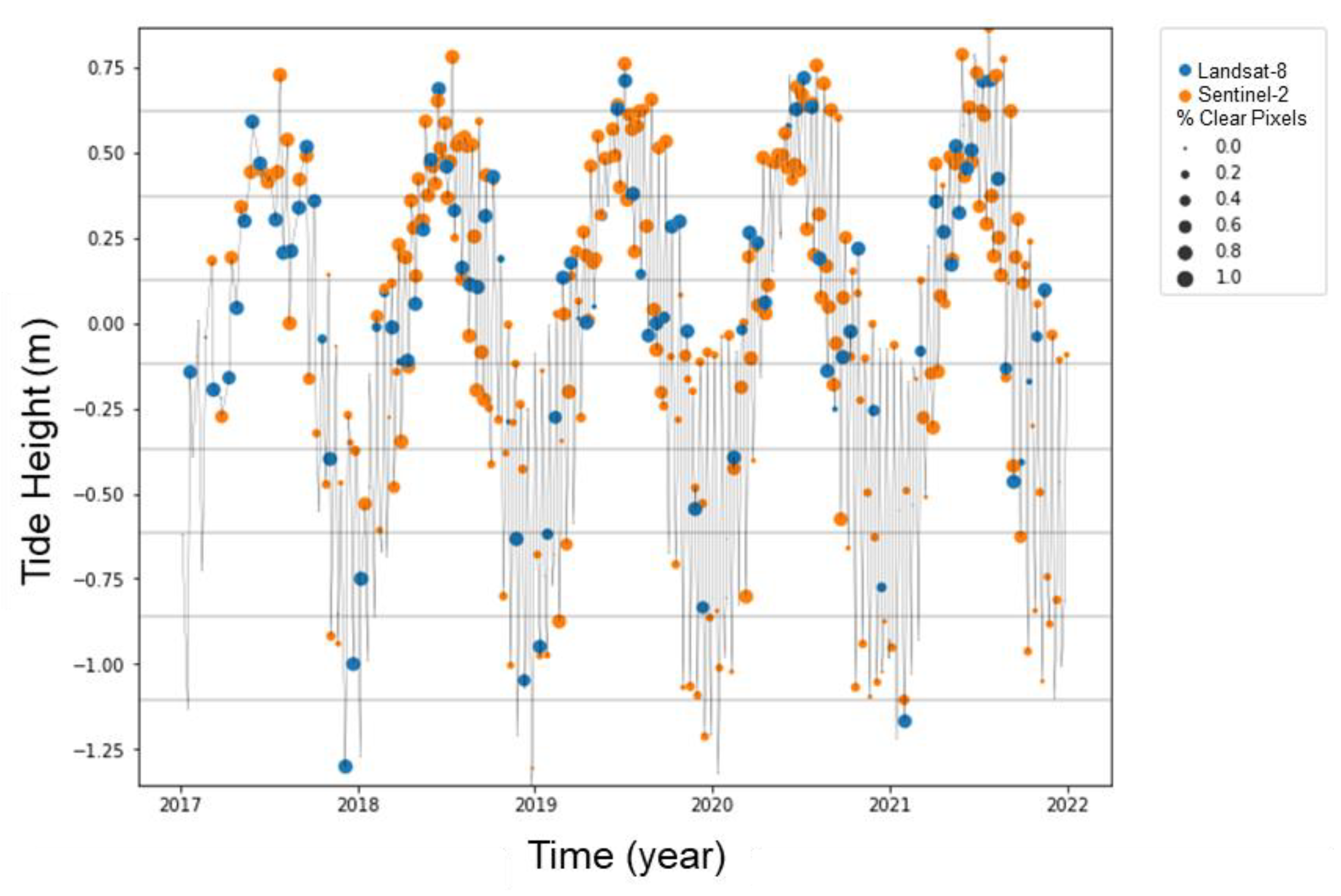
Figure 2 below highlights a case study from Australia demonstrating the benefits of synergistic applications of well-calibrated multi-sensor data. A study by Bishop-Taylor et al. [10] combined global tidal modelling with a 30-year archive of calibrated Landsat data to generate a National Intertidal Digital Elevation Model (NIDEM). Preliminary work on extending the NIDEM has shown that by combining calibrated Sentinel-2 and Landsat data, observations that best represent the full tidal range in coastal northern Australia can be achieved. It can be seen from Figure 2 that most of the Sentinel-2 observations at low tide represent a low percentage of clear pixels due to the effect of cloud or glint (smaller dots), but the Landsat-8 data with clearer observations at low tide make up for the shortfall in higher resolution Sentinel-2 observations. Similarly, at high tide, Landsat observations are sparse, but there is a higher density of Sentinel-2 observations. The combined use of these two datasets enables the capture of the intertidal zone extent and provides a more complete picture of the tidal dynamics in a shorter time period.

Comparing or combining data from the same satellite acquired at different times is also challenging when basic mechanisms for calibrating measurements that generate the data are lacking. This inconsistency substantially diminishes the scientific value of data from these systems for various applications, including climate change, agriculture, geology, hydrology, and natural disaster support. A few satellite systems such as the Climate Absolute Radiance and Refractivity Observatory (CLARREO) Pathfinder from the National Aeronautics and Space Administration (NASA), the European Space Agency (ESA) Traceable Radiometry Underpinning Terrestrials and Helio Studies (TRUTHS), and LIBRA from China—often referred to as ‘SI-Traceable Satellites (SITSats)’ due to their capability to provide uncertainties traceable to the international SI standard—are planned for launch [11,12,13]. The SITSat missions are designed to deliver highly accurate climate monitoring data, including Essential Climate Variables (ECVs), with SI-traceable radiometric uncertainties well below 1%, to qualify them as ‘metrology laboratories in space.’ As the design objective of SITSats is to achieve high-accuracy climate monitoring data, their orbits are not necessarily chosen for simultaneous or near-simultaneous observations that coincide with many ‘New Space’ or commercial systems. For example, the CLARREO Pathfinder mission would be deployed on the International Space Station (ISS), which might constrain its ability to perform coincident observations with a large number of EO satellites. Also, TRUTHS is planned for a true-polar orbit; however, it will have fewer simultaneous nadir overpasses (SNOs) through much of the year due to that.

The concept for the SCR can be traced back to a United States Geological Survey (USGS) National Land Imaging (NLI) program architecture study, which identified the need for a new generation of land remote sensing instruments with improved temporal, spectral, and spatial performance, supported by a cross-calibration radiometer [14]. The concept was further evolved in a technical feasibility study conducted in Australia [15]. The SCR would be an in-orbit transfer radiometer focused on transferring top-of-atmosphere (TOA) radiance from a reference or benchmark instrument to one or more client instruments in orbit. To achieve this, the SCR hyperspectral instrument must have the spectral and spatial capability to optimally match both the reference and client instruments and be placed in an orbit that maximises opportunities for cross-calibration with several reference and client satellite systems. In simulation studies using hyperspectral data from a Deutsches Zentrum für Luft- und Raumfahrt (DLR) Earth Sensing Imaging Spectrometer (DESIS) instrument as a surrogate for the SCR, it was shown that effective calibration transfer from a reference system such as Landsat 8 could be achieved [16]. A study by Roithmayr et al. [17] analysed opportunities for the CLARREO Pathfinder to be deployed on the ISS to intercalibrate instruments onboard the spacecraft in low Earth orbit and geosynchronous Earth orbit. 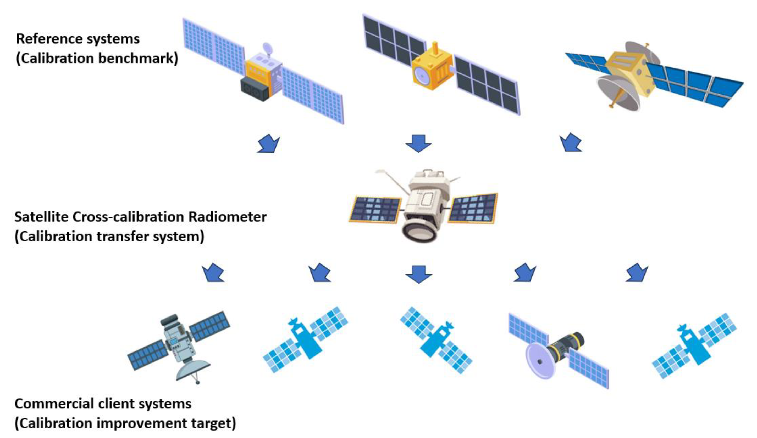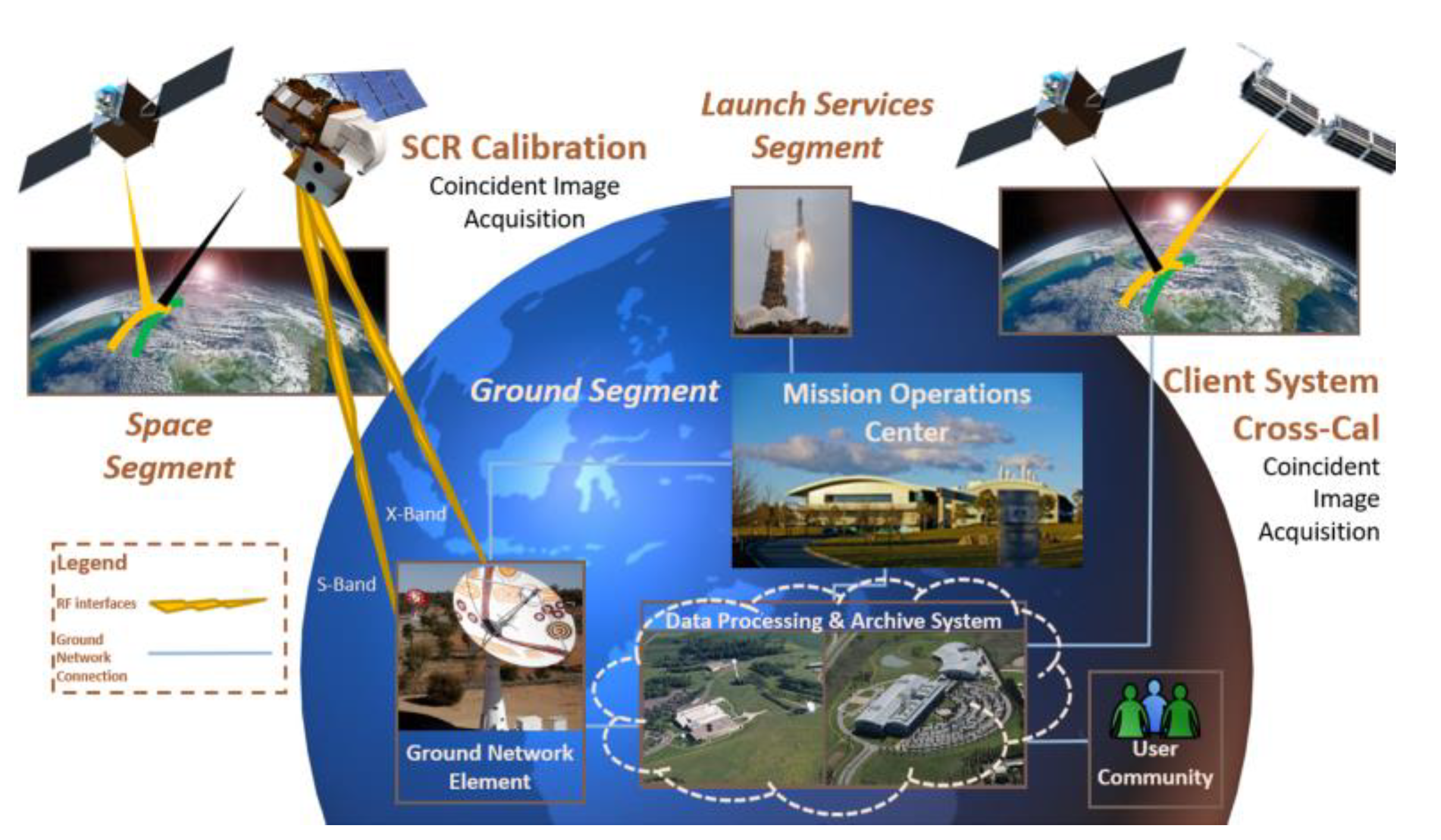Figure 3 is a schematic representing the process of the calibration transfer between reference and client systems that would be enabled by the SCR. Reference systems currently in orbit include satellites such as Landsat 8/9 or Sentinel-2 that are well characterised pre-launch, with their calibration performance monitored in-orbit.

The SCR concept presented here describes how space-based cross-calibration of multiple commercial optical sensors would enable better consistency and quality of data by minimising differences in calibration approaches. The SCR would enable the generation of high-quality data across numerous optical imaging satellite systems and maximise the data utilisation potential of these EO systems.

2. SCR Overview

Understanding and addressing differences and changes in radiometric accuracy regarding gains and biases is important for multi-sensor data to be used interoperably. Interoperability in this context is the combined use of complementary sensors to achieve a combined data stream to be used with a particular application, with known uncertainties. Many science applications also require data interoperability for long-term trending and information derived from opportunistic observations. Space agencies, including NASA and ESA, recognise the need for a space-based cross-calibration capability to unlock the potential of data from different instruments to be interoperable. SITSats are expected to make substantial contributions to address this need. Hyperspectral instruments, which typically cover the wavelength range for remote sensing systems in the visible/near infrared (VIS/NIR) regions, would be the main mechanism on SITSats and the SCR for transferring calibration from a reference source in orbit to other optical instruments in orbit that can benefit from the cross-calibration. The key SCR objectives would be to

• Effectively transfer TOA radiance measurements from a reference or benchmark satellite to one or more client satellites.
• Through effective cross-calibration, enable improved quality, consistency, and interoperability of data from multiple EO missions globally.
• Facilitate the generation of science-quality data streams from multiple satellites to support a broader range of EO applications.
• Consolidate procedures for routine space-based cross-calibration that can be applied to the development of future missions.

SCR Concept

Space-based calibration transfer to in-orbit satellites using the SCR is based on near-SNOs of a reference satellite and the SCR over a common area. An overview by Chander, G. et al. provides several approaches used for space-based satellite intercalibration, including SNOs [18,19,20]. SNOs are observations of the same areas of the Earth at nearly the same time, generally within ±20 min, to minimise measurement differences due to variations in sun angle and atmospheric conditions. A process of spectral synthesis is then used to simulate the multispectral bands from the reference satellite using the data from the SCR hyperspectral bands. This is a common technique that can be used to emulate multispectral bands [16]. The reference satellite’s calibration can then be transferred from the SCR to a client satellite using the same process. Knowledge of the reference and client satellite systems’ Relative Spectral Response (RSR) functions is critical for spectral synthesis. Additional processes that form part of the calibration transfer workflow, such as geometric co-registration, spatial harmonisation, cloud screening, and outlier removal, are also applied and described in [16]. The high-level SCR concept is illustrated in Figure 4 and described in detail later in this section. As this paper focuses on the concept of the SCR rather than its operational aspects, a detailed analysis of the SCR system architecture is beyond the scope of this paper; however, a notional system architecture for the SCR is provided in Section 5.

The cost and complexity of the hyperspectral SCR instrument depend on sensor parameters such as spectral resolution, spectral range, spatial resolution, and signal-to-noise ratio (SNR). The results of performance trade-offs between these sensor parameters were quantified in a study that showed minimal impact on cross-calibration quality, indicating the possibility of using a low-cost SCR hyperspectral instrument for cross-calibration [16]. A key aspect of the SCR concept would be the ability to integrate the reference and client RSR functions to generate the synthetic images for use in the process of cross-calibration. Interoperability between the two observing systems could thus be improved.

Table 1. Nominal SCR cross-calibration with a reference system.

Step	Description
1	Identify coincident imaging windows between SCR and the reference satellite system over land areas imaged by both satellites nominally within ±20 min of each other.
2	Select matching near-coincident imagery from both satellites to use for cross-calibration, avoiding data that are affected by clouds or other atmospheric phenomena.
3	Use SCR hyperspectral bands to synthesise reference satellite data based on reference satellite RSR functions.
4	Compare synthesised SCR data to reference satellite data on a per-band basis to determine differences in gain and bias, ensuring geodetic/spatial registration between the datasets.
5	Examine the resulting differences with reference satellites to re-calibrate SCR response for product generation, including modifications in ground algorithm parameters. This process continues regularly throughout the system’s lifetime.
6	Repeat as needed to ensure SCR generates well-calibrated TOA data during the entire mission life to account for sensor variation over time.

SCR, Satellite Cross-calibration Radiometer; RSR, relative spectral response; TOA, top of atmosphere.

and

Table 2. Nominal SCR client cross-calibration with a client system.

Step	Description
1	Retrieve synthesised multispectral data from the SCR spectral synthesis.
2	Develop gain and bias coefficients for each client band, using RSR function for client system.
3	Make new gain and bias parameters available for client data processing.
4	Generate client TOA radiance products with SCR bias parameters applied or appended.

SCR, Satellite Cross-calibration Radiometer; RSR, relative spectral response; TOA, top of atmosphere.

provide a step-by-step breakdown of the cross-calibration between the SCR and the reference and client systems, respectively.

3. SCR Instrument Requirements

This section covers the requirements for the instrument characteristics that would enable the SCR cross-calibration objectives to be effectively achieved. The driving calibration requirements consist of radiometric, geometric, and spatial requirements and are constrained by time intervals between calibration events. Typical hyperspectral instruments designed for specific imaging applications attempt to maximise the number of independent spectral classes that can be discerned in a dataset [16]; this requires effort to enhance the SNR and strive for high spatial resolution and fine spectral resolution. In contrast, the SCR hyperspectral imager must be able to effectively transfer TOA radiance from a reference or benchmark instrument to a client instrument; this requires a slightly different set of criteria to be applied. In

Table 3. SCR hyperspectral instrument parameters compared to typical hyperspectral imaging instruments.

Parameter	Typical Hyperspectral Instrument	SCR Hyperspectral Instrument
Spectral Range	Must cover atmospheric windows and spectral regions of interest relevant for the application.	Must cover spectral range of reference and client instruments.
Spectral Sampling Interval (SSI) and Resolution, full width at half maximum (FWHM)	Must be small enough to discern spectral features of interest.	Spectral sampling and resolution must be several times finer than RSR (FWHM and shape) being simulated. Must be tailored to achieve small TOA spectral radiance emulation errors (refer to [17]).
Spatial Sampling (Ground Sampling Distance) and Resolution	Spatial resolution sized for material classification and relatively high Modulation Transfer Function (MTF)@Nyquist is desired to decrease spectral mixing.	Less important than typical. Can be coarse. Spatial resolution tailored for area coverage and can be increased to improve SNR. May have limited use of RadCalNet sites if spatial resolution becomes too large.
Signal-to-Noise Ratio (SNR)	High SNR required to maintain high dimensionality for spectral classification.	Less important than typical systems because multiple samples can be averaged to increase the SNR and reduce the uncertainty in cross-calibration.
Swath/Revisit	Application dependent, but larger is preferred.	Decreased swath minimises the impact of the bidirectional reflectance distribution function (BRDF) and uses smaller Focal Plane Arrays (FPA). Larger swath increases cross-calibration opportunities.
Radiometry	Important for atmospheric correction.	Stability is critical.

SCR, Satellite Cross-calibration Radiometer; SSI: spectral sampling interval: FWHM, full width half maximum; RSR: relative spectral response, TOA, top of atmosphere, MTF: modulation transfer function, SNR: signal to noise ratio, BRDF: bidirectional reflectance distribution function, FPA: focal plane array.

, several SCR parameters, including spectral, spatial, and radiometric properties, are presented and compared to those of typical hyperspectral instruments designed for specific imaging applications, such as EO-1 Hyperion, Hyperspectral Imager for the Coastal Ocean (HICO), TianGong-1, PRISMA, DESIS, HISUI, Environmental Mapping and Analysis Program (EnMAP), Earth Surface Mineral Dust Source Investigation (EMIT), SHALOM, HypXIM, and also airborne hyperspectral instruments: Airborne Visible InfraRed Imaging Spectrometer—Next Generation (AVIRIS-NG), Portable Remote Imaging Spectrometer (PRISM), and Coral Reef Airborne Laboratory (CORAL). The SCR instrument parameters outlined below highlight the specific requirements to effectively perform the function of a calibration transfer radiometer in space.

A team from the Earth Resources Observation and Science (EROS) Center of the USGS developed a set of draft specifications for an affordable hyperspectral instrument that could be implemented on a small satellite as part of the SCR mission. The development of the draft specifications was also supported by simulation studies in order to understand the impact of these requirements on cross-calibration uncertainty [16]. Based on the work conducted at the USGS, a nominal set of threshold and goal specifications for various parameters associated with a hyperspectral instrument on the SCR are given in

Table 4. Nominal instrument specifications for SCR.

Category	Parameter	Specification T: Threshold G: Goal
Spatial	Swath at nadir	>64 km
	Spatial sampling (across and along track at nadir) GSD	100–120 m
	MTF@Nyquist	0.1–0.35
	Field of view (FOV)	>5.68 deg
	Geometric accuracy	<a few km
Spectral	Spectral range	T: 400–2400 nm G: 350–2400 nm
	Spectral sampling interval	T: <5 (400–900 nm) <10 (900–2500 nm) G: <3 (400–900 nm) <6 (900–2500 nm)
	Spectral resolution, full width at half maximum (FWHM)	1–2 × Sampling interval nm
	Spectral calibration accuracy	0.1 × FWHM nm
Radiometric	Radiometric accuracy (SI)
	Pre-flight	T: <2%
	On-orbit	G: <4%
	Transfer Calibration Uncertainty (TCU) Reference to SCR	<1% (after n collects)
	Radiometric stability	T: 0.2% over 7 days G: 0.2% over 30 days
	SNR	>~20–30 Sample number dependent, e.g., greater than 100 independent samples
	Polarisation sensitivity	T: 5% G: 3%
	Linearity (over 90% of dynamic range)	T: 0.5% G: 0.3%
	Lsat (saturation radiance)	Defined in Section 3.3 as 1.15 times the radiance of a 100% Lambertian target at a 10 km altitude and 0° solar zenith angle
Orbit	Altitude	645 km
	Inclination angle	97.75 deg
	Nadir equatorial repeat time	48 days
	Orbital equatorial crossing time	10:20 a.m.

km: kilometre; GSD: ground sample distance, m: metre, SSI: spectral sampling interval: MTF: modulation transfer function, FOV: field of view, deg: degree, nm: nanometre, FWHM, full width half maximum; SI: spectral interval, TCU: transfer calibration uncertainty, ms: milliseconds, Lsat: saturated radiances, AM: ante meridian.

. Threshold specifications are minimum required values, and goal specifications are preferred values. The nominal instrument specifications for the SCR were used in the analyses described in this paper. Justification for specifying these values is provided In later sections of the paper.

3.1. Spatial Requirements

The factors considered when selecting the swath and spatial resolution values for the SCR, listed in Table 4, are described here.

3.1.1. Ground Sampling and Swath

The availability of Commercial Off-The-Shelf (COTS) Focal Plane Arrays (FPAs), particularly for shortwave infrared (SWIR) sensors, is restricted to common formats (e.g., 640 × 480), which limits the ground sampling distance (GSD) range and swath for most instrument types. A larger GSD could be considered if the instrument size needs to be reduced because the foreoptic telescope focal length decreases. Nadir viewing is preferred as a very large swath increases off-angle viewing and bidirectional reflectance distribution function (BRDF) effects. For example, TRUTHS and CLARREO Pathfinder have swaths of less than 100 km.

Cross-calibrations are not very sensitive to GSD and point spread function (PSF); for example, TRUTHS and CLARREO Pathfinder are designed for up to 500 m GSD [12]. Calibration using ground-based vicarious calibration sites, including the RadCalNet network [21], benefit from a smaller GSD because non-uniformity errors increase with GSDs over 100 m, as shown in [22]. Vicarious calibration using RadCalNet sites could achieve an SI-traceable radiometric accuracy goal of <4% [23]. Considering the above factors, a swath of 64 km and a nominal GSD of 100 m were selected. The values are consistent with available COTS FPAs.

3.1.2. Modulation Transfer Function and Field of View

Modulation Transfer Function (MTF)@Nyquist was chosen as a measure of image sharpness independent of GSD and is more commonly used than PSF or edge slope as used for Landsat. The MTF@Nyquist value must balance the aliasing that occurs at higher values and the blurring that occurs at lower values. Blurring increases spectral and spatial mixing and affects hyperspectral applications. On the other hand, too much aliasing could result in artifacts for some scene types [22]. For the SCR, the impact of aliasing or blurring could be minimised by applying scene and pixel selection criteria. For the SCR, the risk of aliasing or blurring can be minimised by ensuring that MTF@Nyquist values lie between 0.1 and 0.35.

3.1.3. Geometric Accuracy

As outlined in Table 4, a GSD between 100 and 120 m and swath width of 64 km translates to a field of view (FOV) of ±2.84 degrees and instantaneous field of view (IFOV) of 155 microrads, assuming an orbit altitude of 645 km. As the geometric accuracy requirement is less than a few kilometres, co-registration to a reference imager such as the Landsat or Sentinel-2 is relatively straightforward, as long as there is overlap [16]. DESIS, for example, co-registers to a Landsat base image. The intention would be to use a Worldwide Reference System (WRS) similar to that used for Landsat. The WRS is a global system that catalogues remote sensing data by path and row numbers. The gridding scheme would follow the row–path scheme. This system has proven valuable for cataloguing, referencing, and daily use of imagery transmitted from reference sensors such as Landsat. The row refers to the latitudinal centre line of a frame of imagery, where the combination of a path and row number uniquely defines the nominal scene centre. Using the path and row system will allow for easier coincident scene selections and spatial matching to reference satellites.

3.2. Spectral Requirements

3.2.1. Spectral Range

The SCR’s threshold spectral range is 400–2400 nm, which covers the spectral range of most current and planned shortwave multispectral and hyperspectral satellite imaging systems. Note that we are not including thermal infrared (TIR) bands in the intended spectral range due to the additional complexity, size, mass, and volume requirements needed. The goal spectral ranges could be increased by lowering the short wavelength end to 350 nm to accommodate additional hyperspectral imagers [15].

3.2.2. Spectral Bandwidth

Fine hyperspectral resolution is critical to achieve accurate spectral synthesis of multispectral bands. The SCR’s spectral resolution must be small enough to achieve small TOA spectral radiance emulation errors, which is also dependent on the multispectral bandwidths to be synthesised. EO satellites such as Sentinel-2 also have instruments with narrow bands [17], which are not easily or accurately synthesised with a spectral resolution of 10 nm typical for many hyperspectral imagers. 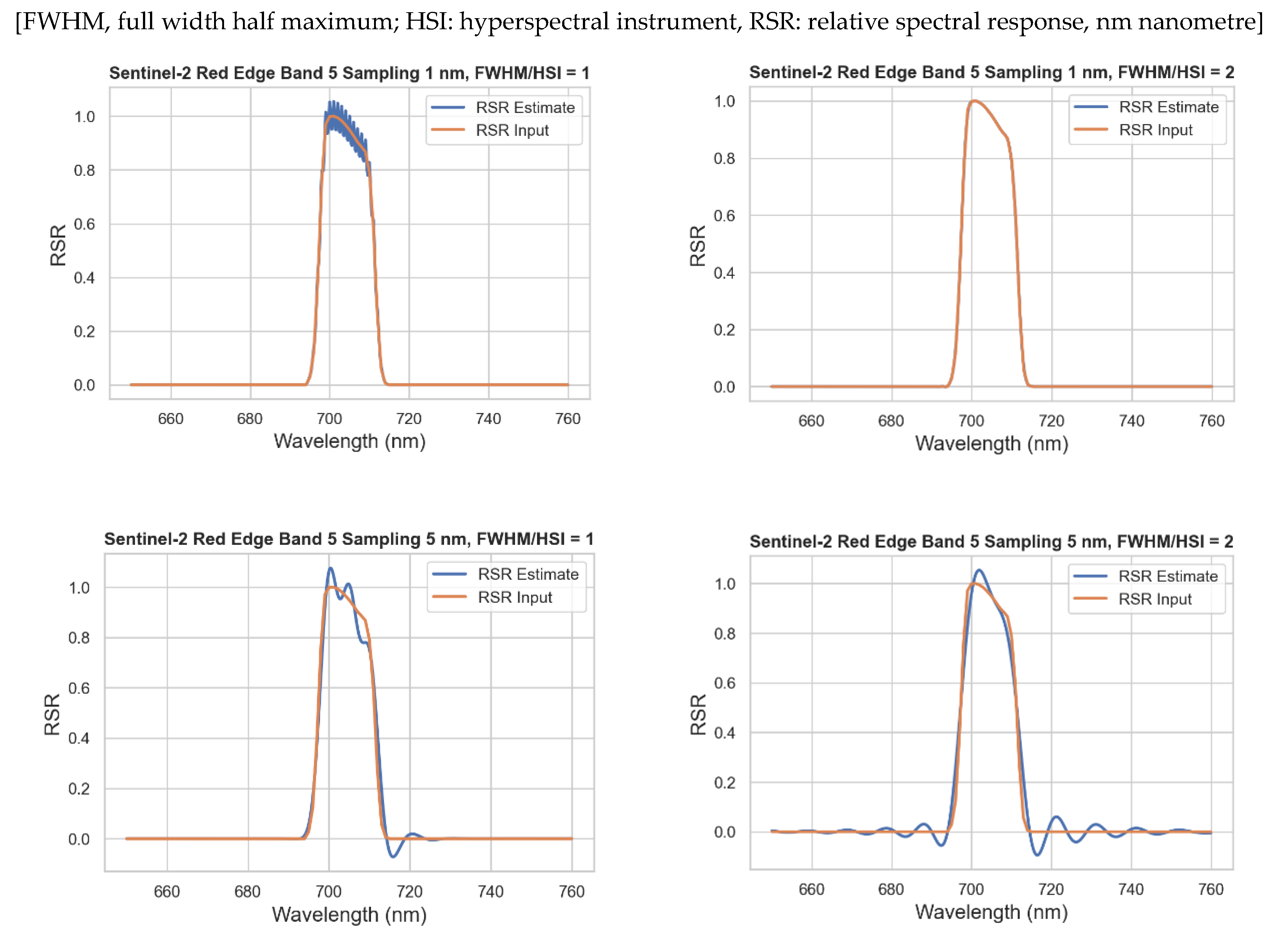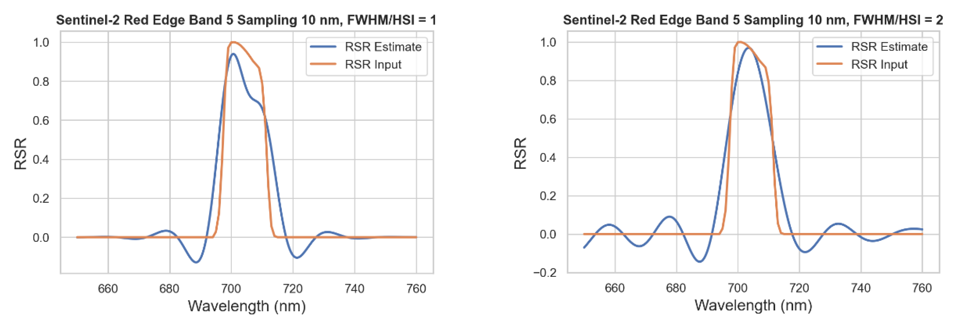Figure 5 illustrates why fine hyperspectral resolution is important for accurate spectral synthesis of multispectral bands. This process of spectral synthesis obviates the need for spectral band adjustment. Figure 5 shows 1, 5, and 10 nm sampling intervals and full width at half maximum (FWHM) values equal to the sampling and twice the sampling. In cases where the FWHM is equal to the sampling interval, the aliasing or ringing is strong. This ringing does not strongly affect the area of the simulated RSRs. When the FWHM is larger than the sampling, the ringing is reduced, and the area under the RSR is conserved. Therefore, a threshold spectral resolution of 1–2 times the spectral sampling interval is proposed for the SCR. Instruments like CLARREO Pathfinder and TRUTHs have the spectral resolution FWHM as twice the sampling to avoid aliasing. The simulations showed that FWHM should be greater than the sampling interval to avoid severe aliasing and can be larger than 2 times the sampling interval while not substantially affecting the RSR simulation. Note that for practical purposes, a 1 nm sampling interval has a negligible error due to the high sampling density, and in this case, the FWHM is equal to 2 nm; hence, the plots overlay one another.

3.3. Radiometric Requirements

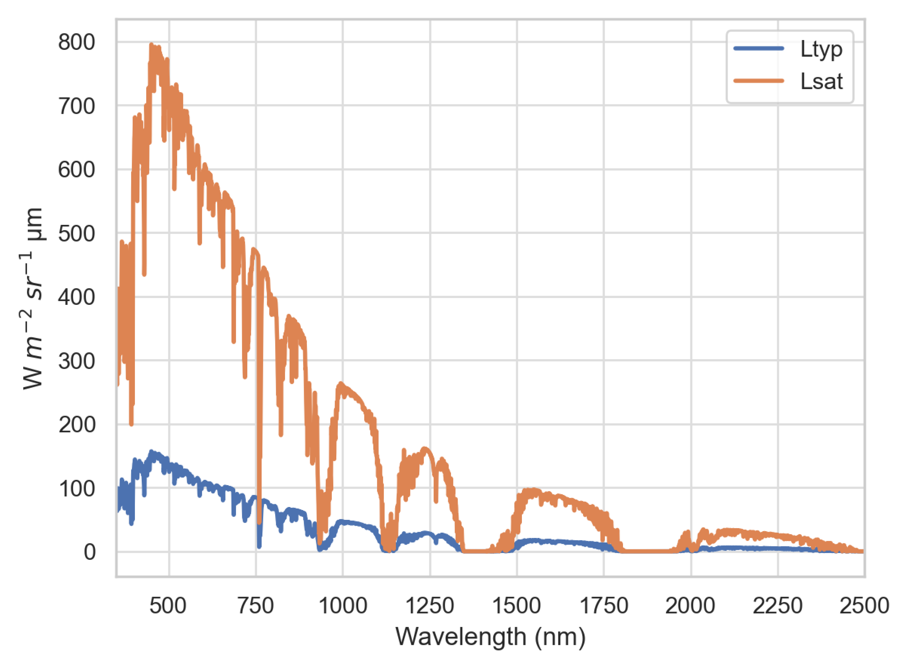
Due to the synoptic coverage achievable over a range of land cover targets, the SCR should be able to operate over a wide dynamic range, including bright targets such as clouds near the equator and low solar elevation dark targets near the poles. The Ltyp is defined as the typical spectral radiance based on a MODTRAN 6 radiative transport model [24] for a 45° solar zenith angle, a 30% albedo surface, the Mid-latitude summer atmosphere (MLS) and rural aerosol with a 23 km visibility. Ltyp is used to define the baseline radiance. Figure 6 shows the Ltyp and Lsat profiles used to estimate the baseline radiance. Ltyp represents a relatively bright radiance (e.g., desert), and Lsat is defined to be slightly brighter than a Deep Convective Cloud (DCC). DCCs are near-Lambertian solar reflectors that are often found above tropical regions. These are good candidates for calibration because they are bright targets located at altitudes where the impact of the atmospheric water vapor and aerosols is low and have been found useful for vicarious calibration in the visible near-infrared (VNIR) region [25,26].

DCCs are approximately an order of magnitude brighter than Ltyp; therefore, the saturation radiance (Lsat) was set slightly higher than the value for DCC. Using MODTRAN, the saturation radiance was defined to be 1.15 times the radiance of a 100% Lambertian target at a 10 km altitude and 0° solar zenith angle. A variable exposure may be needed to operate over this wide dynamic range, as outlined in the nominal instrument specifications in Table 4.

3.3.1. Radiometric Accuracy

The SCR could enable many remote sensing applications by improving SI calibration uncertainties to within 3–5% [27] and the uncertainties of relative calibrations to a reference mission or the transfer calibration uncertainty (TCU) to no more than 1%. The SCR would rely heavily on vicarious calibrations using cross-calibration, field campaigns, Pseudo-Invariant Calibration Sites (PICS), RadCalNet, and DCCs. These calibrations would form the basis for the absolute radiometric SI traceability, flat-fielding, and RSR. Although these methods are typically capable of 3–5% [28] uncertainties, recent work indicates lower uncertainties could be possible [29].

3.3.2. Transfer Calibration Uncertainty

As a transfer radiometer, the SCR will be tied to a reference instrument, such as Landsat or Sentinel-2. After a series of cross-calibrations and careful selection of scenes with minimal cloud cover, near SNOs appropriate to instrument parameters (Table 4), and characterisation, it is expected that the TCU ($u_t$) between the reference instrument and the SCR should be better than 1%. This assumes that the SCR instrument has excellent stability and will not drift over cross-calibration time duration. A TCU cross-calibration period requirement of 1% drives several of the instrument requirements listed in Table 4. The uncertainties include systematic $u_{syst}$ and random components $u_{rand}$ and can be combined as follows:

$$u_t=\sqrt{u_{syst}^2+u_{rand}^2}$$

The systematic components include calibration errors for the flat fielding, linearity, spectral, and spatial stray light. Other components include spectral synthesis and polarisation. These errors can be kept below 1% with careful instrument design (e.g., fine spectral sampling, resolution, radiometric stability; refer to Table 4 and Figure 5), characterisations, and operational considerations. The random component includes atmospheric drift, BRDF effects due to differences in solar and viewing geometries, spatial misregistration between the SCR, and unmodeled polarisation errors. The random component assumes that measurements are uncorrelated between collects. The random component uncertainty can be reduced by the square root of the number of collects $N_{collects}$. A collect is a single independent SNO.

$$u_{rand}=\frac{{\overline{u}}_{rand}}{\sqrt{N_{collects}}}$$

The ${\overline{u}}_{rand}$ is an average random uncertainty that will depend partially on the SNO time differences, landcover selection, and BRDF. The SCR transfer calibration uncertainty was estimated as a function of the number of cross-calibrations performed.

Recent cross-calibrations [30] between Landsat 8 and Landsat 9 OLI instruments show that the TCU can be less than 1% if several potential error contributors are accounted for. While these cross-calibrations were not used to develop a new SI traceability, they were used to understand the relative gain differences between Landsat 8 and 9 for each spectral band. While Landsat 8 and Landsat 9 are nearly identical instruments, the SCR hyperspectral instrument allows for near-perfect RSR matching, so the methodology and conclusions of this work can be extended to SNOs. This work showed that the largest contributor to the OLI TCU was the BRDF differences, and for a 7.5 degree, it could be as large as 10%. Still, a linear model as a function of View Zenith Angle differences was developed, and the intercept of this model was used to determine the gain ratio. This correction reduced the overall TCU to approximately 0.5% in most cases. This work analysed the Ross-Li MODIS BRDF [31,32] model developed for coarser resolution data sets. It is expected that the SCR could have spatial resolutions larger than 30 m, which would be more appropriate for this model, and direct use of the Ross-Li BRDF model could be possible. For the SCR, we expect that the spectral data would be used to classify the landcover, and a BRDF correction would be made for a few landcover types, such as barren or vegetation, as was performed for the Landsat cross-calibration work.

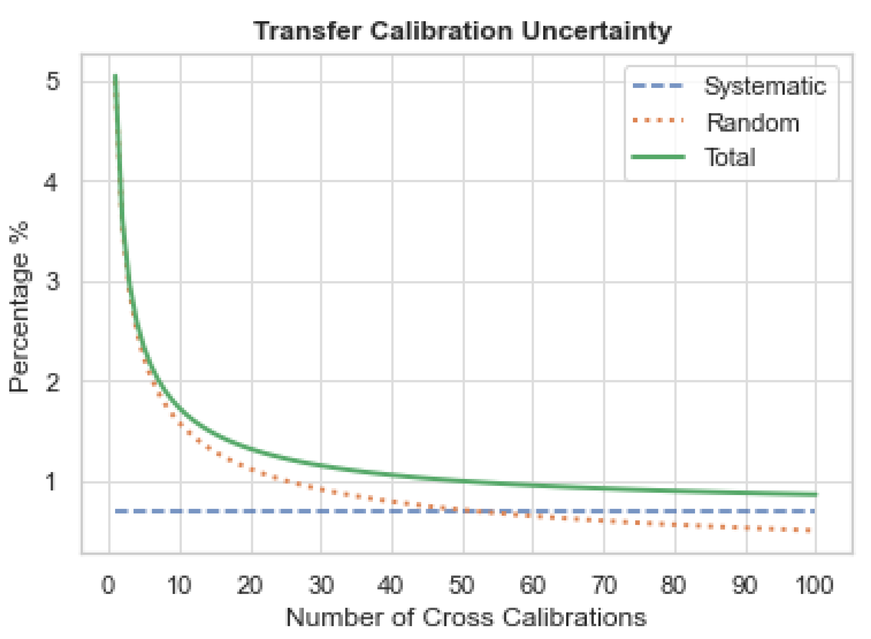
Figure 7 shows that the TCU converges towards 1% as the number of cross-calibrations increases. Three curves are depicted: the first shows the systematic uncertainty error; the second shows the average random uncertainty error; and the third shows the total error. In this case, the systematic uncertainty error is 0.6% and the average random uncertainty is set to a very conservative 5%. One would expect that, with a careful selection of scenes (e.g., SNOs, low cloud cover, and, if possible, Lambertian land cover), this parameter would be a few percentage points less. The figure of 5% was selected because it represents the upper limit of typical vicarious calibration. Even with these conservative values, after ~50 independent collects, the TCU will be less than 1%. Also note that although this may be many collects, many SNOs can be near the poles, and PIC sites will have lower uncertainties.

Having an onboard calibrator to assess stability and provide SI traceability is ideal. However, an onboard calibrator may not be able to be accommodated on the SCR due to cost or complexity constraints. As a result, prelaunch characterisation and in-orbit vicarious calibration would be critical. Without an onboard calibrator, the radiometric stability requirement has been set at less than 0.2% over seven days or better. The value of 0.2% over 7 days has been chosen because a prelaunch characterisation could be performed in a week.

For the threshold values considered, the TCU will decrease to be less than 1% after ~35 collects for near-coincident collects and much faster for near-SNO data collects.

The SCR is likely to have an instrument polarisation sensitivity an order of magnitude higher than that of CLARREO Pathfinder, TRUTHS, and LIBRA, which are designed to have polarisation sensitivities of less than 0.5%. Strategies to mitigate the impact of scene polarisation warrant consideration.

3.3.3. Signal-to-Noise Ratio

The SCR SNR thresholds at the defined typical radiance (Ltyp) and 10 nm full width half maximum (FWHM) spectral width equivalents are referenced in Table 4. Its SNR for a 10 nm spectral resolution equivalent (after aggregation or spectral synthesis of hyperspectral data) exceeds the values for the spectral regions defined in Table 4, which are comparable to EO-1 Hyperion and higher than early CLARREO Pathfinder SNR goals. SNR for CLARREO Pathfinder was as low as 20–33 when measured at a solar zenith angle of 75° and 30% albedo, conditions comparable to the measurement of Ltyp [11].

Although a larger number of samples reduces uncertainty, most real-world scenes have large spatial variations. Other studies have shown that simple regression or averaging the number of samples available in cross-calibration even with SNRs like CLARREO Pathfinder can achieve less than 1% gain uncertainties [16]. Limiting selections within these scenes to extremely uniform areas could substantially reduce the number of usable spatial samples and cross-calibration opportunities. Using linear regression to estimate the gain or offset could provide an alternative to using only uniform scenes. This approach could also identify non-linearities and provide calibrations using typical scene radiance levels. The DESIS and Landsat simulations showed that tens of thousands or more samples can be extracted within an image that has approximately half that of the SCR’s swath dimensions.

3.4. Orbital Characteristics

The primary mission objective of the SCR depends on near-simultaneous nadir observations (SNOs), which are observations of the same areas on the Earth taken at nearly the same time, generally within ±20 min, to minimise the impact of changing sun angle and atmospheric conditions. As most land remote sensing satellites are in sun-synchronous orbits (SSOs), the SCR would also need to fly an SSO. To maximise the amount of land area imaged and thus increase potential SNOs with satellites in any orbit, the SCR orbit was chosen to allow synoptic coverage of the Earth’s land mass within its inclination.

The spacecraft would need to operate in an inclined SSO to satisfy a basic science requirement to acquire imagery under constant solar illumination. The selected orbit would have a nadir repeating ground track with a 48-day revisit period. The satellite orbit would also provide near-simultaneous sunlit overpasses with reference and client satellite missions.

Several orbits were studied to maximise the number and duration of near-simultaneous overpasses between the SCR spacecraft and Landsat 8 and 9, Sentinel-2, and a single Planet Dove. An orbit of 645 km altitude, 97.75 degree inclination, 96.54 min period, ±2.9 degrees FOV, and 10:20 a.m. equatorial crossing time descending mode was selected as the preferred orbit to provide daily averages of the following:

• 16 Landsat 8 and 9 overpasses covering 729,000 square km.
• 14 Sentinel-2a/2b overpasses covering 980,000 square km.
• 4 Single Planet Flock-3p Dove overpasses covering 100,000 square km.

A 48-day repeating nadir SSO works well with system specifications for synoptic coverage and provides a repeat cycle that is harmonic with Landsat, one of the primary reference satellites. This provides consistent, repeating SNO locations and facilitates planning and preparation with the most often-used reference systems.

There are multiple altitudes where a properly inclined orbit generates a 48-day repeating SSO. Several were excluded due to proximity to the busy zones of the communication mega constellations of Starlink (540–570 km) and Kuiper (590–630 km). An orbit at 645 km altitude would provide separation from the mega-constellations as well as enough difference in orbital periodicity to allow for regular SNOs with Landsat.

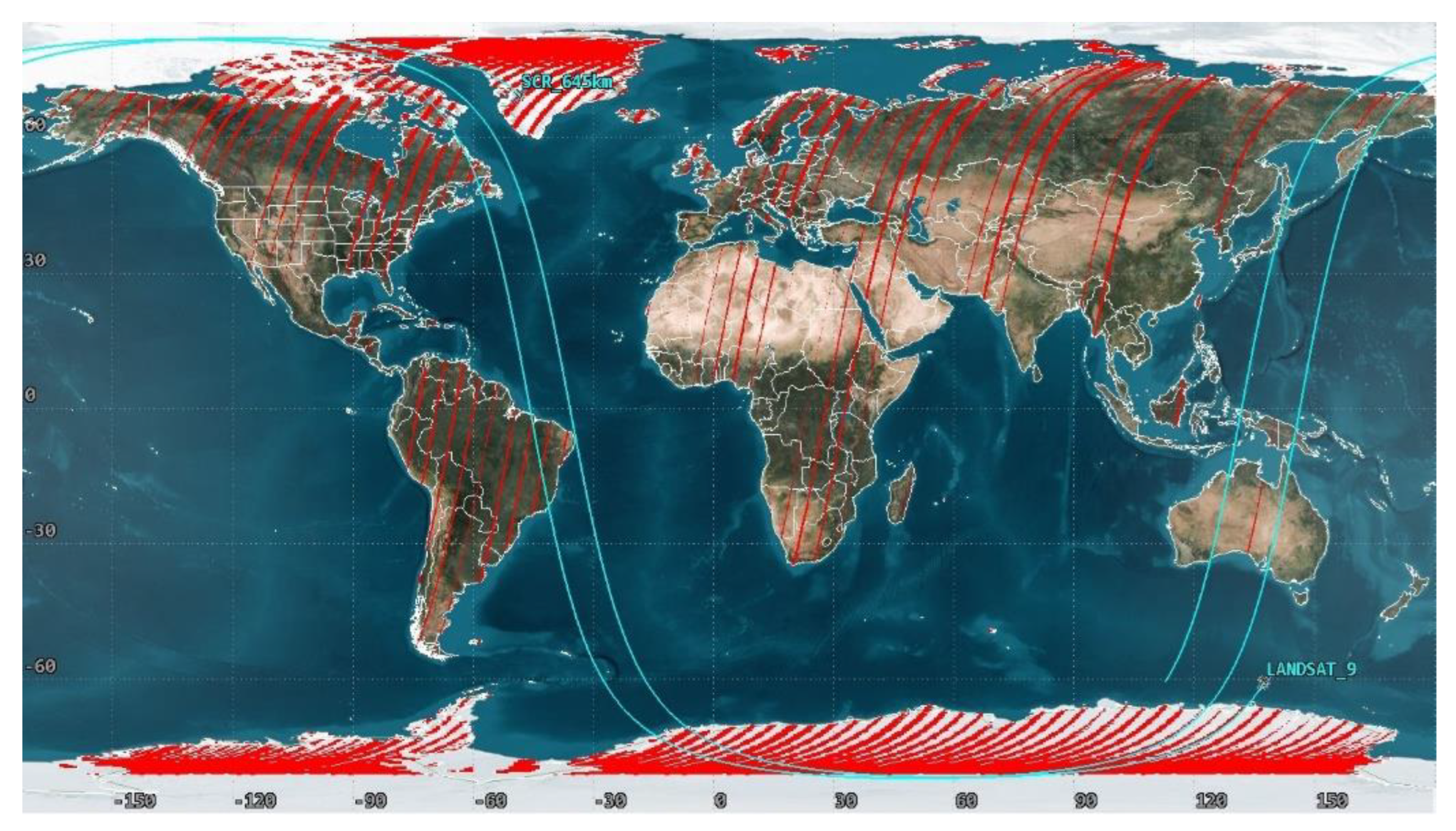
The mean local time (MLT) of equatorial crossing is important to maximise the SNO opportunities between the SCR and reference/client EO missions. The SCR’s intersections with a single Landsat satellite are illustrated in Figure 8. The red areas correspond to the SNO areas over land areas that will be imaged within ±20 min by both Landsat and the SCR. Figure 8 was generated using only the centre ±3° (~75 km) of the Landsat swath to minimise look angle differences that may give rise to BRDF issues.

To capture the SNOs equally across all latitudes as shown in Figure 8, the MLT difference between the SCR and the reference satellite should be minimal, ideally less than 20 min. Hence, the MLT of the SCR was chosen to be around 10.20 a.m. at the descending node for the orbit to be parked between Landsat (~10:00 a.m.) and Sentinel (~10:30 a.m.) orbits to maximise the opportunities between these reference missions.

4. SCR Instrument Calibration

Radiometric calibration is a pre-requisite for creating precise science data and higher-level image products. The SCR instrument is expected to undergo a thorough laboratory-based characterisation during the assembly, integration, and test phase to provide the baselines of the instrument before launch. In a state-of-the-art sensor characterisation laboratory such as the Goddard Laser for Absolute Measurement of Radiance (GLAMR) Facility, absolute radiometric calibration with an uncertainty of <0.09% in the visible and 0.3 to 1% uncertainty in other spectral regions can be achieved [33]. After launch, an extensive in-orbit characterisation will have to take place to measure any performance changes and update the parameters, as necessary. Ongoing calibrations are expected to be performed routinely during the post-launch phases of the mission, including techniques described in [34]. It is expected to include vicarious calibration with automated ground calibration sites, such as the RadCalNet sites, and imaging of PICS to monitor calibration drift over time.

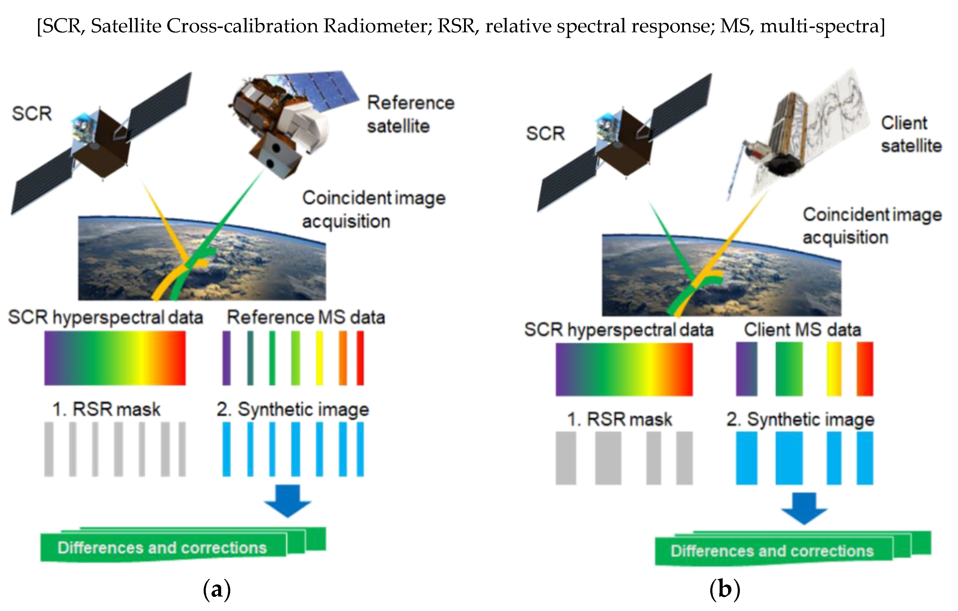
The steps illustrated below apply to the transfer of calibration of the reference system to the SCR. However, these steps apply equally well to the transfer of calibration from the SCR to the client system.

The radiometric characterisation and calibration activities required to achieve calibration transfer include the following steps:

• Perform wavelength calibration using lasers, monochromators, and/or atomic commission lines.
• Measure the spectral response function of the spectrometer channels in the laboratory with a monochromator and/or tuneable laser.
• Determine out-of-band responses (spectral response function and scene generation); include full field of view, spectral “smile”, and keystone evaluation (spectral wavelength calibration).
• Determine radiometric calibration performance, including the absolute (i.e., SI-traceable) and relative radiometry and all artifacts affecting the radiometric accuracy of the data (including linearity, saturation and flat fielding, dark frame characterisations).
• Determine SNR for Ltyp for both VNIR and SWIR wavelengths (i.e., Photon Transfer Curves).
• Measure polarisation sensitivity of the full instrument (i.e., foreoptics and spectrometer) in the laboratory; correct for artifacts in-orbit (polarisation).
• Evaluate VNIR and SWIR spatial performance in the laboratory. (e.g., in-laboratory modulation transfer function (MTF) using knife-edge, line source, or point source illuminated by a monochromator or other narrow-band light source).
• Measure instrument’s geometric distortion using broadband point source or equivalent at various locations.
• Determine corrections to the band location field angles for both VNIR and SWIR (spectral and spatial co-alignment).

The main objective of the SCR is to transfer calibration from the reference sensor to the client sensor, compared to an SITSat which is designed primarily for high accuracy climate monitoring, with the ability to perform in-orbit calibrations accurately. SITSats such as CLARREO Pathfinder and TRUTHS are expected to have SI-traceable radiometric uncertainties well below 1%, which would place them in a league of their own.

5. Notional SCR System Architecture

A notional SCR mission architecture would consist of three main segments: the space segment, launch services segment, and the ground segment. The space segment is represented by the SCR, which would be composed of the spacecraft host bus, and the hyperspectral instrument. The launch segment would consist of the launch vehicle services to place the SCR in orbit, and the ground segment would consist of the science data processing system. A schematic representation of the notional SCR mission segments is illustrated in Figure 9.

6. Discussion

The SCR instrument requirements described in this paper are based on fulfilling the primary goal of the SCR mission, which is to enable cross-calibration and comparison of commercial EO missions with highly calibrated missions, such as Landsat and Sentinel-2, and reduce radiometric uncertainties of surface reflectance data products generated by the missions. The SCR instrument would be a hyperspectral imaging spectrometer that collects data in the visible and near-/shortwave-infrared portions of the spectrum (400–2500 nm) to generate data in narrow spectral bands spaced less than 5 nm apart in the visible region (400–900 nm) and less than 10 nm in the near- and shortwave-infrared region (900–2500 nm). The spectral channel resolution is designed to be 1.0 to 4.0 times the channel spacing to avoid spectral aliasing. With the exception of extremely narrow bands, the spectral sampling selected will introduce no more than 1% uncertainty to the predicted TOA spectral reflectance for cross-calibration operations [35]. It is highly likely that power, mass, and volume constraints on smaller commercial satellites would limit the use of onboard sensor calibration equipment. An SCR instrument in orbit through its role as a calibration transfer radiometer could therefore address shortcomings related to onboard calibration on commercial systems.

A consistent ground track is required for periodic cross-calibration collections and other mission planning purposes, as well as to maintain imagery characteristics over time and to ensure global data acquisition without gaps. The SCR overpasses need to be under sunlit conditions and evenly spread across the globe to increase the chances of coincidence with reference and client satellite systems.

A study on user requirements for moderate-resolution land imaging by future Landsat satellites identified a need for increased spatial, spectral, and temporal resolution for the reflective and thermal infrared bands [14]. The user requirements for enhanced resolution can also be seen to be expressed in sensor specifications for future commercial missions. This implies a need for better consistency and quality of data expected from a multitude of missions for their synergistic use.

The SCR user community is initially expected to include calibration/validation engineers and scientists representing government and commercial client satellite systems. As a primary objective, users would have access to the same tools and calibration information as the SCR calibration/validation team. Global satellite orbit information that is publicly available online, or through specific tools developed for the SCR mission, would provide the location and times for coincident cross-calibration data collects. The aim would be to provide open access to data, information, and tools to help the growing EO community to improve the calibration of instruments that generate data. Using SNOs, users would be able to cross-calibrate the SCR and reference or client systems. They can create synthetic images and compare synthetic images with the client or reference system to perform cross-calibration. The resulting spectral/radiometric differences and corrections can then be used to update client system calibration and can be made available to the calibration/validation community. Additionally, an archive of hyperspectral imagery collected by the SCR could provide a rich EO data resource for scientific analysis and applications and an evidence base that informs the need for future missions.

Translating the SCR concept into operational reality depends on several factors: Securing a COTS hyperspectral instrument that satisfies the nominal sensor requirements for the SCR without too many compromises will be critical. Rigorous screening procedures on the ground to ensure that the chosen instrument meets the requirements of the SCR before launch are important. Also, securing appropriate launch services to achieve the precise orbit, alongside cooperative client satellite operators that share sensor characteristics/parameters (e.g., spectral response functions) to achieve accurate spectral synthesis and are open to updating the calibration on their satellites based on SCR outputs, will be critical to deliver the expected benefits.

7. Conclusions

This paper presented the concept of a satellite Cross-calibration Radiometer for transferring the TOA radiance from an in-orbit reference or benchmark satellite to a client satellite through spectral synthesis to improve its data quality and interoperability. The benefit to the users is the improvement in uncertainties in the TOA radiances in the commercial optical satellites to bring these closer to those highly calibrated optical satellites, which are calibration reference standards. This could result in overall improvements to data quality across multiple sensors.

The SCR requirements were developed using simulations and sensor performance trade-offs to quantify the impact of key sensor parameters on cross-calibration. Simulations have shown that the SCR could achieve transfer calibration uncertainty values of no more than 1% through multiple cross-calibration opportunities with reference and client satellite systems, which would enable effective in-orbit transfer of TOA radiance. Through the process of cross-calibration, the radiometric accuracy of optical EO data could improve from 5% to 3%. In conjunction with transfer calibration that is stable to a fraction of a percent, it would be possible to improve the quality of optical EO data to better support climate change modelling and ecosystem monitoring applications.

Consequently, improved surface reflectance products and a higher radiometric accuracy of calibrated observations at TOA could result in improved downstream data products as a result of this transfer from the reference system to the client satellite system. Furthermore, this could enable the data harmonisation or interoperability of the virtual constellation.

Establishing a space-based Cross-calibration Radiometer would enhance the interoperability of historical and future sensor datasets and improve the accuracy and reliability of EO data. Further, the SCR could make a unique contribution to improving the utilisation of global EO data in a way consistent with efforts by the Committee on Earth Observation Satellites (CEOS) and Group on Earth Observations (GEO).