Article

Intelligent Detection and Segmentation of Space-Borne SAR Radio Frequency Interference

1
National Key Laboratory of Radar Signal Processing, Xidian University, Xi’an 710071, China
2
Air Force Early Warning Academy, Wuhan 430019, China
3
Hangzhou Insititude of Technology, Xidian University, Hangzhou 311231, China
*
Author to whom correspondence should be addressed.
Remote Sens. 2023, 15(23), 5462; https://doi.org/10.3390/rs15235462
Submission received: 10 September 2023 / Revised: 17 November 2023 / Accepted: 20 November 2023 / Published: 22 November 2023
(This article belongs to the Special Issue SAR Data Processing and Applications Based on Machine Learning Method)

Abstract

:
Space-borne synthetic aperture radar (SAR), as an all-weather observation sensor, is an important means in modern information electronic warfare. Since SAR is a broadband active radar system, radio frequency interference (RFI) in the same frequency band will affect the normal observation of the SAR system. Untangling the above problem, this research explores a quick and accurate method for detecting and segmenting RFI-contaminated images. The purpose of the current method is to quickly detect the existence of RFI and to locate it in massive SAR data. Based on deep learning, the method shown in this paper realizes the existence of RFI by determining the presence or absence of interference in the image domain and then performs pixel-level image segmentation on Sentinel-1 RFI-affected quick-look images to locate RFI. Considering the need to quickly detect RFI in massive SAR data, an improved network based on MobileNet is proposed, which replaces some inverted residual blocks in the network with ghost blocks, reducing the number of network parameters and the inference time to 6.1 ms per image. Further, this paper also proposes an improved network called the Smart Interference Segmentation Network (SISNet), which is based on U2Net and replaces the convolution of the VGG blocks in U2Net with a residual convolution and introduces attention mechanisms and a modified RFB module to improve the segmentation mIoU to 87.46% on average. Experiment results and statistical analysis based on the MID dataset and PAIS dataset show that the proposed methods can achieve quicker detection than other CNNs while ensuring a certain accuracy and can significantly improve segmentation performance under the same conditions compared to the original U2Net and other semantic segmentation networks.

Graphical Abstract

1. Introduction

Synthetic aperture radar (SAR), an active microwave remote sensing tool, provides important statistics for observing and comprehending changes taking place on Earth [1]. The high-resolution, all-weather image acquisition capabilities [2,3,4] allow SAR to be applied in a variety of fields, such as earth science, earth system monitoring [1,3,4,5], etc. In recent years, SAR satellites have developed rapidly. There are more than 100 SAR satellite constellations worldwide, and the market value exceeds 10 billion. On the one hand, space-borne SAR is currently focusing on advancing the resolution and swath to a new level. On the other hand, the robustness of SAR needs to be further improved.
Since SAR is a broadband active remote sensing radar system, radio frequency interference (RFI) is one of the biggest challenges and has various forms and sources (see Figure 1); in addition, some non-human factors often affect SAR observations, such as atmospheric [2,3,4,5,6] or boundary noise [7].
At present, with the use of electronic equipment increasing rapidly, the electromagnetic environment is becoming more and more complex. For example, TV broadcast signals, wireless communications, active jamming signals, and other non-cooperative SAR signals interfere with SAR observations. These incoherent electromagnetic signals appear as multiple bright lines or curved stripes in the SAR image domain [8] or appear in the form of dense raindrops as shown by the different colored artifacts in Figure 1, which seriously undermine the performance of SAR observation of the land and sea. In the spirit of ensuring overall data quality, it is imperative to detect and mark the RFI artifacts of SAR images instead of disregarding the RFI-contaminated data [9].
It is well known that any frequency band allocated for remote sensing of the Earth will be affected by RFI. However, due to the higher density of spectrum usage, lower frequency bands may be affected more by RFI. In recent years, L-band radars have reported more RFI interference [10]. In addition, C-band radars [11], such as Sentinel-1 and Gaofen-3 satellites; X-band radars [12], such as Terra-SAR satellites; and K-band radars [13] have all found some signs of RFI, with other, weaker RFIs remaining undetected.
Urged by the demand of an intelligent monitoring system that will automatically mark images with RFI artifacts, this article concentrates on RFI artifact detection and segmentation in C-band Sentinel-1 SAR data. Specifically, this paper aims to solve the problem of serious ill-distribution of positive and negative samples caused by a small number of RFI samples in massive SAR data, as well as the multi-scale problem caused by the multi-modal characteristic of SAR interference, including the size and performance of RFI artifacts. With different forms, an intelligent RFI artifact quick detection and marking method is proposed. Our goal is to quickly screen RFI samples in the images and accurately mark the exact parts of SAR images affected by RFI.
In early practices of RFI detection, researchers mainly used high-order statistical information of the signal to detect RFI. Among them, Antoni, J. proposed the method of using spectral kurtosis [14] to characterize non-stationary RFI signals. Later, Roger, D. et al. used simulated pulse sinusoidal signals to conduct a sensitivity test on the spectrum kurtosis algorithm [15]. In addition, Jarque, C.M. and Bera, A.K. combined the kurtosis and skewness statistics and proposed the JB detection statistic [16], which was later used for outlier detection. Different from previous studies of RFI based on raw data [1,3,10,17,18], our research is conducted on quick-look images of Sentinel-1 single-look complex (SLC) or ground range detected (GRD) data. Work related to interference segmentation on quick-look images has been rarely investigated previously. A few papers have described the segmentation methods of interference through time-series detection [19], image processing [20], and polarization difference [21] but are either poor in robustness or require a large amount of non-interference comparison data, restricting their application. In contrast to the above methods, the proposed methods possess the advantages of low implementation complexity and high robustness and are free from predefining thresholds.
Furthermore, the application of artificial intelligence has been proved by some very successful works recently, paving the way for further research on RFI detection. Yu, J. et al. [4] proposed a single-shot multi-box detector (SSD) method for multi-class RFI detection using rectangular bounding boxes to mark the RFI components in the time–frequency image. Similarly, [22] mentioned a detection method based on Faster R-CNN in the range–doppler domain. By contrast, SISNet achieves RFI segmenting, that is, pixel-level detection, which is more precise. Further, these methods require Fourier transformation of the echo before detection, which increases the data processing dimension and introduces additional calculations. In [23,24], DCNN structures such as VGG and ResNet networks are used for RFI detection. The authors used a binary classification method to distinguish between images with and without interference. According to the comparison test results below, compared to these methods, the IQDN network can detect the presence of interference faster while maintaining similar accuracy.
The research is carried out in the following manners. In the beginning, the interference-targeted quick-detection network (IQDN) is constructed on the basis of the modified MobileNet V2 network, which replaces inverted residual blocks with ghost blocks and adds attention mechanisms at the head of the network to spot the existence of RFI in the quick-look images of the MID dataset according to the difference between an image with RFI and an image without RFI. Then, an improved U2Net called ’SISNet’ is proposed and employed to segment the RFI artifacts in the image domain on the quick-look images of the PAIS dataset.
The following states the main contributions of this paper:
(1) The IQDN algorithm designed upon the modified MobileNet V2 [25] network is proposed, which can effectively detect the existence of RFI in the image domain. It surpasses the cutting-edge algorithms using current convolutional neural networks (CNNs) such as VGG-16, ResNet, and MobileNet in inference time consumption while maintaining a certain accuracy;
(2) An RFI segmentation algorithm designed upon SISNet is built. In contrast to current semantic segmentation networks, the SISNet advances the RFI segmentation performance significantly according to hypothesis testing. Moreover, the SISNet can extract features of the RFI without interference-free comparison images, reducing repetitive work for data collection.
The rest of this paper unfolds as follows. Section 2 elaborates the mechanism of RFI formation and its classification. Section 3 explains the construction of the MID and PAIS datasets and introduces DCNN and semantic segmentation networks. Section 4 elaborates the IQDN algorithm based on the modified MobileNet V2 network and the interference segmentation algorithm named SISNet. Section 5 exhibits the results acquired from the experiments on the IQDN and SISNet; this is followed by the discussion in Section 6 and conclusions in Section 7.

2. RFI Classification and Formulation

2.1. Why RFI Can Affect SAR Observations

The weak links within SAR makes it possible to undermine its performance. First of all, the power capacity of space-borne SAR is limited, so the energy of the reflected echo signal of the ground target is weak. Secondly, SAR cannot form a narrow beam before receiving a predetermined number of pulses, and a wide beam is still active at each unit position of the synthetic aperture. Moreover, the high resolution of the SAR azimuth depends on the principle of the synthetic aperture, and the characteristics of the transmitted signal are generally required to remain unchanged within an aperture time. In addition, SAR imaging uses coherent pulse compression technology, which requires high coherence in the azimuth and range of signals.

2.2. Interference Classification

When SAR emits high-power electromagnetic waves to detect targets, its echo signals are inevitably doped with electromagnetic interference signals of the same frequency band from the surrounding environment. According to the energy source, SAR interference can be divided into two categories: passive interference and active interference (see Figure 2).
Passive interference is generated by the reflection of SAR signals by metallic objects such as chaff and reflective nets. Active interference is the interference generated by external electromagnetic radiation sources, which can be divided into two types: intentional interference and unintentional interference. This article mainly introduces a detection method for active SAR interference. Unintentional interference mainly refers to radio frequency interference caused by communication, television, ground radar, and other operating frequencies within the frequency band of the SAR receiver. Unintentional interference usually does not completely spread over the entire image but exists in the SAR image with the characteristics of a scattered distribution and block aggregation, forming multi-point and local occlusions on the real image. Intentional interference is primarily caused by enemy jammers. Intentional interference can usually achieve high-power suppression of SAR signals and appears as a patch of bright occlusion on the SAR image, and ground targets are completely submerged in it. The existence of interference signals affects the results of SAR image processing and information extraction, thereby reducing the application efficiency of SAR image products.

2.3. Interference Formulation

SAR systems operate by transmitting electromagnetic waves of specific wavelengths and then recording the energy reflected after interacting with distant objects. In a specific receiving time window, the received echo can be expressed as a linear mixture of the target echo, interference, and noise—namely [24]:
x ( k ) = s ( k ) + i ( k ) + n ( k ) ,
where k denotes fast time samples, and s ( k ) , t ( k ) , and n ( k ) denote the target echo, RFI, and thermal noise, respectively.
Being extensively researched, the mathematical model of RFI signals usually can be divided into three categories: namely, the narrow-band signal, pulse signal, and wide-band signal. Several signals are selected below as representative RFI signals that are easily encountered in practice.
  • Continuous-Wave Interference:
    i ( k ) = l = 1 L A l ( k ) · exp ( j 2 π f l k + ϕ l ) ,
  • Chirp-Modulated Interference:
    i ( k ) = l = 1 L A l ( k ) · exp [ j ( 2 π f l k + π g l k 2 ) ] ,
  • Sinusoidal-Modulated Interference:
    i ( k ) = l = 1 L A l ( k ) · exp [ j g l sin ( 2 π f l k + ϕ l ) ] ,
    where A t ( k ) , f l ( k ) , g l , and ϕ i denote the amplitude, frequency, modulation factor, and initial phase, respectively. L represents the number of interfering components.

3. Materials

3.1. Dataset Creation

This paper employs quick-look images of Sentinel-1 Level-1 SLC and GRD products due to their various merits. Firstly, these data are available orderly and free of charge for online downloading. Moreover, they feature a wide swath and high resolution as the Sentinel-1 SAR mainly functions in the interferometric wide (IW) mode over land [27,28]. Last but not least, the quick-look images are colored, lower-resolution versions of the original images. There are three channels in quick-look images, with the red channel (R) representing the co-polarization VV, the green channel (G) is the cross-polarization VH, and the blue channel (B) is the ratio of the cross and co-polarizations. These three channels are mapped to RGB colors to form a pseudo-color image as shown in Figure 3, which provides convenience for direct screening of interference through visual observation in the process of data labeling. The original SLC and GRD products are on the order of several gigabytes, while their quick-look images have a size of tens to hundreds of kilobytes. Considering storage and processing issues, the selection of quick-look images facilitates the creation of datasets and the application of deep learning techniques. Thus, it detects RFI artifacts effectively.

3.1.1. Multi-Scale Interference Detection Dataset

The impact of RFI on SAR determines that RFI’s artifacts in the image after SAR imaging will present characteristics such as being multi-style and multi-scale. With the increasing demand for RFI detection and recognition, it is necessary to construct a multi-scale RFI dataset. For the RFI artifacts studied in this paper, there is no multi-scene, multi-style, and multi-scale RFI artifact image dataset available. Therefore, two new datasets for RFI detection and segmentation, named the ’MID dataset’ and the ’PAIS dataset’, come into being.
The multi-scale interference detection (MID) dataset is set up using 130 quick-looks of SLC products obtained from the official website of the European Space Agency [29]. These RFI-contaminated SAR data are derived from observations of the Korean region by the Sentinel-1 satellites, and the time span ranges from May 2021 to May 2022. The MID dataset contains a variety of polarization modes and a total of about 30,000 slices with multiple resolutions, among which more than 5000 slices are contaminated by RFI.
We carefully select 100 images with strong RFI features. Since 100 images are insufficient for deep learning, we use random cropping on these quick-look images and retain the new images that are large enough in size to expand the dataset. In addition, in view of the multi-scale characteristics of RFI, we crop these images into slices of 256 × 256, 512 × 512, and 1024 × 1024 at a ratio of 4:1:1, and the total number of images is 30,000. Since some of the cropped images are still too large to be applied to CNN, these images are resized to 224 × 224 and are manually divided into two categories: with RFI and RFI-free. This method can change the size of the area contaminated by RFI in the image while using the same quick-look image, which enhances the robustness of the network to multi-scale features. Figure 3 tells that the training data contain a variety of different types of RFI, and there is no need for a one-to-one match between RFI and non-RFI scenes.
As is known, RFI only occupies a small area in the image. In the original two classification sample sets, the distributions of the two types of samples are not equal, as the number of images with RFI is relatively small. Therefore, we perform data augmentation only on the RFI-contaminated sample set in order to increase the number of these samples and balance the numbers of the two types of data. The data augmentation methods are applied at a 1:1:1:1 ratio (i.e., 5× data augmentation) and include flipping, blurring, translating and affiliating. In the data of Sentinel-1, RFI artifacts are always distributed vertical to the along-track direction, so it is unnecessary to augment the data by rotating the pictures. After data augmentation, some problematic data are checked and manually removed. A set of samples after data augmentation is shown in Figure 4.
In the final interference detection dataset, the number of samples with interference is 25,655, and the number of samples without interference is 22,270. Then, the dataset is randomized into training and testing sets at a ratio of 4:1. Descriptive information about the MID dataset is shown in Table 1 below:

3.1.2. Polygonal-Annotated Interference Segmentation Dataset

The polygonal-annotated interference segmentation (PAIS) dataset adopts quick-looks of the GRD product corresponding to the SLC products of the MID dataset. The GRD images do not contain phase information and have reduced speckles due to multi-look processing. The dataset contains multiple polarization modes and has the characteristics of various types of RFI artifacts and scenes.
Figure 5 presents some of the augmented data samples of the PAIS dataset shown from left to right in columns. These samples are adjusted from 130 quick-look images that are resized to 572 × 572 as the standard input size and then augmented to 2000 images via flipping, translating, noise-adding, and blurring operations. The data augmentation methods are applied at a 1:1:1:1 ratio. Furthermore, 100 more scenes of GRD products are selected from Sentinel-1’s SAR observation data of other areas.
The RFI-affected areas vary in number and size in each image. It takes days for us to use the Labelme 5.0.1 software to manually label the location of the interference in the image to form a semantic segmentation mask using the polygonal-annotated method and to save it as a JSON file. There are more than 4700 instances of RFI artifacts, covering a variety of styles and sizes. Then, we use the JSON files to generate the corresponding one-channel label images, modify the label images and the original images to have the same file names, match the image to the label, and store the files in two folders. Similarly, the data are randomly divided into a training set and validation set at a ratio of 9:1 during training. In summary, the PAIS dataset consists of six folders, including JPEGImages, Annotations, SegmentationClassPNG, TestImages, and TestSegmentationPNG. In these folders, JPEGImages contains 2000 images used for training and validating, while the Annotations and SegmentationClassPNG folders are the corresponding JSON annotation files and segmented label images, respectively. In the same way, the TestImages and TestSegmentationPNG folders consist of test images and their label images, respectively. Samples of the PAIS dataset are show in Figure 6:
Information about the PAIS dataset is shown in Table 2 below:
The ground range coordinates of the GRD products are the slant range coordinates projected onto the ellipsoid of the earth, which means GRD data can be related to geographic information. In a sense, the location of RFI can be realized by segmenting the RFI of GRD data.

3.2. Deep Neural Network

A deep convolutional neural network (DCNN) is a feedforward network whose artificial neurons can respond to surrounding units; they have been proved effective in multiple fields such as image classification [30,31,32], target detection [33,34,35], semantic segmentation [36,37,38], etc. VGG network, proposed by Simonyan et al., achieved astonishing classification results [27]. ResNet was born in 2015 and has a top error rate of 3.57%. ResNet [30] proposes residual skip connections between layers, introduces forward information, alleviates gradient disappearance, and makes it possible to deepen neural networks. MobileNets [39] are lightweight DCNNs using depth-wise separable convolutions for mobile and embedded vision applications. The network properly balances latency and accuracy by introducing a width multiplier and a resolution multiplier. Motivated by these lines of work, we take in the capacities of deep learning to determine whether the SAR images are contaminated.
The basic module of a CNN is composed of input and output layers and multiple hidden layers. The hidden layers consist of convolutional layers, pooling layers, activation layers, and loss layers.

3.3. Semantic Segmentation Network

Semantic segmentation distributes semantic categories to pixels of the input image to obtain pixel-level classification. Since 2015, intelligent image segmentation methods have been extensively applied in bio-medicine [40]. A common semantic segmentation framework is an encoder–decoder network: (1) Encoder: usually a pre-trained classification network, such as VGG [27], ResNet [30], or other deep neural network; (2) Decoder: the decoder semantically projects the discriminative features (lower resolution) to the pixel space (higher resolution) to obtain pixel-level classification.
Under this structure, we down-sample the spatial resolution of the input image to develop low-resolution feature maps that can efficiently classify object classes. The feature representation is then up-sampled to form a full-resolution segmentation map. Semantic segmentation requires not only discriminative capabilities at the pixel level but also a mechanism that can project the discriminative features at different stages to the pixel space [41] (i.e., map back to the original image size). Different architectures employ different mechanisms (skip connections, pyramid pooling [42], etc.) as part of the decoding mechanism.

3.3.1. FCN

In November 2014, Long et al. designed an end-to-end, pixel-to-pixel semantic segmentation method using a fully convolution network (FCN) [43] (see Figure 7). The authors of the paper proposed to improve an existing and well-researched image classification model (such as AlexNet [44] or VGG). They applied their method to the encoder module of the semantic segmentation network and added a decoder module with a transposed convolution layer to realize coarse feature maps that were up-sampled to obtain full-resolution segmentation maps.
The FCN model structures include FCN32s, FCN16s, FCN8s [36], and other structures according to the fine-grained segmentation. FCN32s restores the feature map from a 32-time down-sampling size to the input size, and FCN16s and FCN8s, respectively, restore it from a 16-time and 8-time down-sampling size to the input size. The smaller the number, the more up-sampling operation deconvolution layers used, the more complex the corresponding model structure is, and the finer the segmentation effect is in theory. The schematic diagram of an FCN network is shown as follows:

3.3.2. UNet

A new semantic segmentation network called UNet was proposed by Ronneberger et al. [45] (see Figure 8) in 2015, which improved the fully convolution structure mainly by expanding the decoder capacity in the network. Specifically, the authors proposed a U-shaped network structure to capture context and achieve accurate localization. This simpler structure has become very popular and has been applied to various segmentation practices.
The standard U-Net model consists of a series of convolution operations at each block in the network. Instead of stacking convolutional layers, there are many higher-level blocks that can be stacked to build a network structure. Using this idea, researchers successively proposed Recurrent Residual UNet [46], Attention UNet [47], UNet++ [48], U2Net [49], and other networks.

3.3.3. U2Net

Over the years, we have seen auto-encoder models like Deeplab [50] used for semantic segmentation. Among all segmentation models, there is still a name that is at the top of the list: U-Net. U-Net was released in 2015. Since then, it has gained enormous popularity and is used for several different tasks related to segmentation. A variant of U-Net called U2-Net [49] was released in 2020. Basically, U2-Net is composed of two U-Nets.

4. Methodology

Here, the training process and network frameworks of the proposed IQDN and SISNet are laid out. Then we elaborate on the metrics for evaluating performance.

4.1. Interference-Targeted Quick-Detection Network

An important step in recognizing and mitigating radio frequency interference is to determine the existence of interference in the SAR data. To judge for the existence of RFI, we can intuitively observe from the SAR image. If there are bright lines or block artifacts in the image, it can be considered that there are RFI artifacts in the data. However, SAR satellites can generate a large amount of SAR data every moment, and it is time-consuming and labor-intensive to screen SAR data through manual discrimination. Therefore, we attempted to realize intelligent discrimination by training a neural network to replace the manual work.
Using the classic convolutional neural network model to classify and recognize images has problems such as a large number of parameters, a large amount of calculations, a large model, and high equipment requirements. Previously, Weiwei fan et al. [24] realized RFI detection based on time–frequency domain images by applying a VGG network. However, the number of VGG network parameters is as high as 138 million, which severely limits its inference speed. In the face of massive SAR data, the speed of screening interference data is particularly important. The MobileNet V2 [25] network is a lightweight, deep convolutional neural network proposed by Google for intelligent embedded devices. The core of the network is the combination of depth-wise separable convolution and an inverted residual block, which achieves better performance with a smaller amount of computation. But it still meets the problem of low recognition accuracy and large prediction errors.
Aiming to solve these problems, a modified MobileNet V2 called ’IQDN’ is proposed, the framework for which is shown in Figure 9. Firstly, by integrating the spatial and channel attention mechanism [51] (convolutional block attention module (CBAM)), the network model can enhance the refinement ability of the interference features and reduce the impact of irrelevant features. Secondly, we replace the part of convolution module with a ghost module, reducing the number of parameters while ensuring accuracy, and finally, we replace the ReLU6 activation function in the depth separable convolution module with LeakyReLU to retain more positive and negative feature information in the image.
The idea of the attention mechanism comes from the human visual attention process, and attention focus is added to the key area to obtain the required details. CBAM [51] is an attention module that includes a channel attention module and a spatial attention module so that the model can simultaneously carry on channel calibration and spatial calibration. However, the fully connected layer and convolution kernel with a large receptive field will greatly increase the parameter number of the module. In the improved model proposed in this paper, by introducing a lightweight channel and spatial attention module (LCBAM), the design uses a one-dimensional convolution operation to aggregate channel features for one-dimensional channel attention and uses dilated convolution with a kernel size of 3 × 3 in two-dimensional spatial attention to aggregate spatial features, which minimizes the number of module parameters while better obtaining interference features. Considering that the deep layer of the convolutional neural network extracts features such as shape and semantics, we propose a modified MobileNet V2 wherein the LCBAM module is added between the last inverted residual module and the average pooling layer in order to improve the feature extraction ability. The channel attention and spatial attention modules of the mentioned LCBAM module can be expressed by:
M C ( x ) = σ f 1 D n ( AvgPool ( x ) ) + f 1 D n ( MaxPool ( x ) ) ,
M S ( x ) = σ f dilation 3 × 3 ( [ AvgPool ( x ) ; MaxPool ( x ) ] ) ,
where M c ( x ) is the output of the channel attention module, M s ( x ) is the output of the spatial attention module, σ ( · ) is the activation function, and f 1 D n ( · ) and f d i l a t i o n 3 × 3 ( · ) denote a one-dimensional convolution operation and dilated convolution, respectively, with a kernel size of 3 × 3 .
The ghost module was proposed by Kai Han et al. in 2020 [52]. It is mentioned in the article that although MobileNet or ShuffleNet were proposed to use depth-wise or shuffle operations, the introduced 1 × 1 convolution would still generate a certain amount of calculation, but the authors found when analyzing the output feature map that some feature maps were actually similar. So it is considered that similar feature maps can be obtained by simple transformation: that is, linear transformation. In the ghost module, for a certain feature layer, only a part of the real feature layer (real feature layer) is generated by the convolution operation, and the remaining feature layer (ghost feature layer) is obtained by performing a linear operation on the real feature layer; then, the real feature layer and ghost feature layer are spliced together to form a complete feature layer, as shown in Figure 10:
The compression ratio of the computational cost of the ghost module is proportional to the number of feature maps participating in the linear transformation.
The IQDN is trained on an NVIDIA GeForce RTX 3060 GPU with 12 GB memory using PyTorch [53]. Guided by the Adam solver, IQDN optimizes the parameters. The batch size is 64, the learning rate is 0.01 and descends with a step-wise strategy, and the momentum is 0.9.

4.2. SISNet Structure

In the medical field, since the ultimate goal of medical imaging is to assist doctors in clinical diagnosis, it is far from enough for the network to tell doctors whether a patient is sick from a 3D CT. The doctor still wants to know which layer and where the lesion is located. Similarly, in the field of RFI detection, knowing whether there is interference in the SAR image is only the first step in the cognition of RFI. We also need to know the location of the RFI: that is, which burst the RFI is in on the Sentinel-1 satellite SAR image. Therefore, this paper also aims to use an image segmentation method on the quick-look images of Sentinel-1 SAR data to realize the positioning of RFI.
Here we propose an improved U2Net called SISNet. SISNet replaces the pooling layer and loss function used by the U2Net network to adapt to the pixel-level segmentation task for RFI. Then, a modified receptive field module is introduced to replace part of the dilated convolution layer of the U2Net bottom layers to effectively increase the receptive field and the feature extraction ability of the network. In addition, a lightweight CBAM module is added at the connection of each layer of the encoder–decoder to focus on the key information in the feature map. Moreover, before outputting the predicted mask results, we also introduce a channel attention module to assign weights among the predicted masks output by each layer. Finally, the two-dimensional convolution in the RSU module is replaced by a residual convolution to prevent network degradation.
In 2019, Richard Zhang [54] found that CNN is not translation invariant because when the input is slightly translated or transformed, the output changes dramatically. Richard Zhang believed that this is caused by operations with down-sampling (such as convolution with s t r i d e > 2 and pooling), as these down-sampling methods ignore common sense in the field of signal processing: before the signal is down-sampled, low-pass filtering is required for anti-aliasing. However, directly inserting the low-pass filter into the network incurs performance degradation. Previously, in order to increase the number of training samples, we used transformations such as translation and flipping, which may cause the CNN-like encoder to obtain completely different feature maps in the deep layer when faced with similar input samples, making the network unable to learn effective discriminant features. Therefore, Richard Zhang combined a low-pass filter with the existing method and proposed the BlurPool method.
We can write max-pooling as a composition of two functions:
MaxPool k , s = Subsample s Max k ,
where ∘ stands for hadamard product, which means multiplying the corresponding positions of the matrix. The Max operation, as it is densely evaluated in a sliding window fashion, preserves shift-equivariance, but subsequent sub-sampling does not. Richard Zhang proposed to add an anti-aliasing filter known as B l u r m with kernel m × m , as shown in Figure 11.
Then, blurring and sub-sampling operations are combined, as is commonplace in image processing and is called B l u r P o o l m , s .
MaxPool k , s Subsample s Blur m Max k = BlurPool m , s Max k ,
However, it is worth mentioning that BlurPool does not solve the loss of translation invariance entirely, but it alleviates it to a large extent.
As was discussed before, RFI shows multi-scale characteristics, which affects the balance of the samples. To tackle this problem, the focal loss function is used in SISNet. Focal Loss [55] is a variation of binary cross-entropy loss and introduces two new hyper-parameters: α t and γ . The focal loss function form is as follows:
FocalLoss p t = α t 1 p t γ log p t ,
where the addition of α t enables the loss function to balance the relative importance of positive and negative samples, increase the weight of negative sample loss, and reduce the weight of positive sample loss so that the model tends to focus on the learning of negative sample rules: that is, under this circumstance, this is expressed as focusing on the pixel samples occupied by RFI artifacts; p t is the predicted category probability, whose value range is [ 0 , 1 ] ; 1 p t is called the modulation factor. When a sample is misclassified, p t is very small. At the same time, the modulation factor is close to 1, which has no effect on the original loss. When p t approaches 1, the modulation factor is close to 0. Under this condition, the losses of easy examples are down-weighted. The variable γ controls the rate at which time the weight is dropped. When γ = 0 , focal loss is the same as the cross entropy loss function. In the original paper, it is pointed out that the best experimental effect is when γ = 2 [55].
Inspired by the receptive field structure in the human visual system, Liu S. et al. [56] proposed a novel module, receptive field block (RFB), which is a combination of an inception structure and atrous spatial pyramid pooling (ASPP) module, that strengthens the deep features learned from a lightweight CNN model, making the detection model faster and more precise.
Specifically, RFB utilizes multi-branch pooling with different convolution kernels corresponding to RFs of different sizes, applies dilated convolutional layers to control their eccentricity, and reintegrates them to generate the final output. The author built RFBNet based on the RFB module. Thanks to this module, RFBNet reached quite good results. Due to the few restrictions imposed on the network architecture, RFB can be embedded in most networks as a general module. Therefore, we introduced a modified version of RFB called RFB-d into the bottom layers of U2Net for multi-scale feature extraction. The RFB-d module has the similar structure of RFB, but the dilated convolution rate of its dilated convolutional layer is modified to a larger value to adapt to the bottom layers of U2Net in order to achieve the purpose of obtaining a larger receptive field. The architecture of RFB-d is shown in Figure 12.
Different from other computer vision applications, RFI artifacts are highly correlated with the polarimetric property, which leads to absence in certain channels in the image. This unique property facilitates the attention mechanism due to obvious contrast between RGB channels. It is shown that the RFI artifacts are not distributed equally in RGB channels and exist in limited locations in the image. For this reason, we add the LCBAM module proposed above to the intermediate connection between the encoder and the decoder to realize the weight distribution of channels and spatial features. Furthermore, the U2Net model refers to the idea of FPN, which performs two-dimensional up-sampling on each output of the decoder stage and fuses these temporary outputs together to perform a 2D convolution to output the final result. Before being output as the final result, these temporary outputs are presented as multi-channel prediction masks until a 2D convolution is through. Since the underlying prediction masks are obtained through up-sampling multiple times, there is a certain loss of accuracy in these prediction masks, which is unfavorable for the final output. To solve this problem, it is preferable to carry out channel weighting through channel attention, increase the output weight of channels with salient features, and achieve more accurate prediction masks after fusion. The proposed channel weighting module is shown in Figure 13.
The proposed channel weighting module uses 3D permutations to preserve information in three dimensions. For the input feature map, dimension transformation is conducted first, and the dimensionally transformed feature map is then input to a multi-layer perceptron. The two-layer MLP embedded in the module amplifies the cross-dimensional channel–spatial co-dependence. Finally, we convert the tensor to its original dimension and perform sigmoid activation to output.
Since U2Net is a nested structure of UNet, the network depth is relatively large, which is prone to over-fitting. The deeper the network is, the less smooth the solution space is, and the more necessary it becomes to increase the number of layer-skip connections. Adding shortcut connections can make the parameter space smoother and makes convergence easier. Since there already exist shortcut connections between the input and output of each RSU module of U2Net, we add some shortcuts to each convolutional layer to achieve dense shortcut connections so that the parameters of the shallow layer can be easily passed to the deep layer of the network smoothly; the modified convolutional layer is shown in Figure 14 below.
Combining all the above improvement measures, the SISNet is formed. The overall network is shown in Figure 15 below.
The SISNet is trained on an NVIDIA GeForce RTX 3060 GPU with 12 GB memory using PyTorch [53]. SISNet utilizes the Adam optimizer. Batch size is 2 considering the limited computation sources, the momentum is 0.9 with a weight decay of 1 × 10 4 , and the starting learning rate is 0.05 and uses a polynomial descent strategy.

4.3. Evaluation Measures

To appraise the SISNet, the performance of different semantic segmentation algorithms is evaluated qualitatively and quantitatively. Qualitatively evaluating the algorithms, we compare the visual divergence of image segmentation performance by deploying different segmentation methods. Next, we quantitatively examine the mean intersection over union (mIoU), accuracy, precision, and F1 score performance of the test dataset. The expressions of these four indicators are as follows:
I o U = T P T P + F P + F N ,
A c c u r a c y = T P + T N T P + T N + F P + F N ,
P r e c i s i o n = T P T P + F P ,
F 1 = 2 × P r e c i s i o n × R e c a l l P r e c i s i o n + R e c a l l ,
where T P stands for the number of properly detected interference pixels, T N stands for the number of properly detected background pixels, F P is the number of falsely detected interference pixels, F N is the number of falsely detected background pixels, and recall represents the recall rate, the formula for which is:
R e c a l l = T P T P + F N ,

5. Experimental Results

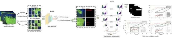
This section details the interference detection and segmentation experiments on the collected Sentinel-1 measured data to verify the efficiency of IQDN and the accuracy of SISNet. Furthermore, qualitative and quantitative metrics are involved in the evaluation of the performance of diverse intelligent algorithms on interference detection and segmentation. Real SAR images from the Sentinel-1 satellite are built as the MID and PAIS datasets and are used in the following experiments.

5.1. Results of the Interference Detection Experiment

Validating the time consumption and accuracy of the IQDN, we conduct experiments using test data of the MID Dataset mentioned in Section 3. The IQDN is trained on an NVIDIA GeForce RTX 3060 GPU. IQDN utilizes the Adam optimizer, and the batch size is set to 64. The learning rate is set to 0.01 and descends with a step-wise strategy. Figure 16a shows the growing tendency of training accuracy as more steps are taken by IQDN and some other CNNs. The IQDN accuracy gradually ascends to 100%. Figure 16b shows the loss curve with training steps. The loss drops rapidly as the model gradually converges. The curve demonstrates that the VGG model converges faster because pre-trained parameters are used during its training.
Then, we conduct a Monte Carlo experiment by selecting 100 images from the dataset that was not used in the training process and test them with trained model parameters. During this, the total time consumption is recorded. We divided the total time consumption by 100 to get the average inference time required to test a picture; the results are shown in Table 3 below:
We can draw a conclusion from the table that the IQDN network proposed in this paper can achieve faster inference speed than other CNNs. This means we can quickly screen out the data with RFI from massive SAR data and lay a solid foundation for subsequent work.
While detecting RFI efficiently, the proposed model also has a smaller number of parameters than VGG, ResNet, SENet, and MobileNet, as shown in Table 4, which theoretically proves that the IQDN is lighter than other CNNs.

5.2. Results of the Interference Segmentation Experiment

In this section, measured Sentinel-1 quick-look images of the PAIS dataset are used for validation and comparison. The RFI artifacts are annotated for ground truth. By conducting the aforementioned designs, the semantic segmentation capacity of SISNet is advanced. Then, the proposed SISNet is trained. To test the semantic segmentation performance of the proposed SISNet, we select some existing semantic segmentation networks such as FCN, Mask RCNN, UNet++, and U2Net, and train these networks with the same parameters; the results obtained are used as comparative test results. The training is carried out on an HP workstation in the school laboratory. The GPU used is a GeForce RTX 3060 12 GB, the CPU is an Intel i7-10700, and the computer has 64 GB of RAM. Due to the limitations of hardware conditions, the U2Net network parameters are too large, leaving us no other options but to run the U2NetP network, which is the lightweight version of U2Net, on the terminal. Therefore, the SISNet trained on the workstation is also formed based on U2NetP and the improvements mentioned above. Data augmentation automatically expands the training set by providing modified data from the original data. To estimate the quality of the segmentation, we use the five-fold cross-validation technique (i.e., training and validating five times) and present the averaged results. Thus, the dataset is randomly divided into a training subset and validation subset at a ratio of 4:1 in each training stage. To quantitatively prove the superiority of SISNet, we conduct hypothesis testing on the differences among indicators from test samples. All these experiments are performed in a similar pattern. For fair comparison, all state-of-the-art models are set with default, official, original parameters, such as the number of neurons and the number of network layers. In addition, the initial learning rate of training is 0.05 and descends in a polynomial form, and the model iterates for 50 epochs. During training, each epoch is iterated and becomes valid once, and the final result is the mIoU, accuracy, precision, and F1 score of the epoch when the mIoU is the highest.
The average mIoU of the proposed network and the networks used in the comparison test are calculated after the five-fold cross-validation training, as shown in Figure 17b below, and the change in the average loss is shown in Figure 17a. It can be concluded that the mIoU curve of SISNet fluctuates less, indicating the model can fit the training data well and has a stronger learning ability for unbalanced datasets. In addition, the mIoU curve of SISNet completely exceeds the mIoU curve of UNet and U2Net after the 30th epoch, showing that it can achieve better segmentation performance than U2Net. At last, the results show that after the 40th epoch, the error bars of SISNet’s mIoU and F1 curves do not overlap with those of other models, indicating that our method significantly improves segmentation performance.
In addition, when training SISNet, the five-fold cross-validation experiments are performed, and we present the mIoU results of five subtests with the average mIoU results in Figure 18a. The corresponding training loss of subtests and the average loss are show in Figure 18b. The combined average mIoU results of SISNet compared to different networks are added with the standard deviation in the form of vertical lines in individual epochs (see Figure 19). The common sense is that when the difference between the means of two samples is greater than two standard deviation, the change has significance. It can be further concluded from the figure that SISNet significantly improves RFI segmentation performance compared to other semantic segmentation networks.
After cross-validation experiments, the results of mIoU, accuracy, precision, and F1 of each network are shown in Table 5 following. The standard deviation is calculated from each subtest of the five-fold cross-validation method. In addition, the results of all indicators are selected based on the epoch with the best average score of mIoU.
The attained results in Table 5 point out that FCN exhibits poor performance for the RFI artifact segmentation task. The comparative validation results of UNet++ and UNet show that deepening the network does not necessarily improve the segmentation performance. At the same time, the experimental results of UNet and U2Net show that the lightweight U2Net can achieve similar performance under the premise of using fewer parameters, demonstrating the superiority of the U2Net network for the RFI artifact segmentation task. Finally, comparing the results of SISNet and U2Net, we can reach the conclusion that the improvements proposed in this paper can further improve the performance of U2Net.
To better demonstrate the good effect of SISNet on interference segmentation, we select six typical scenarios that were not used in training. These scenarios contain various land covers, such as mountains, lakes, seaside, and islands, as well as different types of RFI artifacts. The data acquisition orbit numbers of these scenarios are shown in Table 6.
During the experiment, we input the resized quick-look images of these scenarios into SISNet and other networks for comparative experiments. The output segmentation results obtained by each network are shown in Figure 20.
Through the comparison of the test results, we find that the segmentation mask output by SISNet is closest to the label image, and no matter how the size of the area occupied by the RFI artifact changes in the test image, the prediction mask output by the model has better performance in terms of mask integrity and numerical accuracy of RFI instances.
To illustrate the significant improvement the proposed model possesses over the comparison models, we conduct statistical analysis based on hypothesis testing on the tested indicator results. Because the samples in the test set are independent random samples, the sampling distribution conforms to the normal distribution as the sample size reaches 100, and indicators such as IoU are continuous variables, while the comparison between models is a categorical variable; it is suitable for hypothesis testing for two-sample cases. We conduct test experiments on 20 data samples randomly selected from the test set of the PAIS dataset and obtain the sample mean, sample standard deviation, etc. of the IoU and other indicators of the test set samples under different models. Take the IoU of SISNet and U2Net as an example. With small samples, the t distribution is used to establish the critical region. The formulas of the t distribution are expressed as follows:
t = μ 1 μ 2 σ μ 1 , μ 2 ,
σ μ 1 , μ 2 = N 1 σ 1 2 + N 2 σ 2 2 N 1 + N 2 2 N 1 + N 2 N 1 N 2 ,
where N 1 = N 2 = 20 , μ 1 stands for the sample mean of SISNet’s test IoU results, and the standard deviation is σ 1 . The sample mean of U2Net’s test IoU results is μ 2 , and the standard deviation is σ 2 . We set the confidence level at 95%, and the corresponding critical region is t ( c r i t i c a l ) = ± 2.002 in a two-tailed test. The null hypothesis H 0 can be established as μ 1 = μ 2 , and the alternative hypothesis H 1 is μ 1 μ 2 . If the obtained t score falls beyond the critical region, the null hypothesis is rejected, which means that H 1 is accepted and the mean of the IoU of the two groups is significantly different. The specific values of the sample mean and sample standard deviation of the IoU results of the above two tests are shown in Table 7 below. The t score obtained at this time is t ( o b t a i n e d ) = 4.361 .
Based on the statistics, it can be concluded that t ( o b t a i n e d ) falls out of the critical region, which means that the hypothesis H 0 is rejected. As a result, there exists a significant difference between the IoU sample means of the two groups of test results. Given the direction of the difference, we can also note that the average IoU result of SISNet outperforms U2Net’s.
Similarly, we can calculate the t score of each indicator of SISNet and compare it to other models one by one. The confidence level is set to 95%. By looking up to the t distribution table, we find that the critical region t ( c r i t i c a l ) = ± 2.002 . The calculated t scores are shown in Table 8 following, wherein the numbers with superscripts represent the significance of the test indicators of SISNet relative to the comparison models.
From the above results, since most t ( o b t a i n e d ) values fall outside of the critical region, it is obvious that the proposed SISNet significantly outperforms the other models in most indicators representing segmentation performance. Specifically, SISNet surpasses U2Net in IoU, accuracy and F1 score, while it is slightly inferior to U2Net in precision. Moreover, SISNet performs better than FCN8s, UNet, and UNet++ in all indicators, but the accuracy does not improve significantly in contrast to UNet++.
While achieving excellent segmentation performance, the proposed model has a smaller number of parameters and less computation than FCN, UNet, and UNet++, as shown in Table 9. Compared to the original U2Net, the SISNet proposed achieved a large improvement in image segmentation indicators such as mIoU and F1 score without significantly increasing the model parameters and computational load, which shows the superiority of SISNet.
It is worth mentioning that owing to the limited computing ability, the lightweight version of U2Net network is used in the experiment, but it still achieves better segmentation performance. If the improved technologies proposed in this article can be applied to the full version of U2Net, better results should be obtained in theory.
The ablation experiment exhibits the results of a neural network after removing essential modules to acknowledge the effect of these modules on the whole network. Therefore, we perform ablation experiments by discarding the RFB-d modules and attention modules. The experiments also conduct five-fold cross-validation in the training stage. Table 10 summarizes the average scores of mIoU, accuracy, precision, and F1 scores of diverse networks, which validates the usefulness of these modules.

6. Discussion

In this article, the IQDN based on modified MobileNetV2 and the SISNet are proposed. Compared to current algorithms, the IQDN employs a lightweight CNN to capture the characteristic differences between images with RFI artifacts and without RFI artifacts. MobileNet has a strong feature extraction ability and few network parameters. Therefore, it performs well in both speed and accuracy for detecting whether there is interference in quick-look images, which is beneficial for building an automatic interference identification system that searches and screens RFI artifacts in massive SAR data.
Methods proposed by previous researchers are either poor in robustness or require a large amount of non-interference comparison SAR data, which restricts their application. This paper introduces an interference segmentation algorithm called SISNet. Different from previous work, the SISNet performs well in interference segmentation and does not require interference-free comparison data, which reduces the difficulty of implementation. After performing image transformation on the segmentation mask image output from the network according to the latitude and longitude information and image size information of the SLC or GRD products, the output image can be connected to Google Earth Engine [57] to be combined with actual geographic information in order to realize SAR interference positioning. However, it is worth mentioning that the training data of SISNet still needs to be manually labeled, and the impact of the interference multi-scale problem has not been completely solved, which means further improvements are still needed. Future research will add more interference-affected data to facilitate the functionality of our framework.

7. Conclusions

In this article, we first build two new datasets, named the ’MID dataset’ and the ’PAIS dataset’, using Sentinel-1 SAR quick-look images for RFI detection and segmentation tasks. Then, we present IQDN on the basis of MobileNet, which provides a novel RFI detector to quickly and precisely detect RFI in the image domain of the MID dataset. The test experiment shows IQDN is less time-consuming than other CNNs. In addition, we propose an RFI segmentation network named SISNet based on U2Net. It distinguishes RFI artifacts from terrain and ocean background by automatically outputting a pixel-level predicted mask, which can be used in RFI localization by combining the corresponding product information. Moreover, four different metrics, including mIoU, accuracy, precision, and F1 score, are adopted to assess the performance of SISNet. Statistical analysis based on the validation results and hypothesis testing indicate that SISNet outperforms state-of-the-art methods in RFI segmentation performance on the PAIS dataset. It not only saves researchers from searching for a large amount of interference-free contrast data but also realizes the preliminary localization of RFI through image segmentation.

Author Contributions

J.Z. designed the experiment; J.Z. and Y.Z. analyzed the data; J.Z., X.L., X.Z. and C.Y. performed the experiments; J.Z. wrote the paper; X.Z., G.L. and Y.W. supervised the program; X.Z. revised the grammar errors of the paper; H.X. improved the English writing; K.L., C.Y., Y.Z. and X.L. were responsible for data collection, classification, and labeling. All authors have agreed to publish the current version of the manuscript.

Funding

This paper was funded partially by the Youth Project of High-Level Talent Recruiting Plan of Shaanxi Province (90728220019) and was co-financed by the Science and Technology Innovation Team of Shaanxi Province (2022TD-38).

Data Availability Statement

The data that support the findings of this study are openly available on the official website of European Space Agency at https://scihub.copernicus.eu/dhus/#/home, accessed on 9 September 2023).

Acknowledgments

The authors appreciate all the anonymous reviewers and editors for their constructive comments and suggestions that greatly improved this paper. Meanwhile, the authors are thankful to the European Space Agency for providing free online downloading of the Sentinel-1 data.

Conflicts of Interest

The authors declare no conflict of interest.

Abbreviations

The following abbreviations are used in this manuscript:
SARSynthetic Aperture Radar
CNNConvolutional Neural Network
DCNNDeep Convolutional Neural Network
RFIRadio Frequency Interference
SISNetSmart Interference Segmentation Network
RELURectified Linear Units
IQDNInterference-targeted Quick Detection Network
IoUIntersection over Union
RFBReceptive Field Block
RFReceptive Field
SLCSingle Look Complex
GRDGround Range Detected
IWInterferometric Wide
RSUResidual U Block
CBAMConvolutional Block Attention Module
LCBAMLightweight Convolutional Block Attention Module
ASPPAtrous Spatial Pyramid Pooling
MIDMulti-scale Interference Detection
PAISPolygonal-annotated Interference Segmentation
MLPMulti-layer Perceptron
RGBRed–Green–Blue
SSDSingle-Shot Multi-Box Detector

References

  1. Tao, M.; Su, J.; Huang, Y.; Wang, L. Mitigation of Radio Frequency Interference in Synthetic Aperture Radar Data: Current Status and Future Trends. Remote Sens. 2019, 11, 2438. [Google Scholar] [CrossRef]
  2. Ding, X.L.; Li, Z.W.; Zhu, J.J.; Feng, G.C.; Long, J.P. Atmospheric Effects on InSAR Measurements and Their Mitigation. Sensors 2008, 8, 5426–5448. [Google Scholar] [CrossRef] [PubMed]
  3. Yang, L.; Zheng, H.; Feng, J.; Li, N.; Chen, J. Detection and suppression of narrow band RFI for synthetic aperture radar imaging. Chin. J. Aeronaut. 2015, 28, 1189–1198. [Google Scholar] [CrossRef]
  4. Yu, J.; Li, J.; Sun, B.; Chen, J.; Li, C. Multiclass Radio Frequency Interference Detection and Suppression for SAR Based on the Single Shot MultiBox Detector. Sensors 2018, 18, 4034. [Google Scholar] [CrossRef] [PubMed]
  5. Wang, J.; Yu, W.; Deng, Y.; Wang, R.; Wang, Y.; Zhang, H.; Zheng, M.T. Demonstration of Time-Series InSAR Processing in Beijing Using a Small Stack of Gaofen-3 Differential Interferograms. J. Sens. 2019, 2019, 4204580. [Google Scholar] [CrossRef]
  6. Zebker, H.A.; Rosen, P.A.; Hensley, S. Atmospheric effects in interferometric synthetic aperture radar surface deformation and topographic maps. J. Geophys. Res. 1997, 102, 7547–7563. [Google Scholar] [CrossRef]
  7. Emardson, T.R.; Simons, M.; Webb, F.H. Neutral atmospheric delay in interferometric synthetic aperture radar applications: Statistical description and mitigation. J. Geophys. Res. 2003, 108, 2231–2238. [Google Scholar] [CrossRef]
  8. Nie, G.L.; Liao, G.S.; Zeng, C.; Zhang, X.P.; Li, D.C. Joint Radio Frequency Interference and Deceptive Jamming Suppression Method for Single-Channel SAR via Subpulse Coding. IEEE J. Sel. Top. Appl. Earth Obs. Remote Sens. 2022, 16, 787–798. [Google Scholar] [CrossRef]
  9. Tao, M.L.; Li, J.S.; Chen, J.L.; Liu, Y.Y.; Fan, Y.F.; Su, J.; Wang, L. Radio frequency interference signature detection in radar remote sensing image using semantic cognition enhancement network. IEEE Trans. Geosci. Remote Sens. 2022, 60, 1–14. [Google Scholar] [CrossRef]
  10. Meyer, F.J.; Nicoll, J.B.; Doulgeris, A.P. Correction and Characterization of Radio Frequency Interference Signatures in L-Band Synthetic Aperture Radar Data. IEEE Trans. Geosci. Remote Sens. 2013, 51, 4961–4972. [Google Scholar] [CrossRef]
  11. Njoku, E.; Ashcroft, P.; Chan, T.; Li, L. Global survey and statistics of radio-frequency interference in AMSR-E land observation. Geosci. Remote Sens. 2005, 43, 938–947. [Google Scholar] [CrossRef]
  12. Ellingson, S.W.; Johnson, J.T. A polarimetric Survey of Radio Frequency Interference in C and X bands in the Continental United States using WindSat Radiometry. IEEE Trans. Geosci. Remote Sens. 2006, 44, 540–548. [Google Scholar] [CrossRef]
  13. Draped, D.W.; de Matthaeis, P.P. Characteristics of 18.7 GHZ Reflected Radio Frequency Interference in Passive Radiometer Data. In Proceedings of the IGARSS 2019—2019 IEEE International Geoscience and Remote Sensing Symposium, Yokohama, Japan, 28 July–2 August 2019; pp. 4459–4462. [Google Scholar]
  14. Antoni, J. The spectral kurtosis: A useful tool for characterizing non-stationary signals. Mech. Syst. Signal Process. 2006, 20, 282–307. [Google Scholar] [CrossRef]
  15. De Roo, R.D.; Misra, S.; Ruf, C.S. Sensitivity of the Kurtosis statistic as a detector of pulsed sinusoidal RFI. IEEE Trans. Geosci. Remote Sens. 2007, 45, 1938–1946. [Google Scholar] [CrossRef]
  16. Jarque, C.M.; Bera, A.K. A Test for normality of observations and regression residuals. Intern. Statist. Rev. 1987, 55, 163–172. [Google Scholar] [CrossRef]
  17. Parasher, P.; Aggarwal, K.M.; Ramanujam, V.M. RFI detection and mitigation in SAR data. In Proceedings of the Conference: 2019 URSI Asia-Pacific Radio Science Conference (AP-RASC), New Delhi, India, 9–15 March 2019. [Google Scholar]
  18. Monti-Guarnieri, A.; Giudici, D.; Recchia, A. Identification of C-Band Radio Frequency Interferences from Sentinel-1 Data. Remote Sens. 2017, 9, 1183. [Google Scholar] [CrossRef]
  19. Tao, M.; Lai, S.; Li, J.; Su, J.; Fan, Y.; Wang, L. Extraction and mitigation of radio frequency interference artifacts based on time-series Sentinel-1 SAR data. IEEE Trans. Geosci. Remote Sens. 2021, 60, 1–11. [Google Scholar] [CrossRef]
  20. Li, N.; Zhang, H.; Lv, Z.; Min, L.; Guo, Z. Simultaneous Screening and Detection of RFI From Massive SAR Images: A Case Study on European Sentinel-1. IEEE Trans. Geosci. Remote Sens. 2022, 60, 1–17. [Google Scholar] [CrossRef]
  21. Leng, X.; Ji, K.; Kuang, G. Radio frequency interference detection and localization in Sentinel-1 images. IEEE Trans. Geosci. Remote Sens. 2021, 59, 9270–9281. [Google Scholar] [CrossRef]
  22. Zhang, L.; You, W.; Wu, Q.M.J.; Qi, S.; Ji, Y. Deep Learning-Based Automatic Clutter/Interference Detection for HFSWR. Remote Sens. 2018, 10, 1517. [Google Scholar] [CrossRef]
  23. Akeret, J.; Chang, C.; Lucchi, A.; Refregier, A.A. Radio frequency interference mitigation using deep convolutional neural networks. Astron. Comput. 2017, 18, 35–39. [Google Scholar] [CrossRef]
  24. Fan, W.; Zhou, F.; Tao, M.; Bai, X.; Rong, P.; Yang, S.; Tian, T. Interference Mitigation for Synthetic Aperture Radar Based on Deep Residual Network. Remote Sens. 2019, 11, 1654. [Google Scholar] [CrossRef]
  25. Sandler, M.; Andrew, H.; Zhu, M.L.; Andrey, Z.; Chen, L.C. Mobilenetv2: Inverted residuals and linear bottlenecks. In Proceedings of the IEEE Conference on Computer Vision and Pattern Recognition, Salt Lake City, UT, USA, 18–23 June 2018; pp. 4510–4520. [Google Scholar]
  26. Huang, Y.; Zhao, B.; Tao, M.L.; Chen, Z.Y.; Hong, W. Review of synthetic aperture radar interference suppression. J. Radars 2020, 9, 86–106. [Google Scholar]
  27. Ali, I.; Cao, S.; Naeimi, V.; Paulik, C.; Wagner, W. Methods to Remove the Border Noise From Sentinel-1 Synthetic Aperture Radar Data: Implications and Importance For Time-Series Analysis. IEEE J. Sel. Top. Appl. Earth Obs. Remote Sens. 2018, 11, 777–786. [Google Scholar] [CrossRef]
  28. ESA. Sentinel Online Technical Website. Sentinel-1. 2020. Available online: https://sentinel.esa.int/web/sentinel/missions/sentinel-1 (accessed on 23 July 2020).
  29. Copernicus Open Access Hub. 2014. Available online: https://scihub.copernicus.eu/dhus/#/home (accessed on 28 October 2014).
  30. Krizhevsky, A.; Sutskever, I.; Hinton, G. ImageNet classification with deep convolutional neural networks. In Proceedings of the 2012 Advances in Neural Information Processing Systems (NIPS), Lake Tahoe, NV, USA, 3–6 December 2012; pp. 1097–1105. [Google Scholar]
  31. Simonyan, K.; Zisserman, A. Very deep convolutional networks for large-scale image recognition. In Proceedings of the 2015 International Conference Learning Representations (ICLR), New York, NY, USA, 7–9 May 2015; pp. 1–14. [Google Scholar]
  32. He, K.; Zhang, X.; Ren, S.; Sun, J. Deep residual learning for image recognition. In Proceedings of the 2016 IEEE Conference on Computer Vision and Pattern Recognition (CVPR), Las Vegas, NV, USA, 26 June–1 July 2016; pp. 770–778. [Google Scholar]
  33. Girshick, R.; Donahue, J.; Darrell, T.; Malik, J. Rich feature hierarchies for accurate object detection and semantic segmentation. In Proceedings of the 2014 IEEE Conference on Computer Vision and Pattern Recognition (CVPR), Columbus, OH, USA, 23–28 June 2014; pp. 580–587. [Google Scholar]
  34. Ren, S.; He, K.; Girshick, R.; Sun, J. Faster r-cnn: Towards real-time object detection with region proposal networks. IEEE Trans. Pattern Anal. Mach. Intell. 2017, 39, 1137–1149. [Google Scholar] [CrossRef] [PubMed]
  35. Redmon, J.; Divvala, S.; Girshick, S.; Farhadi, A. You only look once: Unified, real-time object detection. In Proceedings of the 2016 IEEE Computer Society Conference on Computer Vision and Pattern Recognition (CVPR), Las Vegas, NV, USA, 26 June–1 July 2016; pp. 779–788. [Google Scholar]
  36. Shelhamer, E.; Long, J.; Darrell, T. Fully convolutional networks for semantic segmentation. IEEE Trans. Pattern Anal. Mach. Intell. 2017, 39, 640–651. [Google Scholar] [CrossRef] [PubMed]
  37. Dronner, J.; Korfhage, N.; Egli, S.; Muhling, M.; Thies, B.; Bendix, J.; Freisleben, B.; Seeger, B. Fast cloud segmentation using convolutional neural networks. Remote Sens. 2018, 10, 1782. [Google Scholar] [CrossRef]
  38. Noh, H.; Hong, S.; Han, B. Learning deconvolution network for semantic segmentation. In Proceedings of the 2015 IEEE International Conference on Computer Vision (ICCV), Santiago, Chile, 11–18 December 2015; pp. 1520–1528. [Google Scholar]
  39. Howard, A.G.; Zhu, M.; Chen, B.; Kalenichenko, D.; Wang, W.; Weyand, T.; Andreetto, M.; Adam, H. Mobilenets: Efficient Convolutional Neural Networks for Mobile Vision Applications. Available online: https://arxiv.org/abs/1704.04861 (accessed on 17 April 2017).
  40. Lei, T.; Asoke, K.N. Image Segmentation: Principles, Techniques, and Applications; John Wiley & Sons: Hoboken, NJ, USA, 2022. [Google Scholar]
  41. Tokarczyk, P.; Jan Dirk, W.; Stefan, W.; Konrad, S. Features, color spaces, and boosting: New insights on semantic classification of remote sensing images. IEEE Trans. Geosci. Remote Sens. 2014, 53, 280–295. [Google Scholar] [CrossRef]
  42. Dakhia, A.; Tiantian, W.; Huchuan, L. Multi-scale pyramid pooling network for salient object detection. Neurocomputing 2019, 333, 211–220. [Google Scholar] [CrossRef]
  43. Jonathan, L.; Evan, S.; Trevor, D. Fully Convolutional Networks for Semantic Segmentation. In Proceedings of the IEEE Conference on Computer Vision and Pattern Recognition (CVPR), Boston, MA, USA, 7–12 June 2015; pp. 3431–3440. [Google Scholar]
  44. Krizhevsky, A.; Ilya, S.; Geoffrey, E.H. Imagenet classification with deep convolutional neural networks. Adv. Neural Inf. Process. Syst. 2012, 25, 84–90. [Google Scholar] [CrossRef]
  45. Ronneberger, O.; Fischer, P.; Brox, T. U-net: Convolutional networks for biomedical image segmentation. In Proceedings of the Medical Image Computing and Computer-Assisted Intervention–MICCAI 2015: 18th International Conference, Munich, Germany, 5–9 October 2015; Part III 18. pp. 234–241. [Google Scholar]
  46. Alom, M.Z.; Yakopcic, C.; Hasan, M.; Taha, T.M.; Asari, V.K. Recurrent residual U-Net for medical image segmentation. J. Med. Imaging 2019, 6, 014006. [Google Scholar] [CrossRef]
  47. Oktay, O.; Schlemper, J.; Folgoc, L.L.; Lee, M.; Heinrich, M.; Misawa, K.; Mori, K.; McDonagh, S.; Hammerla, N.Y.; Kainz, B.; et al. Attention u-Net: Learning Where to Look for the Pancreas. Available online: https://arxiv.org/abs/1804.03999 (accessed on 11 April 2018).
  48. Zhou, Z.; Rahman Siddiquee, M.M.; Nima, T.; Liang, J. Unet++: A nested u-net architecture for medical image segmentation. In Proceedings of the Deep Learning in Medical Image Analysis and Multimodal Learning for Clinical Decision Support: 4th International Workshop, DLMIA 2018, and 8th International Workshop, ML-CDS 2018, Held in Conjunction with MICCAI 2018, Granada, Spain, 20 September 2018; Volume 4, pp. 3–11. [Google Scholar]
  49. Qin, X.; Zhang, Z.; Huang, C.; Dehghan, M.; Zaiane, O.R.; Jagersand, M. U2-Net: Going deeper with nested U-structure for salient object detection. Pattern Recogn 2020, 106, 107404. [Google Scholar] [CrossRef]
  50. Chen, L.C.; George, P.; Iasonas, K.; Kevin, M.; Alan, L.Y. Semantic Image Segmentation with Deep Convolutional Nets and Fully Connected Crfs. Available online: https://arxiv.org/abs/1412.7062 (accessed on 22 December 2014).
  51. Woo, S.; Park, J.; Lee, J.-W.; Kweon, I.S. Cbam: Convolutional block attention module. In Proceedings of the European Conference on Computer Vision (ECCV), Munich, Germany, 8–14 September 2018; pp. 3–19. [Google Scholar]
  52. Han, K.; Wang, Y.; Tian, Q.; Guo, J.; Xu, C.; Xu, C. Ghostnet: More features from cheap operations. In Proceedings of the IEEE/CVF Conference on Computer Vision and Pattern Recognition, Seattle, WA, USA, 13–19 June 2020; pp. 1580–1589. [Google Scholar]
  53. Stevens, E.; Luca, A.; Thomas, V. Deep Learning with PyTorch; Manning Publications: Shelter Island, NY, USA, 2020. [Google Scholar]
  54. Zhang, R. Making convolutional networks shift-invariant again. In Proceedings of the 36th International Conference on Machine Learning, Long Beach, CA, USA, 9–15 June 2019; pp. 7324–7334. [Google Scholar]
  55. Lin, T.Y.; Priya, G.; Ross, G.; Kaiming, H.; Piotr, D. Focal loss for dense object detection. In Proceedings of the IEEE International Conference on Computer Vision, Venice, Italy, 22–29 October 2017; pp. 2980–2988. [Google Scholar]
  56. Liu, S.; Di, H. Receptive field block net for accurate and fast object detection. In Proceedings of the European Conference on Computer Vision (ECCV), Munich, Germany, 8–14 September 2018; pp. 385–400. [Google Scholar]
  57. Zhao, Q.; Yu, L.; Li, X.; Peng, D.; Zhang, Y.; Gong, P. Progress and trends in the application of Google Earth and Google Earth Engine. Remote Sens. 2021, 13, 3778. [Google Scholar] [CrossRef]
Figure 1. RFI-contaminated Sentinel-1 data examples.
Remotesensing 15 05462 g001
Figure 2. A rough classification of SAR interference [26].
Remotesensing 15 05462 g002
Figure 3. Some samples of the MID dataset. (left) RFI-contaminated images. (right) RFI-free images.
Remotesensing 15 05462 g003
Figure 4. The data augmentations performed, including flipping, blurring, translating, and affiliating.
Remotesensing 15 05462 g004
Figure 5. Some augmented data samples of PAIS dataset show from left to right in columns that the original image has been flipped, translated and blurred, and noise has been added, respectively.
Remotesensing 15 05462 g005
Figure 6. Samples of PAIS dataset. (a,c,e,g) are quick-look images contaminated by RFI. (b,d,f,h) are the annotated segmentation labels.
Remotesensing 15 05462 g006
Figure 7. Schematic diagram of FCN network.
Remotesensing 15 05462 g007
Figure 8. Schematic diagram of UNet.
Remotesensing 15 05462 g008
Figure 9. Architecture of proposed IQDN.
Remotesensing 15 05462 g009
Figure 10. Ghost module: replacing convolution operation with linear transformation.
Remotesensing 15 05462 g010
Figure 11. Max-Blur-Pooling: an anti-aliasing max-pooling method implemented by applying low-pass filters before down-sampling.
Remotesensing 15 05462 g011
Figure 12. The architecture of the modified receptive field block with larger dilation rates.
Remotesensing 15 05462 g012
Figure 13. The framework of the channel weighting module.
Remotesensing 15 05462 g013
Figure 14. Modified convolutional layer with shortcut layer between input and output.
Remotesensing 15 05462 g014
Figure 15. The network structure of proposed SISNet.
Remotesensing 15 05462 g015
Figure 16. The training accuracy and loss curve with training steps: (a) training accuracy; (b) loss.
Remotesensing 15 05462 g016
Figure 17. The average training loss curve and evaluation indicators of different networks with training epochs. Error bars were added in the last 10 epochs: (a) average training loss, (b) average training mIoU, (c) average training precision, and (d) average training F1.
Remotesensing 15 05462 g017
Figure 18. The SISNet training mIoU curve and loss curve with training epochs in the five-fold cross-validation experiments: (a) the mIoU results of five subtests and the average mIoU and (b) the loss of five subtests and the average loss.
Remotesensing 15 05462 g018
Figure 19. Comparison of average mIoU results of different semantic segmentation networks. Validation method: 5-fold cross-validation. (a) SISNet vs. FCN8s, (b) SISNet vs. UNet, (c) SISNet vs. UNet++, and (d) SISNet vs. U2Net.
Remotesensing 15 05462 g019
Figure 20. Comparison of interference segmentation experiment results: (a1a6) original quick-look images (the numbering sequence is consistent with Table 5 above); (b1b6) label image; (c1c6) FCN8s outputs; (d1d6) UNet++ outputs; (e1e6) U2Net outputs; (f1f6) our proposed SISNet outputs.
Remotesensing 15 05462 g020
Table 1. General information of MID dataset.
NameObservation AreaTime SpanInterference
Sample Quantity
Interference-Free
Sample Quantity
Image Size
MID datasetKorea1 May 2021–30 May 202225,66522,270224 × 224
Table 2. General information of PAIS dataset.
NameObservation AreaTime SpanTrain Sample
Quantity
Test Sample
Quantity
Image Size
PAIS datasetKorea1 May 2021–30 May 20222000100572 × 572
Table 3. Comparison of the mean inference time per image of different models.
ModelVGGResNet50SENetMobileNetV2Ours
time (ms)8.017.029.046.996.10
Table 4. Comparison of model size of different interference detection networks used in experiments.
ModelVGGResNet50SENetMobileNetV2Ours
Parameters (M)138.3523.5126.022.221.68
Flops (G)15.484.094.105.555.51
Table 5. Comparison of 5-fold cross-validation results with ± one standard deviation value of different semantic segmentation networks on PAIS dataset.
ModelMask RCNNFCN8sUNetUNet++U2Net 1Ours
mIoU (%)77.05 ± 0.3872.69 ± 0.1285.68 ± 0.1279.33±0.4085.38 ± 0.2187.46 ± 0.26
Accuracy (%)/95.16 ± 0.2097.63 ± 0.0696.56 ± 0.0397.61 ± 0.0598.01 ± 0.06
Precision (%)77.55 ± 0.1874.16 ± 1.9387.70 ± 1.0483.72 ± 0.1887.76 ± 0.2889.15 ± 0.48
F1 (%)75.46 ± 1.5266.68 ± 0.7484.97 ± 0.0576.89 ± 0.6284.74 ± 0.2287.09 ± 0.76
1 Here refers to the U2NetP network.
Table 6. The data acquisition orbit numbers of the scenarios used in the RFI segmentation experiment.
Scene NumberData Acquisition Orbit Number
1S1A_IW_GRDH_1SDV_20210629T155008_20210629T155033_038557_048CBF_FE4A
2S1A_IW_GRDH_1SDV_20210815T150830_20210815T150855_039242_04A202_A30A
3S1B_IW_GRDH_1SDV_20210701T034259_20210701T034324_027595_034B3C_0452
4S1B_IW_GRDH_1SDV_20210805T154051_20210805T154116_028113_035A96_4115
5S1A_IW_SLC_1SDV_20220124T031552_20220124T031619_041597_04F2A1_B042
6S1B_IW_GRDH_1SDV_20210607T094904_20210607T094932_027249_03413A_E4CB
Table 7. Sample means and sample standard deviation of SISNet’s and U2Net’s test IoU results.
ModelSISNetU2Net 1
Sample mean ( μ ) μ 1 = 91.05 μ 2 = 88.15
Sample standard deviation ( σ ) σ 1 = 2.39 σ 2 = 1.64
1 Here refers to the U2NetP network.
Table 8. The t scores of evaluation indicators of SISNet compared to other models.
ModelFCN8sUNetUNet++U2Net 1
t(obtained) of IoU9.299 **3.910 **3.356 **4.361 **
t(obtained) of Accuracy3.222 **3.631 **0.0846.236 **
t(obtained) of Precision7.604 **2.651 *3.223 **−1.178
t(obtained) of F18.670 **5.477 **3.084 **4.277 **
1 Here refers to the U2NetP network. Note: n = 20, * p < 0.05, ** p < 0.01.
Table 9. Comparison of model size of different semantic segmentation networks used in experiments.
ModelFCN8sUNetUNet++U2Net 1Ours
Parameters (M)33.6034.5336.631.271.27
Flops (G)104.81262.10554.6571.4776.56
1 Here refers to the U2NetP network.
Table 10. Results of ablation experiments.
Ablation ApproachesmIoUAccuracyPrecisionF1
No improvements (%)85.3897.6187.7684.74
No RFB-d (%)87.0397.9088.0186.55
No attention modules (%)86.5497.8187.9986.02
Proposed (%)87.4698.0189.1587.09
Disclaimer/Publisher’s Note: The statements, opinions and data contained in all publications are solely those of the individual author(s) and contributor(s) and not of MDPI and/or the editor(s). MDPI and/or the editor(s) disclaim responsibility for any injury to people or property resulting from any ideas, methods, instructions or products referred to in the content.

