OEGR-DETR: A Novel Detection Transformer Based on Orientation Enhancement and Group Relations for SAR Object Detection

Abstract

Object detection in SAR images has always been a topic of great interest in the field of deep learning. Early works commonly focus on improving performance on convolutional neural network frameworks. More recent works continue this path and introduce the attention mechanisms of Transformers for better semantic interpretation. However, these methods fail to treat the Transformer itself as a detection framework and, therefore, lack the development of various details that contribute to the state-of-the-art performance of Transformers. In this work, we first base our work on a fully multi-scale Transformer-based detection framework, DETR (DEtection TRansformer) to utilize its superior detection performance. Secondly, to acquire rotation-related attributes for better representation of SAR objects, an Orientation Enhancement Module (OEM) is proposed to facilitate the enhancement of rotation characteristics. Then, to enable learning of more effective and discriminative representations of foreground objects and background noises, a contrastive-loss-based GRC Loss is proposed to preserve patterns of both categories. Moreover, to not restrict comparisons exclusively to maritime objects, we have also developed an open-source labeled vehicle dataset. Finally, we evaluate both detection performance and generalization ability on two well-known ship datasets and our vehicle dataset. We demonstrated our method’s superior performance and generalization ability on both datasets.

1. Introduction

Object detection in synthetic-aperture radar (SAR) images has always been of great research interest as deep learning methods become more accurate and intelligent. SAR images are obtained by microwave payloads and have distinct visual attributes that enable detection in various climate conditions, but at a cost, requiring more specialized treatment of input images. Under these premises, common detection approaches [1,2,3,4,5,6,7,8,9,10,11] focus on developing feature extraction, enhancement and de-noising modules as framework extensions, aiming to enable more specialized representations of SAR objects and minimize interference of speckle noises that are usually confused with foreground targets. Among these works, convolutional attention mechanisms [5,7] are some of the most effective mechanisms implemented and open up designs of more complex feature enhancement modules that utilize attention mechanisms. More recent works [12,13,14,15,16,17,18,19,20,21,22,23] have integrated components of Transformers into CNN detection frameworks and proved the capability of non-convolutional attention mechanisms in SAR object detection tasks.

The non-convolutional attention mechanisms were first introduced in the research of Transformers [24], which are a fully attention-based architecture originally designed for Natural Language Processing (NLP) tasks. Transformers use attention to extract global dependencies while suppressing irrelevant connections. This core concept is first utilized in vision tasks by the Vision Transformer (ViT) [25], and then its potential in object detection in Natural Images (NI) was then found shortly after by the DETR (DEtection TRansformer) [26], and its following developed models [27,28,29,30,31,32,33] gradually became the state-of-the-art methods in NI object detection.

Thanks to these recent developments, Transformer models have also exhibited promising performance in the detection of optical remote-sensing images (RSI). Among them, some studies focus on continuing to use Transformers as the backbone network and seek to improve internal mechanisms of attention variants [34]. Other studies follow the original designs of Transformers and overcome conflicts in direct knowledge transfer with their proposed extensions [35,36]. Works that directly implement Transformers as detection frameworks also achieved desirable results in their detection tasks [37,38,39,40,41,42]. Although these developments of Transformer detection models in optical RSI look promising, these Transformer-based methods have then turned their focus on improving the feature representation ability of Transformer networks or continuing the paths to implement more specialized improvements related to optical images. Meanwhile, SAR images, similar to optical RSI, also have significant scale variations, irregular distribution patterns of objects, and complex backgrounds. These attributes are mostly handled by multi-scale pyramid networks in previous studies, and pyramid networks continue to be effective in the aforementioned Transformer-based studies. But on top of these shared attributes, several vital differences between optical RSI and SAR images are not fully taken into consideration by optical methods, as we have shown below, and are still left to be properly handled with specialized designs.

As is shown in Figure 1a, objects in SAR images no longer have the rotation-invariant property that is common for optical objects. The characteristics of optical objects remain consistent with their rotated versions, as is shown in Figure 2a. However, due to the SAR imaging mechanism, the same object photoed at different orientation conditions often contains significant variations in their visual attributes, especially in the more complex detection scenarios shown in Figure 2b, therefore making rotation a crucial factor in learning feature representations. Moreover, the classification of objects in SAR images is overly generalized, which is not common for optical images which have multiple categories for different instances. As is shown in Figure 1b, for objects even of the same orientation status, details can still vary significantly. Not only does the foreground class have considerable intra-class variations, but noises that belong to the background class can also have noticeable variations and complicated patterns that can be confused with foreground objects. This property also requires improvements in enriching class information for SAR objects.

In this article, we develop our method following the content de-noising mechanism (CDN) applied in later DETR works [30,31]. The CDN mechanism enables more robust representation learning and has been proven to contribute to faster convergence speed of DETR models. To tackle the aforementioned challenges, we propose an Orientation Enhancement Module (OEM) to integrate Rotation-Sensitive features into the extracted feature sequence, and Grouped Relation Contrastive Loss (GRC Loss) integrated into the CDN mechanism to handle the intra-class variation problem of the over-generalized foreground and background classes. Extensive experiments on HRSID [43] and SSDD [44] are performed to validate the effectiveness and generalization ability of our method. Finally, to validate the robustness of our method in more challenging environments, we developed an SAR Vehicle Dataset and conducted experiments on this dataset. The main contributions of this article can be summarized as follows.

• We propose a novel object detector named OEGR-DETR for SAR images, which is the first detector in this task to implement the Transformer itself as the detection framework with specialized improvements regarding the rotation-variant properties and variations within and between classes, which are both vital characteristics of SAR objects.
• Considering rotation as a crucial factor for SAR object representation, we designed the Orientation Enhancement Module (OEM) to apply additional Rotation-Sensitive information into the feature sequence, which is absent in the original design.
• We designed the Grouped Relation Contrastive Loss (GRC Loss) to enable the learning of more discriminative representations of binary class features, with additional patterns to back up intra-class variations in SAR images.
• We conducted extensive experiments on the HRSID and SSDD datasets and achieved state-of-the-art performance on both datasets. We also found our method the most competitive for the generalization ability in the migration experiment.
• We developed a labeled dataset for vehicles in SAR images, conducted extensive comparisons with related methods, and have also achieved optimal performance.

We organize the remainder of this article as follows. We describe related works in Section 2 and introduce our proposed method in Section 3. In Section 4, we present the evaluations on two public datasets and evaluation on our SAR Vehicle Dataset. Then, we discuss the functions and effects of our proposed improvements in Section 5 and finally, we draw our conclusions in Section 6.

2. Related Works

2.1. Current Mainstream CNN-Based SAR Object Detection Methods

Current mainstream CNN detection methods in SAR images mainly focus on improving various feature extraction bottlenecks within CNN frameworks. But implementations of CNN-based attention in various methods have shown promising effects and therefore attracted interest. For one-stage networks, Du et al. [2] developed a saliency-based method on the SSD framework [45]. Ma et al. [3] proposed a convolution-based channel attention module in their YOLO-like architecture [46] to highlight object features. Cui et al. [4] developed a Shuffle-Group Enhance Attention module with group convolution on the CenterNet framework to capture local and global correlations while suppressing background noise. Hu et al. [6] designed their frameworks following RetinaNet architecture. They propose a Local Attention Module (LAM) with Deformable Convolution for local feature extraction. They also proposed the Non-local Attention Module (NLAM) with Depth-wise Convolution to perform pixel-wise attention re-weighting. Zhu et al. [7] based their convolution-based attention on RetinaNet architecture. They proposed an information compensation module (ICM) to extract and aggregate diverse spatial contextual information, as well as a feature enhancement module (FEM) to integrate object features from multiple levels. For two-stage networks, Kang et al. [8] and Li et al. [9] derived their methods from the Faster R-CNN framework for object detection in SAR images. Then, Lin et al. [10] leveraged Squeeze-and-Excitation (SE) [47], a CNN-based attention on the Faster R-CNN framework and achieved improved performance. Zhao et al. [11] developed their convolution-based mechanism over CBAM [48] in the Faster R-CNN framework.

2.2. Detr for Object Detection in Remote-Sensing Images

Transformers have long expressed high performance across fields of Natural Language Processing and computer vision, while in the latter, as for object detection in natural images, Transformer-based DETR frameworks are currently state-of-the-art detection models. The high performance continued to exist in remote-sensing images. Ma, Mao, et al. [37] first introduced DETR into oriented optical object detection. Dai et al. [38] then validated on optical RSIs the compatibility of Deformable DETR, and successfully leveraged multi-scale feature maps that are essential to all detection methods but too costly for dense-sampling DETR methods. They also proposed oriented proposal generation (OPG) and feature refinement modules (FRMs) to better adapt to features of oriented objects. Lee, Hakjin, et al. [42] then continued the development of DETR architecture and focused on dealing with innate problems of the Hungarian matching strategy. Zeng et al. [39] approached optical detection from the orientation perspective and developed rotation-related classification, de-noising, and feature re-weighting modules. Wang et al. [34] derived their Rotated VSA module, named RVSA, also reducing the computational cost of self-attention with the help of size-varied window-based attention. Sun et al. [35] proposed to utilize Masked Image Modeling (MIM) [49], which is a common training strategy for Transformer-based models, and contrastive loss [50] to learn task-related representations from optical RSIs in a self-supervised fashion. These methods focus on various challenges in optical detection and form their solutions based on observations and previous studies on optical images. Nevertheless, these improvements base their conclusions on the premise that diversity of objects exists in well-divided categories and background can often be easily distinguished from foreground objects. In SAR images, these prerequisites do not exist and hence need to be handled by specialized designs.

2.3. Transformers for SAR Object Detection

Convolutional attention mechanisms have revealed their potential in SAR object detection. In more recent research, the detection performance of non-convolutional attention mechanisms has been proven in optical images, leading to a shift of research focus in SAR object detection. In the realm of SAR object detection, the Transformer method diverges significantly from CNN networks. Transformer stands not merely as a substitute for CNN networks but also as a pivotal methodology, occasionally serving as the sole approach, for introducing cross-modality and establishing expansive foundational models. It has also presented an additional avenue for incorporating various modalities, such as textual data, into SAR object detection. Consequently, the advancements achieved by Transformer-based detectors are crucial, as they pave the way for potential research endeavors aiming to integrate multiple modalities into fundamental detectors. This, in turn, could lead to broader and more efficient applications across maritime surveillance, road safety, and other facets within SAR object detection applications.

Most research that attempted to utilize Transformer treated it as the backbone network [14,16,17,18,20,21,22], while others directly implement Transformer as backbone extensions [12,13,18,23]. Qu et al. [12] implemented Transformer Encoder as a feature enhancement bottleneck in their CenterNet-like framework. Zhou et al. [13] implement Transformer Encoder as a bottleneck between their multi-scale backbone network and fully connected layers that yield predictions, directing all task-related information into Transformer Encoder. Sun et al. [18] applied both Transformer Encoder and Decoder between CSP blocks of their YOLO framework, aiming to obtain global information during feature fusion. Zha et al. [23] applied Transformer in their Local Enhancement and Transformer (LET) Module, which is a neck module and is designed to obtain information about the object and its surrounding information to enrich the feature representation. In research where Transformer functions as the backbone network, Xia et al. [14] developed their Cross-Resolution Attention Enhancement Neck (CAENeck) after Swin-Transformer and achieved consistent performances on various SAR datasets. Wang et al. [15] introduced new window settings for their Swin-Transformer network. Zhou et al. [17] based their work on Pyramid Vision Transformer (PVT) [19] and developed their overlapping patch embedding (OPE) module to expand originally non-overlapping windows and mixed Transformer encoder (MTE) module that added a convolution module and a skip connection in the original Transformer encoder design to learn position information. Li et al. [20], Ke et al. [21] and Shi et al. [22] base their works on the Swin-Transformer backbone with their own specialized designs of feature enhancement modules. Although these methods have discussed the efficiency of Transformer through various experiments, their designs of general detection architectures still fall in CNN frameworks.

These methods commonly treat Transformer as the backbone network, typically like ViT and Swin Transformer variants, where only the Encoder structure is used, or treat Transformer as an information bottleneck that interprets task-related information and output the predictions. In general, although performance can be boosted by the introduction of Transformer, but the learning capacity and further improvements still heavily relies on the subsequent designs of CNN frameworks, whereas DETR is known for its competitive performance in the field of object detection and large learning capacity, making it naturally suitable for handling various detection scenarios as well as maintaining high performance in detection. DETR is a complete Transformer detector and the lack of development in SAR object detection using DETR have suggested that modifications to bridge its superior performance and learning capacity will be largely different from those made on CNN-based solutions. Chen et al. [16] on the other hand, developed their method as a query-based detector which is similar to DETR, but their complicated design of interweaved self-attention and cross-attention modules has hindered it from following up more recent improvements of DETR.

Faced with these challenges, we seek to address the problem with over-generalized foreground and background classification through a contrastive loss variant and propose a Transformer-based detection framework considering orientation attributes of SAR objects. Specified details are described in Section 3.

3. Proposed Method

3.1. Motivations

3.1.1. Why Do We Use Transformer

Transformer expressed outstanding performance in every task of Natural Image. In the field of object detection, frameworks based on Transformer encoder-decoder architecture, namely DETR, have achieved state-of-the-art performance on the MS-COCO [51] dataset, a public dataset with comprehensive metrics.

3.1.2. What’s Good about DETR as Detection Framework

DETR model series utilize queries, rather than pixel-wise proposals to locate and retrieve task information from input features. The number of queries is usually much smaller than that in CNN-based dense prediction frameworks.

3.1.3. Why Does DETR Work in SAR Image Detection

On the one hand, DETR models embrace two natural advantages: (1) The self-attention mechanism in each layer of the decoder calculates relationships among queries, and results in attention on positive queries and suppression on negative queries, as is shown in Figure 3. These processes aggregate information from all queries to support predicting more accurate and less redundant results. (2) The cross-attention mechanism following each self-attention module enhances areas of interest, which as a result, becomes suitable for suppressing noises in SAR images.

3.1.4. What’s Good about CDN Mechanism

DETRs in early days are notoriously known for slow convergence speed. But with the help of the CDN Mechanism, DETR models can converge at a speed comparable to models with R-CNN frameworks of similar performances. Moreover, it leverages supervision more effectively which in effect serves two purposes: (1) Improvements in prediction robustness. (2) Better generalization of class-level information through a component in the CDN mechanism named label book.

3.2. General Architecture

To effectively detect targets with an attention-based object detection framework in SAR images, our proposed method addresses the aforementioned challenges with the Orientation Enhancement Module (OEM) and Grouped Relation Contrastive Loss (GRC Loss) term on a fully Transformer-based object detection framework. The general architecture of our method is shown below in Figure 4.

We design OEM as an extension to compensate for the lack of orientation information that is hard to acquire without exquisite re-design of the pre-existent Multi-Scale Deformable Attention (MSDA) mechanism. We also derive our GRC Loss from contrastive loss originally used in self-supervised learning to enable learning of more robust and consistent foreground and background class representations. The main components of our method are described as follows.

3.3. Orientation Enhancement Module

As is in Deformable DETR’s original design, the MSDA module reduces computational complexity from quadratic to linear by calculating attentions from sparsely located sampling points. Let a single-scale input feature map be $x\in {\mathbb{R}}^{C\times H\times W}$, the input content queries be $c\in {\mathbb{R}}^{N_q\times C}$ where $N_q$ denotes the number of queries, and the reference points of this feature map be $p\in {\mathbb{R}}^{N_q\times K\times 2}$. For the q-th content query $c_q$, the offsets for the h-th attention head $o_{q,h}$ is calculated as:

$$o_{q,h}\in {\mathbb{R}}^{K\times 2}=Linea{r}_h(c_q)$$

(1)

where $Linear$ denotes linear mapping through fully connected layers. The attention weights are calculated as:

$$A_{q,h}\in {\mathbb{R}}^K=Softmax(Linea{r}_h(c_q))$$

(2)

Therefore, the Deformable Attention (DA) for the q-th content query is calculated as:

$$DA(x,c_q,p_q)\in {\mathbb{R}}^{Nq\times C}=\sum _h^{N_{head}}{W}_h·[A_{q,h}·\sum _k^K{W}_{h,agg}·x@(p_q+o_{q,h,k})]$$

(3)

where the ‘@’ sign denotes collecting C-dimensional features at given 2-D locations from x, $W_h\in {\mathbb{R}}^{C\times C}$ and $W_{h,agg}\in {\mathbb{R}}^{C\times C}$ denote the channel-wise weight adjustment. The Multi-scale Deformable Attention (MSDA) for l-th level of multi-scale feature maps is calculated as:

$$MSDA(x_l,c_q,p_q)=\sum _h^{N_{head}}{W}_h·[\sum _l^L{A}_{l,q,h}·\sum _k^K{W}_{l,h,agg}·x_l@({\varphi }_l({\widehat{p}}_q)+o_{l,q,h,k})]$$

(4)

where L is the total number of feature map layers, ${\widehat{p}}_q$ denotes normalized $p_q$ with values between 0 and 1, and the $\varphi (·)$ operator denotes re-scaling ${\widehat{p}}_q$ coordinates to the scale of the l-th layer of multi-scale feature maps.

We can find from the above, that in the calculation of Deformable Attention, the orientation is not considered since this mechanism is initially proposed in natural image horizontal box detection which doesn’t require orientation information. Moreover, it requires additional designs on the mechanism itself to incorporate orientation information in place.

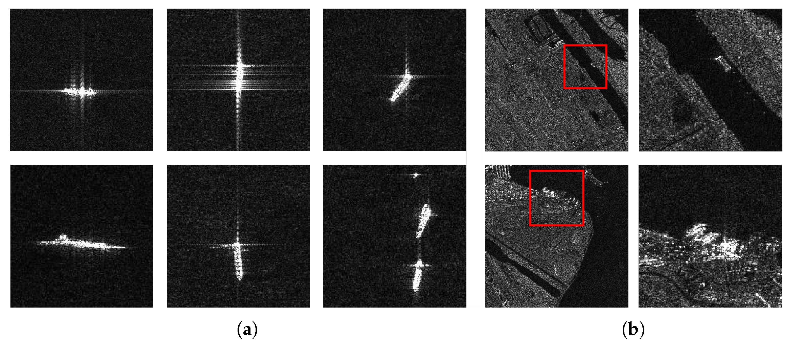
Meanwhile, different from objects in optical images that are rotation-invariant. Objects in SAR images do not share this property as we have observed variations in patterns of objects of relatively similar scales and aspect ratios, as is shown in Figure 1a and Figure 2. The characteristics of SAR objects require the learning of more effective representations. Moreover, as is shown in Figure 1b, ships are vulnerable to land clutters and sea clutters. Focusing only on the local features of ships and ignoring the relationship between image contexts makes it impossible to effectively attend to the semantic features of the image. Therefore, to deal with learning more effective representations and learning from image context at the same time, we propose the Orientation Enhancement Module (OEM) to enhance orientation-related information without redesigning the mechanism.

As is shown in Figure 5a, the OEM is an extension of the original MSDA by leveraging the Rotation-Sensitive convolution mechanism to capture orientation-related information for ships under different layout conditions and the self-attention mechanism to capture global pixel-wise dependencies. The OEM mainly consists of two parts: the Rotation-Sensitive convolution calculation and the channel-wise feature re-weighting with self-attention. In the first part, the Rotation-Sensitive Module (RSM) is used, with its structure shown in Figure 5b. It extracts rotation information using the Oriented Response Convolution [52], which calculates standard convolution feature maps with rotated convolution kernels of different angles. It also uses the ORPool operation to select maximum activation from ORConv calculations. In the second part, the self-attention calculations on channels are performed to adjust the original encoder memory sequence with the rotation-related information learned through the first stage.

Let $x_i\in {\mathbb{R}}^{C\times H\times W}$ be the i-th level of multi-scale feature maps and N be the number of orientation channels used in ORConv. We first get the output feature map ${\widehat{x}}_i$ with the Active Rotation Filter (ARF) F through standard convolution by:

$${\widehat{x}}_{i,n}=F_{{\theta }_n}(x_i),{\theta }_n=n\frac{2\pi }{N},n=0,1,\dots ,N-1$$

(5)

where $F_{{\theta }_n}(x_i)$ denotes applying ARF with rotation angle ${\theta }_n$ as convolution kernel on feature map $x_i$. Then, the ORPool operation is performed via max-pooling as:

$$x_{out,i}=ma{x}_n({\widehat{x}}_i)$$

(6)

After the extraction process of rotation-related information, for each layer, we perform channel-wise feature re-weighting by first applying self-attention calculation on $x_{out,i}$ as:

$$A_i=Softmax\{\frac{W_q{x}_{out,i}·{(W_k{x}_{out,i})}^T}{\sqrt{d}}\}·W_v{x}_{out,i}$$

(7)

where $W_q$, $W_k$ and $W_v$ are linear projection matrices, d is a constant value used as scale modulator of the product of q and k inputs. Then we concatenate attention weights from each layer and reduce the number of channels through fully connected networks as:

$${\widehat{s}}_{mem}=F_{align}([A_0,A_1,\dots A_{L-1}])·s_{mem}$$

(8)

where $s_{mem}$ denotes the encoder memory sequence and ${\widehat{s}}_{mem}$ denotes it after being processed. The $[·]$ operation denotes the channel-wise concatenation that yields a tensor with $L\times C$ channels given attention inputs from all L levels. $F_{align}$ is the fully connected sub-network that maps L attention weights with C channels to one vector with C channels.

Through these operations, OEM is designed to be a parallel re-weighting extension outside the encoder structure. OEM extracts Rotation-Sensitive attributes of SAR objects that are not present in the encoder sequence to initially highlight the targets. Then, it learns to enhance them, as well as suppressing irrelevant features in the background via multi-layer channel-wise re-weighting to render the represented objects more salient to downstream detector heads, leading to easier detection of these objects.

3.4. Grouped Relation Contrastive Loss

The Content De-noising mechanism is introduced to facilitate learning of more robust class prototypes and bounding-box representations. The collection of these class prototypes is called a label book in their implementations and consists of embedding vectors with quantities equal to the number of classes. Label book is used to initialize components of decoder input queries used in label de-noising. The label book is updated through backpropagation at each training iteration to acquire more representative class prototypes. However, as we further investigate this mechanism, we discovered two major issues:

• Class prototypes spontaneously become less discriminative as the training process goes on. (Values of Confusion Matrices rise as epoch number increases), as can be deduced from Figure 6a.
• Class prototypes have learned to adjust to better represent classes but have failed to learn to better discriminate between each other. When not back-propagating basic contrastive loss, we discovered natural descent on this loss value, as is shown in Figure 6a, but CM values still rise even when we add basic contrastive loss to explicitly designate distinctiveness as an optimization factor, as is changed in a similar way, like in Figure 6b.

Therefore, we conclude from the above that in the label de-noising part of the Content De-noising mechanism, the distinctiveness of class prototypes themselves is neglected. This imposes difficulties on the classification branch when the class A label is flipped as class B, but prototypes of class A and class B are similar. Since prototypes of class A and B are close to each other in vector space, the query corresponding to this prototype will not be correctly de-noised and the classification loss on this query will be undesirably low and wrongly propagated.

To better address the aforementioned issues, we seek to utilize both the intra-class and inter-class relationships of all class prototypes within the label book, in order to facilitate better representation learning of CDN mechanism. Considering the binary classification of the foreground class and the background class, we add additional representations called groups or patterns to better reserve different aspects of class features. When calculating relationships for groups, on the one hand, we seek to increase the distance with the most similar inter-class group so that representations that are most likely leading to confusions between the foreground and the background will be suppressed. On the other hand, we also seek to shrink the distance for least similar intra-class group so that the all groups responsible for the same category will learn to include confused features and to better separate them in feature space. To fulfill this purpose, we formulate our method as follows.

The original contrastive loss is first used in unsupervised learning and aims to facilitate learning of representations invariant to different views of the same instance by making positive pairs attracted and negative pairs separated. This loss can be formulated as:

$${\mathcal{L}}_{cr}(f,g)=-log\frac{exp(\frac{f_c·g_c^T}{\tau })}{exp(\frac{f_c·g_c^T}{\tau })+{\sum }_{k\ne c}exp(\frac{f_c·g_k^T}{\tau })}$$

(9)

where $f_c$ is a feature vector belonging to class at index c and $g_c$ is another class c vector which can be the same as $g_c$. In our case, we replace f to q to represent queries responsible for predictions, and g to b to represent label book embeddings that have the same number of feature dimensions as q. To apply contrastive loss on q of containing duplicated classes and b, the loss is formulated as:

$$\mathcal{L}(q,b)=-log\frac{{\sum }_{i}exp(\frac{q_{c,i}·b_c^T}{\tau })}{{\sum }_{i}exp(\frac{q_{c,i}·b_c^T}{\tau })+{\sum }_{k\ne c}exp(\frac{q_{c,i}·b_k^T}{\tau })}$$

(10)

where $q_{c,i}$ denotes the i-th vector of $q_c$. To address the aforementioned problem that representations in the label book failed to learn to distinguish themselves from each other, we add self-relation as a component of the total contrastive loss and we denote the total loss as:

$${\mathcal{L}}_{cr,total}(q,b)={\lambda }_{self}·{\mathcal{L}}_{cr}(q,q)+{\lambda }_{cross}·{\mathcal{L}}_{cr}(q,b)$$

(11)

We first observed a performance increase in the DOTA 1.0 dataset [53], which is an optical dataset that has a total of 15 classes, after applying Equation (11) as a loss term, while we also observed the desired effect of this initial loss, as is shown in Figure 6.

But ship detection in SAR images only recognizes objects as foreground objects or background which means significantly fewer classes. To deal with this issue, we direct our focus to intra-class variations, which is common in datasets with over-generalized classes. We discover in Figure 1a that pattern differences exist regardless of the ships’ orientation and background noise patterns are equally diverse, and the visual confusion between ships and background noises become more frequent in near-shore scenes, as is shown in Figure 1b. We conclude that considerable intra-class variations are present in both the foreground class and the background class, and hence it is natural to modify this loss to enable multiple representations for each class.

Given number of patterns per class as K, we have the expanded label book $b\in {\mathbb{R}}^{N_c\times K\times C}$, where $N_c$ is the total number of classes. Now, given queries $q\in {\mathbb{R}}^{N_q\times C}$, we first normalize by:

$${\widehat{q}}_c·{\widehat{b}}_g^T=\frac{q_c·b_g^T}{\Vert q_c{\Vert }_2·{\Vert b_c\Vert }_2}$$

(12)

We calculate similarities of the intra-class representations of the g-th group $S(q_c,b_{g,c})$ by:

$$S(q_c,b_{g,c})=\underset{i}{max}[exp(\frac{{\widehat{q}}_{c,i}·{\widehat{b}}_{g,c}^T}{\tau })]$$

(13)

which means selecting the least discriminative representation of a different class to enlarge the distance between compared C-dimensional vectors. Discrepancies of inter-class representations $D(q_c,b_{g,\widehat{c}})$ are calculated as:

$$D(q_c,b_{g,\widehat{c}})=\underset{i}{min}[exp(\frac{{\widehat{q}}_{c,i}·{\widehat{b}}_{g,\widehat{c}}^T}{\tau })]$$

(14)

where $\widehat{c}$ denotes any single class that is not class c. It means shrinking the distance between the most discriminative representation of the same class and the current vector. We do the same for self-relations among grouped representations and hence formulated the Relational Loss (RL) term as:

$${\mathcal{L}}_{RL}(q,b)=-log\frac{{\sum }_{c}S(q_c,b_{g,c})}{{\sum }_{c}S(q_c,b_{g,c})+{\sum }_{\widehat{c}}D(q_c,b_{g,\widehat{c}})}$$

(15)

Hence, we obtain the total Grouped Relation Contrastive Loss (GRC Loss) as:

$${\mathcal{L}}_{GRC}(q,b)={\lambda }_{self}·{\mathcal{L}}_{RL}(q,q)+{\lambda }_{cross}·{\mathcal{L}}_{RL}(q,b)$$

(16)

The whole process of training with GRC Loss is shown in Algorithm 1. The algorithm isolates calculations between matched queries and each group of representations from matched queries themselves or the label book.

Algorithm 1: Training with GRC Loss

Require: Queries from Encoder $q_e\in {\mathbb{R}}^{{\sum }_i{H}_i·W_i\times C}$, classification scores of each query $q_{e,cls}$, Label book $b\in {\mathbb{R}}^{N_c·K\times C}$, predictions of model $preds$, number of encoder queries to be selected $N_q$, number of classes $N_c$, number of patterns in each group K   1: Get sorted scores = sort ($q_{e,cls}$, order = descend, dimension = last)   2: Get sorted $q_e$ = sort ($q_e$) with sorted scores   3: Get selected queries q = collect (sorted $q_e$, amount = $N_q$), with number of queries N   4: Get matched labels L = Hungarian Assignment ($preds$, ground-truths)   5: Get normalized self-relations $C_{self}$ and cross-relations $C_{cross}$ by Equation (12)   6: Set numerator A and denominator B to zero   7: for b is label book b or selected queries q do   8:    for $g=1$ to $N_c$ do   9:      Generate binary mask $M_{cross,g}\in {\mathbb{R}}^{N\times K}$, where $L_g=g$ is 1, otherwise 0 10:      Do the same as above to get $M_{self,g}\in {\mathbb{R}}^{N\times K}$ 11:      Select $C_{self,g}$ with mask $M_{self,g}$ and $C_{cross,g}$ with $M_{cross,g}$ 12:      Calculate $S(q_c,b_g)$ and $D(q_g,b_{\widehat{g}})$ with Equations (13) and (14) 13:      Add $S(q_c,b_g)$ to A and $D(q_g,b_{\widehat{g}})$ to B 14:    end for 15:    Calculate ${\mathcal{L}}_{RL}$ with $-log[\frac{A}{A+B}]$ 16:    Add $\lambda ·{\mathcal{L}}_{RL}$ to total loss ${\mathcal{L}}_{GRC}$ 17: end for 18: Return ${\mathcal{L}}_{GRC}$

For a more intuitive view of the entire loss, we present in Figure 7 calculations of GRC Loss with two classes with a pattern number of three and four matched queries. Each color represents the mask generated for each class of a group. Tiles with darker colors represent relation values selected by the $min/max$ function in Equations (13) and (14). Therefore, calculations for each group are isolated from each other but are parallel for each type of query within the group. Our GRC Loss achieved the desired effect in our initial DOTA test, as is shown in Figure 6c, and we will further discuss its effects on SAR objects and internal attributes in Section 4 and Section 5.

4. Experiments

4.1. Datasets

Our method is developed to accommodate object detection tasks for objects like ships and vehicles in SAR images. To validate the effectiveness of our proposed methods, we conduct experiments on two public datasets, the High-Resolution SAR Image Dataset (HRSID) [43] and the SAR Ship Detection Dataset (SSDD) [44]. We also conduct experiments on the SAR Vehicle Dataset, which is developed by us, to evaluate the performance of vehicle objects.

• HRSID: The HRSID dataset was constructed by SAR images from the Sentinel-1B, TerraSAR-X, and TanDEM-X satellites. It contains 5604 high-resolution SAR images of $800\times 800$ in size and a total of 16,951 ships with multiple scales; 65% of the dataset is divided as the training set and the rest as the test set. The format of annotation follows MS-COCO [51] standards, including areas and bounding boxes (x, y, width, height) where x and y represent the coordinates of the top-left corner of the annotation bounding box. We follow MS-COCO evaluation standards to determine small ships, medium ships, and large ships. Ships with bounding box areas below $32\times 32$ pixels are marked as small, areas between $32\times 32$ and $96\times 96$ as medium, and areas over $96\times 96$ as large. Small, medium, and large ships account for 54.5%, 43.5%, and 2% of all annotated ships.
• SSDD: The images of SSDD are acquired by RadarSat-2, TerraSAR-X, and Sentinel-1 satellites, with four polarization modes of HH, HV, VV, and VH. It consists of 1160 SAR images with a resolution of 1–15 m of different sizes, such as $416\times 323$ and $501\times 355$. The train set consists of 928 images, and the test set has 232 images. There are 2551 ships in total; 1463 are small ships, 989 are medium ships, and 99 are large ships.
• SAR Vehicle Dataset: Targets in SAR images commonly appear as ships and vehicles. As we have tested our method on ship datasets, it is also essential to include the evaluation of vehicles in our experiments. Our dataset currently consists of 440 labeled images, and 1876 labeled vehicle instances featuring multi-scale urban scenes and different noise conditions. We are still expanding this dataset. We apply an 8/2 split ratio for the train set and the test set. Samples are processed from raw complex data of FARAD X Band, Ka-Band, Spotlight SAR, and Mini SAR imagery, with each cropped as 800 × 800 patches. Vehicles in these images have various scales and noise conditions. We follow the standard MS-COCO annotation format to store horizontal box annotations. Small, medium, and large vehicles by MS-COCO standards account for 21.7%, 78.1%, and 0.2% of all labeled objects, respectively.

Samples of both datasets are shown in Figure 8. Both datasets feature objects under various scenes. For ship objects in Figure 8a,b, variations in scenes fall in offshore and inshore categories. For vehicle objects, appearances resemble inshore ships but the challenges of detecting these objects are mostly brought by foliage coverage and distractions of nearby buildings.

4.2. Implementation Details

The backbone network of our experiments is an ImageNet pre-trained ResNet-50 network and we used nothing other than each dataset itself to train and validate our methods. Multi-scale feature maps are extracted from $con{v}_3$ to $con{v}_5$ of the ResNet-50 backbone. The base number of queries is set to 900 and the de-noising number is set to 100, with label noise scale at 0.5, box noise scale at 1.0. We train the model for 12 and 20 epochs and other compared methods for 20 epochs on HRSID, where we achieved optimal performance at 20 epochs. We trained our method and other compared methods for 100 epochs on the SSDD dataset considering the scale and our method did not converge at the 12th epoch, so we continued the training. For every setting, we start the learning rate at $1\times {10}^{-4}$ with weight decay at $1\times {10}^{-4}$ on the AdamW optimizer, the learning rate descends to $1\times {10}^{-5}$ at the 11th epoch. Training data augmentations are used, and during training, we apply random resizing and random flipping, and during test time we use resizing only to match up the input shape of compared CNN-based methods. In all ablation studies, we adopt Deformable DETR with the CDN mechanism as our baseline method. For OEM, we set the number of Rotation-Sensitive blocks to three. For GRC Loss, we set total loss weight at 2.0, ${\lambda }_{self}=1.2$, ${\lambda }_{cross}=0.5$, $\tau =2$, and label book pattern number $K=3$. Other than GRC Loss, losses we have used are focal loss on classification, with $\alpha =0.25$, $\gamma =2.0$. L1 and GIOU loss are used on bounding-box regression. We set loss weights for the above losses at 1, 5, and 2, respectively. The cost weights of these losses for the Hungarian matcher are the same as the loss weights. The batch size is set to two and we apply distributed training on two GeForce RTX 3090 GPUs. All experiments are conducted on the Linux platform, 18.04 LTS. The model and its components are implemented under the MMDetection and Pytorch framework.

4.3. Evaluation Metrics

In this article, we calculate Precision and Recall with Equations (17) and (18) by VOC metrics [54], as are in other related works. $TP$ suggests true positives which are correctly predicted foreground objects. $FP$ suggests false positives which are background noises wrongly predicted as foreground objects, and $FN$ are false negatives that are missed foreground objects. The F1 score is the harmonic mean of Precision and Recall, defined as Equation (19). $AP$ denotes Average Precision, which is the area under the Precision–Recall curve. It is defined as Equation (20) and approximated by Equation (21). Precision and Recall terms are calculated when an Intersection over Union (IOU) threshold with ground-truth objects is given. For experiments on SSDD, we adopt Precision, Recall, and AP under an IOU threshold of 0.5 for comparison with other methods.

$$Precision=\frac{N_{TP}}{N_{TP}+N_{FP}}$$

(17)

$$Recall=\frac{N_{TP}}{N_{TP}+N_{TN}}$$

(18)

$$F1=\frac{2\times Precision\times Recall}{Precision+Recall}$$

(19)

$$AP={\int }_0^{1}P(r)dr$$

(20)

$$AP=\frac{1}{101}\sum _{i=0}^{100}{Precision|}_{Recall=0.01i}$$

(21)

For experiments on the HRSID dataset, we follow MS-COCO definitions and adopt $mAP$, $A{P}_{50}$, $A{P}_{75}$, $A{P}_S$, $A{P}_M$, and $A{P}_L$ as evaluation metrics. $A{P}_{50}$ and $A{P}_{75}$ denote average precision under IoU thresholds of 0.5 and 0.75, respectively. $mAP$ denotes the average precision yielded under different IoU thresholds from 0.5 to 0.95 with a constant step of 0.05. $A{P}_S$, $A{P}_M$, and $A{P}_L$ evaluate the detection performance on small, medium, and large ships, respectively.

Among all used metrics, we prioritize F1 as the major performance indicator as it is a balanced factor to evaluate both the distinguishability and accuracy of a detection method. In cases that do not require Precision or Recall in VOC metrics, we follow MS-COCO standards and prioritize $mAP$.

4.4. Ablation Study and Model Analysis

In all sets of ablation experiments, we use the Deformable DETR with the CDN mechanism attached as the baseline for comparisons. For each set of ablation experiments, we repeat with three different sets of random seeds to avoid accidental results and collect the means and standard deviations for each type of experiment, respectively. Results for all experiments are shown in the both

Table 1. Ablation experiments for Orientation Enhancement Module (OEM).

Method	Nepoch	Seed No.	mAP	AP50	AP75	APS	APM	APL
baseline	12	1	0.613	0.866	0.698	0.635	0.619	0.259
baseline	12	2	0.611	0.868	0.706	0.633	0.597	0.229
baseline	12	3	0.614	0.871	0.713	0.637	0.601	0.247
baseline + OEM	12	1	0.62	0.884	0.713	0.638	0.615	0.248
baseline + OEM	12	2	0.624	0.883	0.722	0.644	0.612	0.254
baseline + OEM	12	3	0.623	0.882	0.718	0.642	0.611	0.277
baseline	12	all	0.613 (±0.002)	0.868 (±0.003)	0.706 (±0.008)	0.635 (±0.002)	0.606 (±0.012)	0.245 (±0.015)
baseline + OEM	12	all	0.622 (±0.002)	0.883 (±0.001)	0.718 (±0.005)	0.641 (±0.003)	0.613 (±0.002)	0.260 (±0.015)
baseline	20	1	0.629	0.884	0.723	0.651	0.628	0.305
baseline	20	2	0.623	0.885	0.721	0.645	0.611	0.269
baseline	20	3	0.628	0.894	0.723	0.647	0.619	0.269
baseline + OEM	20	1	0.637	0.897	0.732	0.653	0.634	0.327
baseline + OEM	20	2	0.632	0.889	0.731	0.651	0.61	0.312
baseline + OEM	20	3	0.633	0.894	0.729	0.655	0.606	0.309
baseline	20	all	0.627 (±0.003)	0.888 (±0.006)	0.722 (±0.001)	0.648 (±0.003)	0.619 (±0.009)	0.281 (±0.021)
baseline + OEM	20	all	0.634 (±0.003)	0.893 (±0.004)	0.731 (±0.002)	0.653 (±0.002)	0.617 (±0.015)	0.316 (±0.010)

and

Table 2. Ablation experiments for Grouped Relation Contrastive (GRC) Loss.

Method	Nepoch	Seed No.	mAP	AP50	AP75	APS	APM	APL
baseline + GRC	12	1	0.613	0.866	0.698	0.635	0.619	0.259
baseline + GRC	12	2	0.614	0.868	0.7	0.628	0.599	0.254
baseline + GRC	12	3	0.613	0.87	0.709	0.637	0.605	0.189
baseline	12	all	0.613 (±0.002)	0.868 (±0.003)	0.706 (±0.008)	0.635 (±0.00)	0.606 (±0.012)	0.245 (±0.015)
baseline + GRC	12	all	0.613 (±0.001)	0.868 (±0.002)	0.702 (±0.006)	0.633 (±0.005)	0.608 (±0.010)	0.234 (±0.039)
baseline + GRC	20	1	0.634	0.887	0.729	0.652	0.625	0.289
baseline + GRC	20	2	0.628	0.886	0.727	0.648	0.617	0.299
baseline + GRC	20	3	0.632	0.89	0.724	0.654	0.612	0.279
baseline	20	all	0.627 (±0.003)	0.888 (±0.006)	0.722 (±0.001)	0.648 (±0.003)	0.619 (±0.009)	0.281 (±0.021)
baseline + GRC	20	all	0.631 (±0.003)	0.888 (±0.002)	0.727 (±0.003)	0.651 (±0.003)	0.618 (±0.007)	0.289 (±0.010)

. Means and deviations are shown in the “Mean (±Std.)” format.

4.4.1. Effect Analysis on OEM

OEM is proposed to integrate rotation-related information into the feature memory sequence after encoder calculation. To verify the effect of OEM, we test OEM on the HRSID dataset and compare it with the baseline at 12 and 20 epochs and itself at 20 epochs. We still follow the same evaluation metrics in comparison. As Table 1 shows, compared with baseline, OEM increased $1.8\%$ and $1.5\%$ at $A{P}_{50}$ and $A{P}_{75}$, respectively, at 12 epochs and increased $0.7\%$ and $0.9\%$ at 20 epochs. This is because rotation-related features for ships are distinct and necessary for recognizing ships in different rotated conditions and OEM is designed to acquire such features.

4.4.2. Effect Analysis on GRC Loss

The GRC Loss term is designed to emphasize intra-class variations that were neglected in the over-generalized foreground classification and inter-class differences. To verify the effect of GRC Loss, we use the same metrics and HRSID dataset and set the number of patterns per group K to 3, ${\lambda }_{self}$ to 1.2, ${\lambda }_{cross}$ to 0.8 and the temperature factor $\tau$ to 2, to compare with baseline at 12 and 20 epochs and itself at 20 epochs. Results are shown in Table 2.

To further study the impact of K on the performance of our method, we tested a set of different K values on the HRSID dataset with training epochs at 12 and 20 epochs, shown in

Table 3. Impact of K value in GRC Loss.

Setting of K	Nepoch	mAP	AP50	AP75	APS	APM	APL
K = 1	12	0.611	0.868	0.706	0.633	0.597	0.229
K = 2	12	0.61	0.87	0.704	0.633	0.592	0.221
K = 3	12	0.613	0.869	0.708	0.637	0.603	0.234
K = 4	12	0.611	0.87	0.707	0.633	0.587	0.227
K = 1	20	0.623	0.885	0.721	0.645	0.611	0.269
K = 2	20	0.627	0.887	0.722	0.65	0.616	0.272
K = 3	20	0.634	0.887	0.729	0.652	0.625	0.289
K = 4	20	0.628	0.887	0.725	0.648	0.618	0.312

Bold: Highest value of each column.

.

4.5. Comparison Experiments

To further validate the performance of our proposed method, we compare with a set of different detection methods, including FoveaBox [55], Yolact [56], Faster R-CNN [57], PAFPN [58] on Faster R-CNN, YOLOv3 [59], RetinaNet [60], Libra R-CNN [61], and FCOS [62]. As well as CNN-based methods, we also draw comparisons with DETR series models, such as DAB-DETR [29], which is the latest derivation of dense-sampling DETR, and Deformable DETR [27]. In

Table 4. Comparison experiments on HRSID dataset.

Method	mAP	AP50	AP75	APS	APM	APL
DAB-DETR	-	-	-	-	-	-
SSD	0.47	0.744	0.523	0.47	0.622	0.26
Defm. DETR	0.48	0.793	0.532	0.494	0.455	0.039
NAS-FPN	0.517	0.763	0.565	0.51	0.652	0.217
YOLOv3	0.536	0.862	0.573	0.534	0.606	0.266
Fstr. R-CNN	0.537	0.767	0.599	0.539	0.604	0.129
FCOS	0.549	0.805	0.613	0.563	0.575	0.092
RetinaNet	0.582	0.83	0.644	0.592	0.624	0.25
Libra R-CNN	0.603	0.799	0.696	0.609	0.649	0.226
PAFPN	0.603	0.806	0.691	0.606	0.668	0.329
FEM + ICM [7]	0.606	0.855	0.679	0.614	0.655	0.32
FINet [6]	0.613	0.886	0.698	0.635	0.619	0.259
baseline (E12)	0.613	0.866	0.698	0.635	0.619	0.259
baseline (E20)	0.629	0.884	0.723	0.651	0.628	0.305
Ours (E12)	0.626	0.886	0.719	0.647	0.606	0.238
Ours (E20)	0.649	0.905	0.744	0.667	0.626	0.341

“-”: Results not available due to no convergence. Bold: Highest value of each column.

, our proposed method achieved the highest performance in almost every metric although having slightly inferior performance on predicting medium-sized targets compared with methods with close $mAP$. Moreover, DAB-DETR as a single-scale dense-sampling DETR model failed to converge during training, and Deformable DETR performed worse than almost every other CNN-based method.

To validate the effectiveness of our method and also to line up with other related works, we have also drawn comparisons between our method and other SAR ship-detection-related methods on the SSDD dataset. We adopt Precision and Recall as most commonly used in other works. Though we train our method for a relatively longer duration, we still evaluate and compare at the 12th epoch to provide additional comparisons to line up with the settings of Hu et al. [6]. From

Table 5. Comparison experiments for SSDD dataset.

Method	F1	Precision	Recall	AP50	AP75
DAB-DETR	-	-	-	-	-
Yolact	0.408	0.357	0.476	0.871	0.179
YOLOv3	0.598	0.563	0.637	0.877	0.407
RetinaNet	0.734	0.709	0.761	0.885	0.789
Fstr. R-CNN	0.746	0.725	0.768	0.907	0.832
CRCN 1 [63]	0.755	0.738	0.775	0.896	0.781
HRSD 2 [64]	0.756	0.743	0.786	0.897	0.816
FCOS	0.806	0.722	0.912	0.736	0.371
Defm. DETR	0.832	0.733	0.962	0.750	0.457
Ours (E12)	0.926	0.87	0.989	0.826	0.685
Ours	0.936	0.89	0.987	0.939	0.840

“-”: Results not available due to no convergence. ¹: Abbreviation for Cascade R-CNN. ²: Abbreviation for HR-SDNet. Bold: Highest value of each column.

, we can find that our method surpasses other methods by a fair margin concerning the F1 score. And among DETR methods, DAB-DETR still does not converge during training. Although Deformable DETR achieved the best Precision, its low Recall rate suggests that it missed too many objects. While the Recall rate at the 12th epoch is higher than that of the 20th epoch by 1%, our method at the 20th epoch regains 2% increase in Precision, leading to a 1% increase in the F1 score with an acceptable trade-off with Recall.

Vehicles, as well as ships, fall in the common object categories of SAR images. Ships typically appear in offshore and nearshore settings, where in the latter case, detection becomes notably more challenging due to the requirement of representing objects and reducing background noise, particularly in areas with concentrated buildings. To validate that our method works on both ships and vehicles, we draw another comparison experiment on our publicly released SAR vehicle dataset. Experiment settings follow those in previous experiments, and all methods are trained for 20 and 50 epochs.

From

Table 6. Comparison experiments for SAR Vehicle Dataset.

Method	Nepoch	F1	Precision	Recall	AP50	AP75	mAR
FoveaBox	-	-	-	-	-	-	-
Yolact	-	-	-	-	-	-	-
DAB-DETR	-	-	-	-	-	-	-
FCOS	-	-	-	-	-	-	-
RetinaNet	-	-	-	-	-	-	-
Defm. DETR	20	0.279	0.247	0.708	0.2	0.03	0.321
YOLOv3	20	0.370	0.465	0.705	0.46	0.091	0.307
PAFPN	20	0.424	0.501	0.681	0.491	0.221	0.368
Casc. R-CNN	20	0.431	0.497	0.698	0.5	0.225	0.38
Ours	20	0.440	0.374	0.895	0.359	0.145	0.535
Libra R-CNN	20	0.448	0.493	0.79	0.503	0.187	0.41
Fstr. R-CNN	20	0.526	0.492	0.651	0.345	0.136	0.565
Defm. DETR	50	-	-	-	-	-	-
YOLOv3	50	0.323	0.413	0.597	0.399	0.07	0.265
PAFPN	50	0.368	0.445	0.58	0.444	0.176	0.313
Fstr. R-CNN	50	0.369	0.454	0.566	0.469	0.19	0.311
Casc. R-CNN	50	0.375	0.46	0.573	0.451	0.188	0.316
Libra R-CNN	50	0.400	0.471	0.664	0.477	0.176	0.348
Ours	50	0.470	0.402	0.936	0.396	0.153	0.565

“-”: Results not available due to no convergence. Bold: Highest value of each column.

, we can find that some methods that worked in ship detection scenarios failed to converge during training, and our method surpasses other Transformer-based methods by a fair margin. We also find that as training duration extends, every CNN-based method has overfitted the vehicle dataset. CNN-based methods reach their peak performance at the 20th epoch but drop significantly at the 50th epoch, whereas the performance of our method continuously increases. Moreover, decreases in Recall rates of CNN-based methods indicate that these methods are gradually confused by training samples and misinterpreted as background noises. The relatively slight decreases in Precision suggest that CNN-based methods have still learned accurate predictions of several distinguishable targets. Although our method did not achieve the best detection Precision in this experiment, the significantly high Recall rate of our method suggests that even if our method predicts less accurate bounding boxes, it is hardly confused by background noises and has the ability to distinguish underlying objects. This proves that our method has a huge learning capacity, excellent detection performance, and flexibility under both simple and complex detection conditions.

4.6. Generalization Experiment

In addition to performance, we also conducted a migration test following Hu et al. [5]. We first train our method on the HRSID dataset that yields the optimal evaluation results shown in Table 4. Then, we directly enter inference mode on the SSDD dataset to obtain test results. We pick $A{P}_{50}$, $A{P}_{75}$, Precision, Recall, and F1 because these metrics are used in their experiment.

Based on results from Table 5 and

Table 7. Migration experiments for SSDD dataset.

Method	F1	AP50	AP75	Precision	Recall
DAB-DETR	-	-	-	-	-
Fstr. R-CNN	0.234	0.625	0.054	0.189	0.308
HRSD 1 [64]	0.246	0.632	0.062	0.196	0.329
FoveaBox	0.255	0.626	0.054	0.206	0.333
FCOS	0.257	0.607	0.091	0.216	0.318
CRCN 2 [63]	0.277	0.637	0.086	0.222	0.369
PAFPN	0.285	0.35	0.091	0.197	0.435
YOLOv3	0.291	0.678	0.104	0.245	0.358
BANet [5]	0.294	0.673	0.113	0.251	0.355
Defm. DETR	0.326	0.598	0.157	0.242	0.498
Libra R-CNN	0.385	0.41	0.09	0.316	0.491
baseline	0.406	0.665	0.307	0.335	0.515
Ours	0.412	0.696	0.278	0.333	0.540

“-”: Results not available due to no convergence. ¹: Abbreviation for HR-SDNet. ²: Abbreviation for Cascade R-CNN. Bold: Highest value of each column.

, we can find that performance for every tested method has dropped significantly. Among them, we find that two-stage detectors generally perform better than single-stage counterparts during training, but they show a lack of generalization ability in the migration test. In this experiment, the performance of our method has also dropped but still shows the best performance. This means that our method learns more effective representations of different ship patterns in SAR images without having to rely on handcrafted priors for feature processing. Secondly, although Precision and $A{P}_{75}$ have dropped, increase in $A{P}_{50}$, Recall, and most importantly the F1 score indicates that with our proposed method, we miss fewer objects via an acceptable trade-off with accuracy. At last, as we compare among DETR based methods in both Table 5 and Table 7, we can find that dense-sampling DETRs like DAB-DETR are not suitable for detection in SAR images, and sparse-sampling DETRs like Deformable DETR are compatible to the task, though they still need specialized improvements to catch up with CNN-based methods.

4.7. Visualization

To verify the performance of our method, we visualize randomly selected samples in both offshore, inshore, and land scenarios from all datasets we have used, as can be seen in Figure 9. These scenarios are typical for SAR object detection and current applications in maritime surveillance and road safety, and our method in general shows satisfactory detection performance under various conditions.

Additionally, to better identify underlying reasons for the improved performance of our proposed method compared to others, we select YOLOv3 and FCOS model representing single-stage detectors and Libra R-CNN and PAFPN representing two-stage detectors for visualization. We select four sample images from the HRSID dataset, ranging from offshore scenes to near shore or land scenes since such order indicates an increase in noise diversity and also difficulty in detection. We discuss the performances of compared methods on off-shore and near-shore scenes, each of which contains two sample images. Red boxes denote predicted boxes. For better interpretation, we mark areas to be noted with yellow boxes. We additionally apply zooming to some of the yellow boxes and their paired green boxes of the corresponding ground-truth areas. We provide ground-truth images of used vehicle samples since the construction of our dataset is still in progress.

4.7.1. Off-Shore Scenes

In Figure 10a, which is the simplest of all, our method and single-stage detectors correctly predict the actual bounding boxes of the ships. However, two-stage detectors fail on the right-side ship with duplicated predictions. In Figure 10b, we find inaccurate predictions of the middle- and upper-side-ship by YOLOv3 and FCOS, respectively. FCOS and Libra R-CNN have incorrectly detected background noises around the harbor as ships, and PAFPN predicts duplicated ships, as is similar in Figure 10a. Our method is not found to have these issues and has predicted the correct bounding boxes.

4.7.2. Nearshore Scenes

In Figure 11a, we find that apart from our method and FCOS, other methods have incorrectly detected land clutters near harbors as ships to different extents. Libra R-CNN detects the most false positives while also detecting part of the land area in the upper-right part as a ship. PAFPN and YOLOv3 confuse the small sea clutter in the upper-left quarter as a ship. In Figure 11b, we can find that two-stage detectors detect false positives in the bottom part more often. Single-stage detectors though make many fewer mistakes, and they miss the ship on the left part. FCOS in comparison with YOLOv3 is significantly less confident with its predictions despite being equally accurate.

Combined with the observations made in Figure 10a,b, we can assume that two-stage detectors have relatively poor generalization ability on small objects. As is shown in Table 7, most two-stage networks suffered a more significant performance drop on the migration experiments in terms of F1 scores, while single-stage networks showed a relatively mild performance drop, and we can be more assured to conclude that two-stage networks have a tendency to overfit dataset-specific features as shortcuts for better detection performance. The FCOS network, which ranked second in performance on the SSDD dataset, collapsed on the migration experiment. We assume that this is because the miniature architecture of the FCOS network has resulted in the overfitting problem.

However, in both cases our method not only makes no wrong or missed predictions but also detects every ship object with accuracy. Therefore, we conclude that our method is suitable for both off-shore and nearshore prediction and can maintain its superior performance in different datasets.

4.7.3. Vehicles

In Figure 12 and Figure 13, we display two typical detection scenes for our SAR Vehicle Dataset. As can be seen from Figure 12, in an open-field scenario, YOLOv3 and Cascade R-CNN fail to detect any instance. Libra R-CNN misinterprets the scale of the vehicle and falsely detects a background noise spot. PAFPN detects the instance though, and it still yields a false detection of a nearby lighting. And from Figure 13, where vehicles are near or hidden under foliage, YOLOv3 fails to recognize any instance, and Cascade R-CNN, PAFPN, and Libra R-CNN falsely detect a noise reflection on the rooftop in the bottom-left corner, whereas PAFPN successfully detects a target near the center. Our method in these cases not only shows an excellent ability to recognize objects, but it also correctly detects foliage-covered targets in Figure 13. Therefore, we conclude that our method not only has superior detection performance in ship detection but also has a competitive ability to detect vehicle instances in challenging conditions and is hence suitable to meet up with the task of detecting various targets.

5. Discussion

In this section, we discuss the effects of the OEM and the GRC Loss in the detection of SAR objects. In order to illustrate the effect of OEM more intuitively, we forward an image to models in the above settings to plot the differences between the enhanced feature memory sequence and the original feature memory sequence and also display the input image shown in Figure 14.

It can be observed that edge features of the oriented ships have been initially enhanced by the Rotation-Sensitive Module as shown in the third columns of Figure 14a,b, whereas this effect is not observed in the direct output of the FPN network. Then the OEM module focuses on object-related features and suppresses irrelevant features with self-attention, as we can observe in the last columns of all sample images.

To also further demonstrate the function of GRC Loss and verify if it meets the designed purposes, we visualize the effect of GRC Loss during training. As for the design purpose of GRC Loss, it aims to alleviate the over-generalization problem with SAR object classification by introducing variations within classes while also reducing confusion with object-like background noises. We apply tSNE to output queries collected after 20 iterations under different settings. We additionally draw the contour lines of tSNE point density to more intuitively visualize the location and clustering pattern of foreground queries.

As can be observed from the second row of Figure 15, the optimal GRC Loss settings of our method produce densely clustered foreground queries with a few located at the other edge of the blob. This indicates that foreground queries possess different focuses in the vector space and are easily distinguished from the majority of background noises. In the first row of Figure 15, foreground queries span across the blob in a way similar to that of the second row. At the early stages of training, foreground queries still show a greater clustering tendency compared to that of the first row. Moreover, as the third row suggests, foreground queries tend to scatter as the parameter K becomes larger than the optimal setting. We can additionally deduce from the above that parameter K in GRC Loss has a significant impact comparable to many epochs of training. For a more intuitive view of the effect of parameter K in GRC Loss, we also calculate and visualize numerical differences of confusion matrices of label books under different K settings. We use blue to denote value decrease and red for the increase.

In Figure 16, we find that distances of groups belonging to different classes are enlarged while distances of groups of the same class shrank. In Figure 16c, although we find that distances between some groups in different classes are brought closer, we still find a significant distance increase or value decrease for every pair of groups that belong to different master classes. In this case, Group 1 of the FG class has the least confusion with Group 1 of the BG class, and Group 2 of the FG class has the least confusion with Group 3 of the BG class, and Group 3 of the FG class has the least confusion with Group 2 of the BG class. Since we do not observe groups of the FG class and the BG class always find their least confused counterpart in the top-left to bottom-right diagonal line of each quarter, we can safely conclude that it is effective to implement contrastive loss in a grouped way so that each group can back up different information for their master classes.

Based on our conducted experiments, our method demonstrates superior performance in multi-scale detection within SAR images under various conditions. This success primarily stems from two key factors. Firstly, the high learning capacity of DETR plays a crucial role. Its effective representations for SAR objects effectively bridges the gap between DETR, initially designed for optical detection, and our proposed adaptation for SAR detection. However, this high learning capacity mainly results from DETR’s substantial parameter count, enabling recognition of objects in diverse, complex scenarios. Yet, this advantage comes at the expense of extensive computational runtime, limiting the incorporation of more enriched object representations into the network. Regarding the proposed modules, optimizing OEM involves reducing computation costs while retaining rich representations of rotation-related characteristics for SAR objects. On the other hand, enhancing the GRC Loss mechanism entails expanding the grouping approach to accommodate more enriched class representations and auxiliary prototypes in the label book. Moreover, introducing new auxiliary tasks related to SAR object characteristics into the CDN mechanism can significantly contribute to augmenting the GRC Loss method. These strategies are essential in advancing the framework by focusing on the efficacy of object representations, and eventually increasing performance in SAR object detection.

6. Conclusions

In this article, we propose specialized data enhancement and training modules for target detection in SAR images, which is the first method in this field that implemented the DETR framework, a Transformer-based object detection framework that utilizes sparse queries instead of pixel-wise dense predictions to retrieve task information. The OEM module applies self-attention on orientation-related features to incorporate orientation information into the feature memory sequence, enabling the model to better generalize object representations in different oriented conditions. The GRC Loss term enables the model to learn additional representations for intra-class variations while simultaneously dealing with the consistency of intra-class representations and the discrepancy of inter-class representations. The performance and generalization ability exhibited by Transformer framework through our design and experiments have proven that the Transformer is still competent in object detection outside optical contexts. And by bridging the Transformer to SAR images, we also open a feasible direction for future studies to further explore the capability of the Transformer framework in SAR images.

In the future, we will seek to develop SAR object representation methods with better detection ability and explainability based on the Transformer framework as well as developments on our SAR Vehicle Dataset. On the other hand, we will also look into the Transformer framework applied on oriented object detection in SAR images.

References

1. Liang, Y.; Sun, K.; Zeng, Y.; Li, G.; Xing, M. An adaptive hierarchical detection method for ship targets in high-resolution SAR images. Remote Sens. 2020, 12, 303. [Google Scholar] [CrossRef]
2. Du, L.; Li, L.; Wei, D.; Mao, J. Saliency-guided single shot multibox detector for target detection in SAR images. IEEE Trans. Geosci. Remote Sens. 2019, 58, 3366–3376. [Google Scholar] [CrossRef]
3. Ma, X.; Hou, S.; Wang, Y.; Wang, J.; Wang, H. Multiscale and dense ship detection in SAR images based on key-point estimation and attention mechanism. IEEE Trans. Geosci. Remote Sens. 2022, 60, 5221111. [Google Scholar] [CrossRef]
4. Cui, Z.; Wang, X.; Liu, N.; Cao, Z.; Yang, J. Ship Detection in Large-Scale SAR Images Via Spatial Shuffle-Group Enhance Attention. IEEE Trans. Geosci. Remote Sens. 2021, 59, 379–391. [Google Scholar] [CrossRef]
5. Hu, Q.; Hu, S.; Liu, S. BANet: A balance attention network for anchor-free ship detection in SAR images. IEEE Trans. Geosci. Remote Sens. 2022, 60, 5222212. [Google Scholar] [CrossRef]
6. Hu, Q.; Hu, S.; Liu, S.; Xu, S.; Zhang, Y.D. FINet: A Feature Interaction Network for SAR Ship Object-Level and Pixel-Level Detection. IEEE Trans. Geosci. Remote Sens. 2022, 60, 5239215. [Google Scholar] [CrossRef]
7. Zhu, M.; Hu, G.; Zhou, H.; Wang, S. Multiscale ship detection method in SAR images based on information compensation and feature enhancement. IEEE Trans. Geosci. Remote Sens. 2022, 60, 5117913. [Google Scholar] [CrossRef]
8. Kang, M.; Leng, X.; Lin, Z.; Ji, K. A modified faster R-CNN based on CFAR algorithm for SAR ship detection. In Proceedings of the Remote Sensing with Intelligent Processing, Shanghai, China, 19–21 May 2017; pp. 1–4. [Google Scholar]
9. Li, J.; Qu, C.; Shao, J. Ship detection in SAR images based on an improved faster R-CNN. In Proceedings of the SAR in Big Data Era: Models, Methods and Applications (BIGSARDATA), Beijing, China, 13–14 November 2017; pp. 1–6. [Google Scholar]
10. Lin, Z.; Ji, K.; Leng, X.; Kuang, G. Squeeze and excitation rank faster R-CNN for ship detection in SAR images. IEEE Geosci. Remote Sens. Lett. 2018, 16, 751–755. [Google Scholar] [CrossRef]
11. Zhao, Y.; Zhao, L.; Xiong, B.; Kuang, G. Attention receptive pyramid network for ship detection in SAR images. IEEE J. Sel. Top. Appl. Earth Obs. Remote Sens. 2020, 13, 2738–2756. [Google Scholar] [CrossRef]
12. Qu, H.; Shen, L.; Guo, W.; Wang, J. Ships detection in SAR images based on anchor-free model with mask guidance features. IEEE J. Sel. Top. Appl. Earth Obs. Remote Sens. 2021, 15, 666–675. [Google Scholar] [CrossRef]
13. Zhou, Y.; Zhang, F.; Yin, Q.; Ma, F.; Zhang, F. Inshore Dense Ship Detection in SAR Images Based on Edge Semantic Decoupling and Transformer. IEEE J. Sel. Top. Appl. Earth Obs. Remote Sens. 2023. [Google Scholar] [CrossRef]
14. Xia, R.; Chen, J.; Huang, Z.; Wan, H.; Wu, B.; Sun, L.; Yao, B.; Xiang, H.; Xing, M. CRTransSar: A visual transformer based on contextual joint representation learning for SAR ship detection. Remote Sens. 2022, 14, 1488. [Google Scholar] [CrossRef]
15. Wang, Z.; Wang, L.; Wang, W.; Tian, S.; Zhang, Z. WAFormer: Ship Detection in SAR Images Based on Window-Aware Swin-Transformer. In Proceedings of the Chinese Conference on Pattern Recognition and Computer Vision (PRCV), Shenzhen, China, 4–7 November 2022; pp. 524–536. [Google Scholar]
16. Chen, Y.; Xia, Z.; Liu, J.; Wu, C. TSDet: End-to-End Method with Transformer for SAR Ship Detection. In Proceedings of the International Joint Conference on Neural Networks (IJCNN), Padua, Italy, 18–23 July 2022; pp. 1–8. [Google Scholar]
17. Zhou, Y.; Jiang, X.; Xu, G.; Yang, X.; Liu, X.; Li, Z. PVT-SAR: An Arbitrarily Oriented SAR Ship Detector With Pyramid Vision Transformer. IEEE J. Sel. Top. Appl. Earth Obs. Remote Sens. 2022, 16, 291–305. [Google Scholar] [CrossRef]
18. Sun, Y.; Wang, W.; Zhang, Q.; Ni, H.; Zhang, X. Improved YOLOv5 with transformer for large scene military vehicle detection on SAR image. In Proceedings of the 7th International Conference on Image, Vision and Computing (ICIVC), Xi’an, China, 26–28 July 2022; pp. 87–93. [Google Scholar]
19. Wang, W.; Xie, E.; Li, X.; Fan, D.P.; Song, K.; Liang, D.; Lu, T.; Luo, P.; Shao, L. Pyramid vision transformer: A versatile backbone for dense prediction without convolutions. In Proceedings of the IEEE/CVF International Conference on Computer Vision, Virtual Event, 11–17 October 2021; pp. 568–578. [Google Scholar]
20. Li, K.; Zhang, M.; Xu, M.; Tang, R.; Wang, L.; Wang, H. Ship detection in SAR images based on feature enhancement Swin transformer and adjacent feature fusion. Remote Sens. 2022, 14, 3186. [Google Scholar] [CrossRef]
21. Ke, X.; Zhang, X.; Zhang, T.; Shi, J.; Wei, S. Sar Ship Detection Based on Swin Transformer and Feature Enhancement Feature Pyramid Network. In Proceedings of the International Geoscience and Remote Sensing Symposium (IGARSS), Kuala Lumpur, Malaysia, 17–22 July 2022; pp. 2163–2166. [Google Scholar]
22. Shi, H.; Chai, B.; Wang, Y.; Chen, L. A Local-Sparse-Information-Aggregation Transformer with Explicit Contour Guidance for SAR Ship Detection. Remote Sens. 2022, 14, 5247. [Google Scholar] [CrossRef]
23. Zha, M.; Qian, W.; Yang, W.; Xu, Y. Multifeature transformation and fusion-based ship detection with small targets and complex backgrounds. IEEE Geosci. Remote Sens. Lett. 2022, 19, 4511405. [Google Scholar] [CrossRef]
24. Vaswani, A.; Shazeer, N.; Parmar, N.; Uszkoreit, J.; Jones, L.; Gomez, A.N.; Kaiser, Ł.; Polosukhin, I. Attention is all you need. arXiv 2017, arXiv:1706.03762. [Google Scholar]
25. Dosovitskiy, A.; Beyer, L.; Kolesnikov, A.; Weissenborn, D.; Zhai, X.; Unterthiner, T.; Dehghani, M.; Minderer, M.; Heigold, G.; Gelly, S.; et al. An image is worth 16x16 words: Transformers for image recognition at scale. arXiv 2010, arXiv:2010.11929. [Google Scholar]
26. Carion, N.; Massa, F.; Synnaeve, G.; Usunier, N.; Kirillov, A.; Zagoruyko, S. End-to-end object detection with transformers. In Proceedings of the European Conference on Computer Vision, Virtual Event, 23–28 August 2020; pp. 213–229. [Google Scholar]
27. Zhu, X.; Su, W.; Lu, L.; Li, B.; Wang, X.; Dai, J. Deformable detr: Deformable transformers for end-to-end object detection. arXiv 2020, arXiv:2010.04159. [Google Scholar]
28. Meng, D.; Chen, X.; Fan, Z.; Zeng, G.; Li, H.; Yuan, Y.; Sun, L.; Wang, J. Conditional detr for fast training convergence. In Proceedings of the IEEE/CVF International Conference on Computer Vision, Virtual Event, 11–17 October 2021; pp. 3651–3660. [Google Scholar]
29. Liu, S.; Li, F.; Zhang, H.; Yang, X.; Qi, X.; Su, H.; Zhu, J.; Zhang, L. Dab-detr: Dynamic anchor boxes are better queries for detr. arXiv 2022, arXiv:2201.12329. [Google Scholar]
30. Li, F.; Zhang, H.; Liu, S.; Guo, J.; Ni, L.M.; Zhang, L. Dn-detr: Accelerate detr training by introducing query denoising. In Proceedings of the IEEE/CVF International Conference on Computer Vision, Vancouver, BC, Canada, 22–23 September 2022; pp. 13619–13627. [Google Scholar]
31. Zhang, H.; Li, F.; Liu, S.; Zhang, L.; Su, H.; Zhu, J.; Ni, L.M.; Shum, H.Y. Dino: Detr with improved denoising anchor boxes for end-to-end object detection. arXiv 2022, arXiv:2203.03605. [Google Scholar]
32. Jia, D.; Yuan, Y.; He, H.; Wu, X.; Yu, H.; Lin, W.; Sun, L.; Zhang, C.; Hu, H. Detrs with hybrid matching. In Proceedings of the IEEE/CVF Conference on Computer Vision and Pattern Recognition, Vancouver, BC, Canada, 18–22 June 2023; pp. 19702–19712. [Google Scholar]
33. Liu, S.; Ren, T.; Chen, J.; Zeng, Z.; Zhang, H.; Li, F.; Li, H.; Huang, J.; Su, H.; Zhu, J.; et al. Detection Transformer with Stable Matching. arXiv 2023, arXiv:2304.04742. [Google Scholar]
34. Wang, D.; Zhang, Q.; Xu, Y.; Zhang, J.; Du, B.; Tao, D.; Zhang, L. Advancing plain vision transformer toward remote sensing foundation model. IEEE Trans. Geosci. Remote Sens. 2022, 61, 1–15. [Google Scholar] [CrossRef]
35. Sun, X.; Wang, P.; Lu, W.; Zhu, Z.; Lu, X.; He, Q.; Li, J.; Rong, X.; Yang, Z.; Chang, H.; et al. RingMo: A remote sensing foundation model with masked image modeling. IEEE Trans. Geosci. Remote Sens. 2022, 61, 5612822. [Google Scholar] [CrossRef]
36. Wang, L.; Tien, A. Aerial Image Object Detection With Vision Transformer Detector (ViTDet). arXiv 2023, arXiv:2301.12058. [Google Scholar]
37. Ma, T.; Mao, M.; Zheng, H.; Gao, P.; Wang, X.; Han, S.; Ding, E.; Zhang, B.; Doermann, D. Oriented object detection with transformer. arXiv 2021, arXiv:2106.03146. [Google Scholar]
38. Dai, L.; Liu, H.; Tang, H.; Wu, Z.; Song, P. Ao2-detr: Arbitrary-oriented object detection transformer. IEEE Trans. Circuits Syst. Video Technol. 2022, 33, 2342–2356. [Google Scholar] [CrossRef]
39. Zeng, Y.; Yang, X.; Li, Q.; Chen, Y.; Yan, J. Ars-detr: Aspect ratio sensitive oriented object detection with transformer. arXiv 2023, arXiv:2303.04989. [Google Scholar]
40. Lee, G.; Kim, J.; Kim, T.; Woo, S. Rotated-DETR: An End-to-End Transformer-based Oriented Object Detector for Aerial Images. In Proceedings of the the 38th ACM/SIGAPP Symposium on Applied Computing, New York, NY, USA, 27–31 March 2023; pp. 1248–1255. [Google Scholar]
41. Zhou, Q.; Yu, C.; Wang, Z.; Wang, F. D 2 Q-DETR: Decoupling and Dynamic Queries for Oriented Object Detection with Transformers. In Proceedings of the IEEE International Conference on Acoustics, Speech and Signal Processing (ICASSP), Rhodes Island, Greece, 4–10 June 2023; pp. 1–5. [Google Scholar]
42. Lee, H.; Song, M.; Koo, J.; Seo, J. RHINO: Rotated DETR with Dynamic Denoising via Hungarian Matching for Oriented Object Detection. arXiv 2023, arXiv:2305.07598. [Google Scholar]
43. Wei, S.; Zeng, X.; Qu, Q.; Wang, M.; Su, H.; Shi, J. HRSID: A high-resolution SAR images dataset for ship detection and instance segmentation. IEEE Access 2020, 8, 120234–120254. [Google Scholar] [CrossRef]
44. Zhang, T.; Zhang, X.; Li, J.; Xu, X.; Wang, B.; Zhan, X.; Xu, Y.; Ke, X.; Zeng, T.; Su, H.; et al. SAR ship detection dataset (SSDD): Official release and comprehensive data analysis. Remote Sens. 2021, 13, 3690. [Google Scholar] [CrossRef]
45. Liu, W.; Anguelov, D.; Erhan, D.; Szegedy, C.; Reed, S.; Fu, C.Y.; Berg, A.C. Ssd: Single shot multibox detector. In Proceedings of the European Conference on Computer Vision, Amsterdam, The Netherlands, 11–14 October 2016; pp. 21–37. [Google Scholar]
46. Redmon, J.; Divvala, S.; Girshick, R.; Farhadi, A. You only look once: Unified, real-time object detection. In Proceedings of the IEEE/CVF Conference on Computer Vision and Pattern Recognition, Las Vegas, NV, USA, 26 June–1 July 2016; pp. 779–788. [Google Scholar]
47. Hu, J.; Shen, L.; Sun, G. Squeeze-and-excitation networks. In Proceedings of the IEEE/CVF Conference on Computer Vision and Pattern Recognition, Salt Lake City, UT, USA, 18–23 June 2018; pp. 7132–7141. [Google Scholar]
48. Woo, S.; Park, J.; Lee, J.Y.; Kweon, I.S. Cbam: Convolutional block attention module. In Proceedings of the European Conference on Computer Vision, Munich, Germany, 8–14 September 2018; pp. 3–19. [Google Scholar]
49. Yi, K.; Ge, Y.; Li, X.; Yang, S.; Li, D.; Wu, J.; Shan, Y.; Qie, X. Masked image modeling with denoising contrast. arXiv 2022, arXiv:2205.09616. [Google Scholar]
50. Wang, F.; Liu, H. Understanding the behaviour of contrastive loss. In Proceedings of the IEEE/CVF Conference on Computer Vision and Pattern Recognition, Virtual Event, 19–25 June 2021; pp. 2495–2504. [Google Scholar]
51. Lin, T.Y.; Maire, M.; Belongie, S.; Hays, J.; Perona, P.; Ramanan, D.; Dollár, P.; Zitnick, C.L. Microsoft coco: Common objects in context. In Proceedings of the European Conference on Computer Vision, Zurich, Switzerland, 6–12 September 2014; pp. 740–755. [Google Scholar]
52. Zhou, Y.; Ye, Q.; Qiu, Q.; Jiao, J. Oriented response networks. In Proceedings of the IEEE/CVF International Conference on Computer Vision, Venice, Italy, 22–29 October 2017; pp. 519–528. [Google Scholar]
53. Xia, G.S.; Bai, X.; Ding, J.; Zhu, Z.; Belongie, S.; Luo, J.; Datcu, M.; Pelillo, M.; Zhang, L. DOTA: A large-scale dataset for object detection in aerial images. In Proceedings of the IEEE/CVF Conference on Computer Vision and Pattern Recognition, Salt Lake City, UT, USA, 18–23 June 2018; pp. 3974–3983. [Google Scholar]
54. Everingham, M.; Van Gool, L.; Williams, C.K.; Winn, J.; Zisserman, A. The pascal visual object classes (voc) challenge. Int. J. Comput. Vis. 2010, 88, 303–338. [Google Scholar] [CrossRef]
55. Kong, T.; Sun, F.; Liu, H.; Jiang, Y.; Li, L.; Shi, J. Foveabox: Beyound anchor-based object detection. IEEE Trans. Image Process. 2020, 29, 7389–7398. [Google Scholar] [CrossRef]
56. Bolya, D.; Zhou, C.; Xiao, F.; Lee, Y.J. Yolact: Real-time instance segmentation. In Proceedings of the IEEE/CVF International Conference on Computer Vision, Seoul, Republic of Korea, 27 October–2 November 2019; pp. 9157–9166. [Google Scholar]
57. Ren, S.; He, K.; Girshick, R.; Sun, J. Faster r-cnn: Towards real-time object detection with region proposal networks. Adv. Neural Inf. Process. Syst. 2015, 28, 91–99. [Google Scholar] [CrossRef]
58. Liu, S.; Qi, L.; Qin, H.; Shi, J.; Jia, J. Path aggregation network for instance segmentation. In Proceedings of the IEEE/CVF Conference on Computer Vision and Pattern Recognition, Salt Lake City, UT, USA, 18–23 June 2018; pp. 8759–8768. [Google Scholar]
59. Redmon, J.; Farhadi, A. Yolov3: An incremental improvement. arXiv 2018, arXiv:1804.02767. [Google Scholar]
60. Lin, T.Y.; Goyal, P.; Girshick, R.; He, K.; Dollár, P. Focal loss for dense object detection. In Proceedings of the IEEE/CVF International Conference on Computer Vision, Venice, Italy, 22–29 October 2017; pp. 2980–2988. [Google Scholar]
61. Pang, J.; Chen, K.; Shi, J.; Feng, H.; Ouyang, W.; Lin, D. Libra r-cnn: Towards balanced learning for object detection. In Proceedings of the IEEE/CVF Conference on Computer Vision and Pattern Recognition, Long Beach, CA, USA, 16–20 June 2019; pp. 821–830. [Google Scholar]
62. Tian, Z.; Shen, C.; Chen, H.; He, T. Fcos: Fully convolutional one-stage object detection. In Proceedings of the IEEE/CVF International Conference on Computer Vision, Seoul, Republic of Korea, 27 October–2 November 2019; pp. 9627–9636. [Google Scholar]
63. Cai, Z.; Vasconcelos, N. Cascade r-cnn: Delving into high quality object detection. In Proceedings of the IEEE/CVF Conference on Computer Vision and Pattern Recognition, Salt Lake City, UT, USA, 18–23 June 2018; pp. 6154–6162. [Google Scholar]
64. Wei, S.; Su, H.; Ming, J.; Wang, C.; Yan, M.; Kumar, D.; Shi, J.; Zhang, X. Precise and robust ship detection for high-resolution SAR imagery based on HR-SDNet. Remote Sens. 2020, 12, 167. [Google Scholar] [CrossRef]
Figure 1. Different patterns of ships in SAR images. (a) In row order, ships of different orientations have distinct cross-bright spot patterns that can be easily recognized. In column order, ships with the same orientation have differences within the foreground class. It can be concluded that integrating rotation information of ships into the memory sequence can enable better feature representation ability in the model. (b) Diversity of background noises and visual confusion of foreground ships and background noises. Red boxes represent zoomed areas shown in the next column.
Remotesensing 16 00106 g001
Figure 2. An exemplary case of rotation-invariant property in both optical images and the lack of such property in SAR images. (a) Despite the clear directional attributes of objects in optical images, characteristics of these objects remain consistent with their rotated versions. (b) Characteristics of objects in SAR images usually vary significantly with respect to different oriented conditions due to the imaging mechanism of SAR.
Remotesensing 16 00106 g002
Figure 3. The aggregation-suppression effect of attention mechanism. This effect is observed in three different kinds of scenes (offshore, near shore with fewer and more buildings) We initialize query locations for every experiment setting with 2-D uniform distribution, as is shown in the first row. Red spots are visualized 2-D coordinates of each query. Object-related queries are clustered around objects and irrelevant ones are dispelled to the border of each image.
Remotesensing 16 00106 g003
Figure 4. General architecture of our proposed method (Blue boxes denote modifications we proposed to the original structure). The entirety of our method mainly consists of an Encoder and a Decoder. The encoder takes a flattened sequence from multi-scale outputs of the FPN network at Feature Extraction procedures. The Orientation Enhancement Module (OEM) computes channel-wise attention weights for each layer and then adjusts the relevance of rotation information by re-weighting the feature sequence. The feature sequence is also used to generate initial proposals and CDN queries for Decoder. In the loss calculation part, the GRC Loss is calculated and used for backward propagation.
Remotesensing 16 00106 g004
Figure 5. Structure of Orientation Enhancement Module (OEM) and the structure of Rotation-Sensitive Module. (a) The OEM consists of the feature enhancement (FE) branch and the encoder branch. Multi-scale feature maps are directly acquired from the Feature Pyramid Network (FPN). Feature maps for the encoder branch are flattened at spatial dimensions. Features for the FE branch are first processed by Rotation-Sensitive convolution layers and then spatially flattened to calculate layer attention weights. The enhanced memory sequence is the product of attention weights and the original sequence. (b) The Rotation-Sensitive Module (RSM) extracts rotation information by leveraging the Oriented Response Convolution (ORConv) [52], which calculates standard convolution feature maps with rotated convolution kernels of different angles. The ORPool is a simple max pooling function to select the maximum response from activation maps of all rotated kernels.
Remotesensing 16 00106 g005
Figure 6. Values decrease in the Confusion Matrix (CM) tested on the DOTA dataset after additionally regulating relations among representations from the label book. (a) Differences between the CM with and without regulating cross-relations among queries and label book representations at the same training epoch. (b) Differences between the CM with additional regulation at different epochs. (c) Differences between the CM with additional self-relations and cross-relations at different epochs.
Remotesensing 16 00106 g006
Figure 7. Overview of GRC Loss. Given groups per class K = 3 , the number of classes N c = 2 and we display here 4 matched samples selected by the Hungarian matcher. Groups with the least and the most similarity are selected for matched and un-matched queries respectively, breaking the previous limitation that intra-class representations can only match with themselves in contrastive loss while enabling more choices to distinguish from inter-class representations via more thorough comparisons.
Remotesensing 16 00106 g007
Figure 8. Partial samples from the three datasets. (a) Samples from the HRSID dataset featuring ship objects from offshore areas to nearshore areas. (b) Samples from the SSDD dataset featuring offshore and inshore ship objects. (c) Samples from our SAR Vehicle Dataset featuring vehicles from different noise conditions and scales.
Remotesensing 16 00106 g008
Figure 9. Correct predictions of our method on HRSID, SSDD and SAR Vehicle Dataset. Various samples are chosen from diverse scenes and organized in a sequence where the background disturbance progressively increases.
Remotesensing 16 00106 g009
Figure 10. Visualization of offshore detection results on HRSID dataset. (a) An offshore scene with negligible noises and isolated ships. (b) An offshore scene with ships on the harbor and away from land. This scene introduces mixed background patterns from both land clutters and sea clutters.
Remotesensing 16 00106 g010
Figure 11. Visualization of inshore detection results on HRSID dataset. (a) A nearshore scene with less noise, featuring small ships. (b) A nearshore scene with more noise, featuring small and medium-sized ships.
Remotesensing 16 00106 g011
Figure 12. Visualization of partial detection results of vehicles in open fields.
Remotesensing 16 00106 g012
Figure 13. Visualization of partial detection results of vehicles beside buildings.
Remotesensing 16 00106 g013
Figure 14. Visualization of several different activation maps in OEM module. We forward three SAR images of different near-shore and offshore scenes. We set the first column of each row as the input image, the second as the feature map acquired from direct FPN output, the third as the feature map acquired from the Rotation-Sensitive Module, and the last as the rearranged 1-dimensional output sequence of self-attention calculation. (a) A nearshore scene with no land area in sight. (b) A nearshore scene with land area. (c) An offshore scene.
Remotesensing 16 00106 g014
Figure 15. tSNE visualization of prediction queries taken from 20 iterations; red crosses mark foreground objects, and blue spots are background queries. Red contours represent different point densities of foreground queries. tSNE settings for every result are 2 for the number of components and 0 for the random state. Settings for point density contour lines are in 5 levels, with 0.1 as the minimum threshold.
Remotesensing 16 00106 g015
Figure 16. Visualization of how GRC Loss works during training. (a) When calculating GRC Loss, patterns of each class operate differently. Patterns, or groups of the same class are considered as inner groups and do not largely interfere with learning behaviors of other patterns to distinguish from patterns of different classes. Patterns from different groups are called intersections and are aimed to separate from each other as much as possible (denoted as blue, representing value decreases in confusion matrices). (b) GRC Loss applied on FG-BG classes with 2 groups (K = 2). (c) GRC Loss applied on FG-BG classes with 3 groups (K = 3). (d) GRC Loss applied on FG-BG classes with 4 groups (K = 4).
Remotesensing 16 00106 g016