Article

Forecasting the Propagation from Meteorological to Hydrological and Agricultural Drought in the Huaihe River Basin with Machine Learning Methods

1
School of Earth and Environment, Anhui University of Science & Technology, Huainan 232001, China
2
Institute of Hydrology and Water Resources, College of Civil Engineering and Architecture, Zhejiang University, Hangzhou 310058, China
*
Author to whom correspondence should be addressed.
Remote Sens. 2023, 15(23), 5524; https://doi.org/10.3390/rs15235524
Submission received: 3 October 2023 / Revised: 20 November 2023 / Accepted: 21 November 2023 / Published: 27 November 2023
(This article belongs to the Section Environmental Remote Sensing)

Abstract

:
Revealing the mechanism of hydrological and agricultural drought has been challenging and vital in the environment under extreme weather and water resource shortages. To explore the evolution process from meteorological to hydrological and agricultural drought further, multi-source remote sensing data, including the Gravity Recovery and Climate Experiment (GRACE) product, were collected in the Huaihe River basin of China during 2002–2020. Three machine learning methods, including long short-term memory neural network (LSTM), convolutional neural network (CNN), and categorical boosting (CatBoost), were constructed for hydrological and agricultural drought forecasting. The propagation time from meteorological drought to surface water storage and terrestrial water storage drought, evaluated by the standardized precipitation evapotranspiration index, was 8 and 11 months with Pearson correlation coefficients (R) of 0.68 and 0.48, respectively. Groundwater storage drought was correlated with evapotranspiration and vegetation growth with a 12-month lag time, respectively. In addition, vegetation growth was affected by the drought of soil moisture at depths ranging from 100 to 200 cm with an 8-month lag time with an R of −0.39. Although the forecasting performances of terrestrial water storage drought were better than those of groundwater storage drought and agricultural drought, CNN always performed better than LSTM and CatBoost models, with Nash–Sutclife efficiency values during testing ranging from 0.28 to 0.70, 0.26 to 0.33, and −0.10 to −0.40 for terrestrial water storage drought, groundwater storage drought, and agricultural drought at lead times of 0–3 months, respectively. Furthermore, splitting training and testing data at random significantly improved the performances of CNN and CatBoost methods for drought forecasting rather than in chronological order splitting for non-stationary data.

1. Introduction

With the intensification of climate change and human activities, natural disasters occur more frequently causing a large number of casualties and economic losses. According to the worldwide disaster records from the Emergency Event Database, drought was the number one disaster type based on the total number of humans affected (106.9 million) in 2022, followed by flood (57.1 million) [1]. Particularly, economic losses caused by droughts exceeded those caused by floods in China (https://www.cred.be/, accessed on 8 November 2023).
Droughts are periods with a deficit of water, which can last from a few weeks to years, and span from hundreds of km2 to hundreds of thousands of km2. Owing to the slow onset characteristics of drought disasters compared to rapid-onset floods, wildfires, and earthquakes, etc., droughts have always been developed into destructive natural disaster events when they begin to be realized. They can lead to water shortage, crop yields reduction, economic loss, ecological environment deterioration, and social unrest [2,3,4]. Generally, there are four types of drought, namely meteorological, hydrological, agricultural, and socio-economic drought [5,6,7]. For more detailed and accurate drought research, the classifications of drought have been extended to groundwater drought [7], urban drought [8], ecological drought [9], and environmental drought [10].
Different types of drought have different causes, and thus have different drought indices which can accurately describe the intensity, extent, and start and end times of droughts. In terms of meteorological drought, it has always been assessed by standardized precipitation index (SPI) [11], and standardized precipitation evapotranspiration index (SPEI) [12]. Standardized streamflow index (SSI) [13] is commonly used for evaluating hydrological drought. Soil wetness index (SWI) [14] and normalized difference vegetation index (NDVI) [15] can be used for evaluating agricultural drought. In addition, the drought severity index (DSI) is commonly used based on different related variables [16,17]. In addition, drought events with onset, duration, extent, severity, and intensity can be identified according to different time scales for calculation, different thresholds of those indexes, and the run theory [7]. The severity, duration, and frequency vary significantly in different time scales. Longer time scales always indicate less drought frequency, longer duration, and greater magnitude [18,19].
Although drought characteristics can be demonstrated with various methods, understanding the drought process and its propagation has been a great challenge. Meteorological drought occurs owing to a persistent lack of precipitation. As meteorological droughts intensify, other types of droughts may follow. When precipitation becomes less and temperature is higher, soil moisture begins to decrease below normal conditions with less recharge and more evaporation leading to soil drought. Similarly, water resources including river runoff, lake, and groundwater will decrease further, which can result in hydrological drought. Then, reduced soil moisture may take 10 to 20 days to stunt the growth of plants, triggering an agricultural drought [20]. In addition, human activities, such as dam constructions [21,22] and urbanization [23], profoundly alter hydrologic processes and the ecological environment. Understanding the human–water relationship is a key in drought study for the coordinated development between the social economy and the ecological environment [24].
The propagation processes from meteorological drought to other types of drought has been analyzed in various methods [25,26]. For example, methods of correlation analysis [27], temporal shift [28], convergent cross mapping [29], complex network [30], etc., have been performed for exploring spatiotemporal characteristics of drought propagation. Factors influencing drought propagation include conditions of meteorological drought [27,31], climate zones [25], watershed area [32], altitude [33], aquifer thickness [34], and human activities [35,36]. However, influencing factors of drought propagation and their mechanisms have not been fully explored yet, and further study of drought propagation and its prediction is still needed [35].
Recently, the application of machine learning (ML) methods in drought forecasting has increased rapidly owing to their superior learning and computing ability when dealing with multimodal datasets [37]. ML algorithms can be classified into several categories, including decision trees and ensemble methods, artificial neural networks, support vectors machines, etc. [38]. The long short-term memory (LSTM) model has shown satisfactory forecasting performances in drought forecasting owing to its the long-term dependency problem [39,40]. With the development of deep learning, many state-of-the-art algorithms have been designed, such as convolutional neural network (CNN), which has a great adaptability in learning local patterns [41]. However, the applications of different types of ML methods in drought forecasting are limited. The accuracy of drought prediction, especially for long lead times, and the integration technique of models with big data, needs to be further improved [37,39].
The importance of using remote sensing data, such as precipitation from GPM [42], NDVI derived from MODIS [43], and the terrestrial water storage anomaly (TWS) estimated from the Gravity Recovery and Climate Experiment (GRACE) mission [44], in drought research has been emphasized. Particularly, TWS data inferred from the changes in gravity field not only provide useful information for water storage variations at large spatial scales, they are sensitive to water stresses in different seasons [45]. Thus, drought events can be directly identified with TWS data [46]. In addition, it can be integrated in land surface models or observations for the study of other components of the hydrological cycle. This is especially true for groundwater, although the lack of observations hinders the ability to effectively measure groundwater resources, it can be monitored by GRACE data assimilation [47]. However, the integration of multiple remote sensing data for various drought monitoring and forecasting is limited [37].
Consequently, the aim of this study is to facilitate the understanding of drought propagation from meteorological drought to hydrological drought and agricultural drought and their forecasting with multiple remote sensing data. To achieve this objective, meteorological, hydrological, and agricultural droughts were assessed by various drought indexes with different variables. Meteorological drought was quantified by precipitation and evapotranspiration; hydrological drought was calculated with runoff, terrestrial water storage anomaly, and groundwater storage anomaly; and agricultural drought was presented with soil moisture and NDVI. nN addition, three machine learning algorithms, including two artificial neural networks, LSTM and CNN, and one decision trees and ensemble method, namely categorical boosting (CatBoost), were selected to explore their forecasting skills in hydrological drought and agricultural drought.

2. Study Area and Data
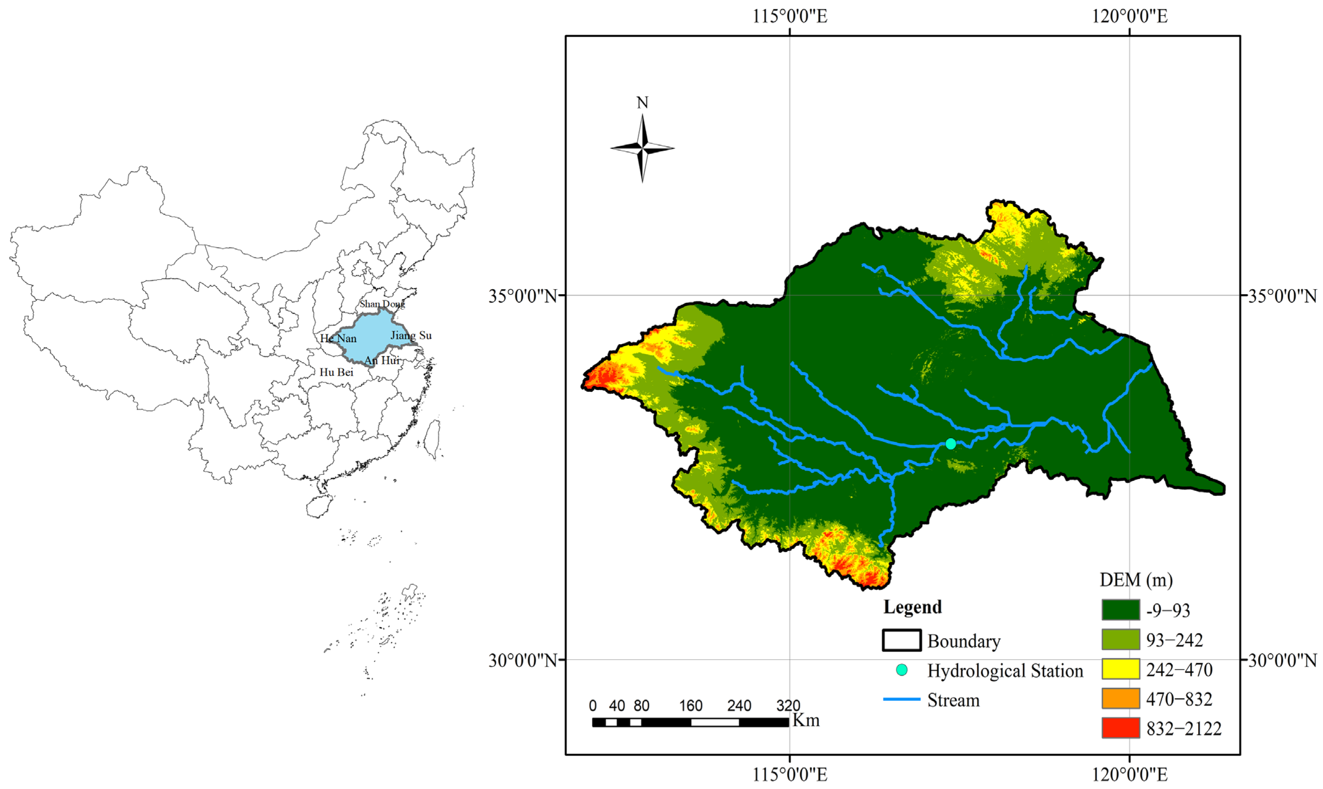
2.1. Study Area

The Huaihe River basin (HRB, Figure 1), located in the north–south climate transition zone, has an area of 270,000 km2. The north and the south parts of HRB belong to the warm temperate semi-humid monsoon and the subtropical humid monsoon climate zones, respectively. The elevation ranges from −9 m to 2122 m according to the SRTM 90 m digital elevation model (DEM) database (https://www.gscloud.cn/, accessed on 1 January 2020). The western, southwestern, and northeastern parts are mountainous and hilly areas, and the rest are vast plains. The Huai River originates from Tongbai Mountain in Henan province. It flows from west to east through Henan, Hubei, Anhui, and Jiangsu provinces. The total length and total drop of the river are approximately 1000 km and 200 m, respectively. The strata of HRB span two stratigraphic regions of North China and South China, and they are divided into three first-order tectonic units, namely the Sino-Korean quasi-platform, the Yangtze quasi-platform, and the Qinling fold area. The groundwater in HRB mainly consists of loose rock pore water, carbonate rock fissure karst water, and bedrock fissure water. In addition, loose rock pore water is the most widely distributed in the plain area. The lithology of water-bearing rock formations is mainly clayey soil, sand, and gravel, with a multi-layer structure.
The average annual rainfall is 878 mm, with large spatiotemporal differences. The average annual temperature ranges from 11 to 16 °C, increasing from the north to the south, from the coastal to the inland. The HRB is dry and rainless in winter and spring, and hot and rainy in autumn and summer. Thus, there is a sharp change between cold and warm, drought and flood. The average annual runoff depth is 230 mm. The discharge of upper reaches of Huaihe River is fast with high terrain and large river drop. However, the discharge is slow in the middle reach with low terrain and small river drop. In addition, the average annual evaporation of water surface is 900–1500 mm. The HRB has a large population, and it is an important grain production base in China. As a result, the water demand in the basin is large. However, drought disasters occur frequently in this basin, leading to an average of 2,698,000 hm2 of crops affected each year.

2.2. Data

For analyzing meteorological drought, hydrological drought, and agricultural drought, monthly precipitation (P), evapotranspiration (ET), potential evapotranspiration (PET), runoff (Q), soil moisture (SM), terrestrial water storage anomaly (TWS), and NDVI, were collected and averaged in HRB from 2002 to 2020. Particularly, monthly streamflow data at Bengbu hydrological station (Figure 1), a representative station of the main stream, was provided by the Huaihe River Commission of the Ministry of Water Resources. Other data were obtained from the following remote sensing data.

2.2.1. GPM_3IMERGM

The monthly precipitation was retrieved from the integrated multi-satellite retrievals for GPM (GPM_3IMERGM) with a spatial resolution of 0.1° × 0.1°. The temporal coverage was from June 2000 to October 2021. It was downloaded from https://disc.gsfc.nasa.gov/datasets/GPM_3IMERGM_06/summary?keywords=%22IMERG%20final%22, accessed on 22 November 2021.

2.2.2. MOD16A2

The ET and PET data were obtained from the Moderate-resolution Imaging Spectroradiometer (MODIS) Global Evapotranspiration Project MOD16A2 product. Their spatial and temporal resolutions were 500 m and 8 days, respectively. They were preprocessed by HDF-EOS to GeoTIFF (HEG) tool with extraction, projection, and spatial subset.

2.2.3. GLDAS_NOAH025_M 2.1

Soil moisture at depth of 0–10 cm (SM1), 10–40 cm (SM2), 40–100 cm (SM3), 100–200 cm (SM4); Snow depth water equivalent; and plant canopy surface water were provided by GLDAS Noah Land Surface Model L4 monthly 0.25 × 0.25 degree V2.1 (GLDAS_NOAH025_M 2.1).

2.2.4. GRACE/GRACE-FO Mascon

The monthly terrestrial water storage anomaly (TWS) used in this study was estimated by Center for Space Research (CSR) GRACE/GRACE-FO RL06 mass concentration (mascon) solutions (version 02). The Mascon solutions are the post-processing products based on spherical harmonic solutions, which are suitable for basin-scale (≥200,000 km2) analysis [48]. There was no need for any post-processing to obtain TWS information, which is convenient for non-geodesy and non-geophysics professionals [49]. The spatial resolution was 0.25° × 0.25°. Data beginning from April 2002 are available. The gap between data of GRACE and GRACE-FO mission, from July 2017 to May 2018, were reconstructed by linear regression using a dataset of reconstructed terrestrial water storage in China [50]. Other missing data were linearly interpolated [51,52,53].
The sources of TWS were assumed to be groundwater storage anomaly (GWS), surface water storage anomaly (SWS) including canopy water storage anomaly (CWS), soil moisture storage anomaly (SMS), and snow water equivalent anomaly. Thus, SWS and GWS can be determined as follows [54,55,56]:
SWS = CWS + SMS + SWE
GWS = TWS − SWS
where CMS, SWS, and SWE can be acquired from GLDAS Noah, and they were derived by subtraction of average values from 2004 to 2009 as TWS.

2.2.5. MOD13C2

The NDVI dataset was obtained from the MODIS Terra Vegetation Indices Monthly L3 Global 0.05Deg Climate Modeling Grid product (MOD13C2) [57], which was also preprocessed by HEG tool. Detailed information can be found at https://ladsweb.modaps.eosdis.nasa.gov/missions-and-measurements/products/MOD13C2, accessed on 18 March 2023.

3. Methods

3.1. Trend Analysis

The Mann–Kendall (M-K) test was used as a non-parametric test for assessing monotonous trends in hydrometeorology [58,59]. For time series xi (i = 1, 2,…, n), the statistic S can be calculated using:
S = i = 1 n j = i + 1 n 1 sgn x i x j
where sgn() is the sign function of (xixj). It equals 1, 0, −1, when (xixj) is greater than, equal, and less than 0, respectively.
The test statistic Z can be calculated as follows:
Z = S 1 VAR S ,   S > 0 0                       ,   S = 0 S + 1 VAR S ,   S < 0
where VAR(S) is the variance of S. The increasing or decreasing trend can be detected if Z is greater or smaller than 0, respectively. In addition, trends can be identified at the significance level of 0.10, 0.05, and 0.01, when the absolute value of Z is greater than 1.65, 1.96, and 2.58, respectively.
To estimate the trend magnitude of time series X further, the Kendall slope is defined [60]:
β = M e d i a n x i x j i j , 1 j < i n
where n is the length of X, and a positive/negative β value represents a rising/decreasing trend.

3.2. Drought Indicators

Various drought indicators were calculated, including standardized precipitation index (SPI), standardized evapotranspiration index (SEI), standardized precipitation evapotranspiration index (SPEI) for meteorological drought, standardized streamflow index (SSI) for hydrological drought, standardized soil moisture (SSMI), and standardized NDVI index (SNI) for agricultural drought. These indicators were used for analyzing the drought propagation further because they can be calculated for different accumulation times. In addition, the drought severity index (DSI) was used for assessing hydrological and agricultural drought.
SPI is a commonly used meteorological drought indicator [11]. The precipitation dataset was fitted by a theoretical probability distribution, for example, a Gamma distribution was used in this study. Then, the cumulative probability was converted to a standard normal distribution function. The level of drought was classified by the standardized cumulative frequency. SPI_n was calculated by the same procedure for different accumulation times n (ranging from 1 to 15 months in this study).
Following the same calculation procedure as SPI_n, SEI [61], SPEI [12], SSMI1–4 [62,63], SSI [64], and SNI [65] were derived for different accumulation times according to evapotranspiration, the difference between precipitation and potential evapotranspiration, SM1–4, streamflow, and NDVI, respectively.
The drought severity index (DSI) of TWS can be defined as its standardization as follows [17]:
DSI TWS i , j = TWS i , j TWS j σ j
where i and j are the year and month, respectively. TWSj represents the mean. σj is standard deviation. Drought levels can be classified as an exceptional drought (DSI ≤ −2.00), an extreme drought (−2.00 < DSI ≤ −1.60), a severe drought (−1.60 < DSI ≤ −1.30), a moderate drought (−0.79 < DSI ≤ −0.50), and no drought (DSI > −0.5).
Following the same procedure for the calculation of DSI-TWS, DSI-SM, DSI-Q, DSI-SWS, DSI-GWS [66], and DSI-NDVI [67] were also calculated for analyzing hydrological and agricultural drought further, according to SM, Q, SWS, GWS, and NDVI, respectively.

3.3. Correlation Analysis

The influencing factors of hydrological and agricultural drought were by cross-correlation coefficients among different variables at different times. The maximum cross-correlation coefficient between time series X(t) and Y(t + n) represents that Y is correlated most with X at lag time n, namely the response time can be assessed [68].
The drought propagation relationship was determined by Pearson correlation coefficients R between different drought indicators [25,27]. The correlation analysis between different types of drought was implemented as follows:
R i = corr ( X DSI TWS DSI SWS DSI GWS DSI Q DSI SM 1 DSI SM 2 DSI SM 3 DSI SM 4 DSI NDVI , Y SPI _ i SEI _ i SPEI _ i SSMI 1 _ i SSMI 2 _ i SSMI 3 _ i SSMI 4 _ i SSI _ i SNI _ i ) , 1 i 15
T = max ( R i ) scale , 1 i 15
where T indicates the propagation time i when the correlation coefficient Ri is the maximum value. In addition, the correlation coefficients between DSI-SM and SSMI, and between DSI-NDVI and SNI were not included here.

3.4. Machine Learning Methods for Drought Forecasting

3.4.1. Long Short-Term Memory Neural Network (LSTM)

The long short-term memory neural network (LSTM) is an improvement of traditional recurrent neural networks (RNN) introduced by Hochreiter and Schmidhuber [69]. The LSTM model consists of the recurrent LSTM memory cells, which are designed with input, forget, and output gates. The design can address the vanishing or exploding gradient problems during calculations of error back-propagation in traditional RNN [70]. Thus, it makes long-term temporal relationships between inputs and outputs easier to learn, and has been widely used in forecasting sequential data [71,72,73].

3.4.2. Convolutional Neural Network (CNN)

The convolutional neural network (CNN) is a modified version of feed-forward neural networks, which was developed by LeCun et al. [74]. Generally, the structure of CNN is composed of the convolution, pooling, and fully connected layers. The inputs of CNN are typically a two-dimensional matrix, such as images and sequence data with previous time steps. In the convolution layers, convolutional kernels with small size are used to encode information of inputs by tiled convolution. Pooling layers are down-sampled for extracting salient features from convolution layers by pooling filters. Finally, features obtained from the last pooling layer are flattened to feed to the fully connected layers. The processes of convolution and pooling improve the robustness of feature extraction and learning efficiency. Consequently, CNN has been successfully used for complex tasks in computer vision, natural language processing, and time series domains [75,76,77].

3.4.3. Categorical Boosting (CatBoost)

Categorical boosting (CatBoost), a machine learning library, was created by Russian search giant Yandex in 2017. CatBoost is an improved gradient-boosting decision tree algorithm (GBDT). In addition, it can handle classification and regression issues efficiently because of the following characteristics [78]. (1) Categorical features and numerical features can be trained together in the model by target statistics; (2) ordered boost is applied to reducing overfitting and prediction shift resulted from gradient bias; and (3) base predictors of CatBoost are oblivious trees with fewer parameters, which are balanced and less prone to overfitting. The superior performance, robustness, and fast prediction of CatBoost make it promising in hydrology [79,80].

3.5. Evaluation Criteria

The performances of drought forecasting models were evaluated by Nash–Sutclife efficiency (NSE) [81], root-mean-square error (RMSE), Pearson correlation coefficient (C), and threat score (TS) [82]:
NSE = 1 i = 1 n ( y i y ^ i ) 2 i = 1 n ( y i y ¯ ) 2
RMSE = 1 n i = 1 n ( y i y ^ i ) 2
C = i = 1 n ( y i y ¯ ) ( y ^ i y ^ ¯ ) i 1 n ( y i y ¯ ) 2 i 1 n ( y ^ i y ^ ¯ ) 2
TS = N h N h + N f + N m
where yi and y ^ i are the observed and forecasting values at time i, respectively; n is the length of observed or forecasting time series; and y ¯ and y ^ ¯ are the mean of the observations and forecasting values. Nh, Nf, and Nm are numbers of hits (both observations and forecasting values indicate the occurrence of drought), false alarms (forecasting values indicate drought but observations record no drought), and misses (observations record drought but forecasting values indicate no drought), respectively.
The ranges of NSE, C, and RMSE are ( , 1], [−1, +1], [0, + ), respectively. The NSE value becomes 1, when the forecasting values are exactly the same as the observed values. When predictions are worse than the simple average value, it becomes less than 0. Although it is sensitive to peak values, the values of NSE can effectively evaluate the degree of fit of the model [83]. The C value presents the linear correlation between predictions and observations. The value becomes 1, if they are a perfectly positive correlation. The RMSE values measure the deviations of the observed values from the predicted values, and its unit is consistent with the observations. The TS values range from 0 to 1, which can evaluate whether the model can correctly predict the occurrence of drought.

4. Results

4.1. Trend and Correlation Analysis of Different Variables

Figure 2 displays the trend analysis of P, ET, PET, SM1–4, Q, water storage anomaly, and NDVI values by the M-K test and Kendall slope methods. Increasing trends were found for the precipitation, evapotranspiration, potential evapotranspiration, and NDVI. In particular, the increasing trend of NDVI was significant at a confidence level of 95%. Although the precipitation increased, the water resource represented by soil moisture, runoff, and water storage in the Huaihe River basin decreased obviously. This may result from the evaporation loss, vegetation growth, and other human activities. Furthermore, the surface water storage, groundwater storage, and terrestrial water storage decreased significantly between June 2012, May 2015, and May 2013, respectively.
Figure 3 presents the maximum cross-correlation coefficients (R) among all variables at different lag time ranging from −15 to 15 months. Horizontal and vertical axes stand for the variable at time t and the variable at time t + n corresponding to the maximum coefficients, respectively. The response time can be indicated by the lag time of the maximum correlation coefficient. Generally, precipitation is a key factor affecting runoff and soil moisture. However, the relationships between precipitation and terrestrial water storage and groundwater storage were not obvious.
For runoff, the lag time between precipitation and runoff was 1 month with an R of 0.69. The runoff can affect SM4 with 1 month lag time with an R of 0.71. The changes of Q and SM1–2, ET, and TWS, were synchronized. For SM, the response time of both of SM1–2 to precipitation was 1 month. Synchronous changes were present among SM1–3. Compared with SM1–3, the changes of SM4 always lagged by 1 month.
In addition, water storage interacts with vegetation growth. All of the response times of NDVI to SM2–4 and SWS were 3 months, with negative correlation coefficients of −0.52, −0.52, −0.48, and −0.52, respectively. It shows the impact of plant uptake on water resources. The change of ET and NDVI were synchronous, and they were highly correlated with an R of 0.93.

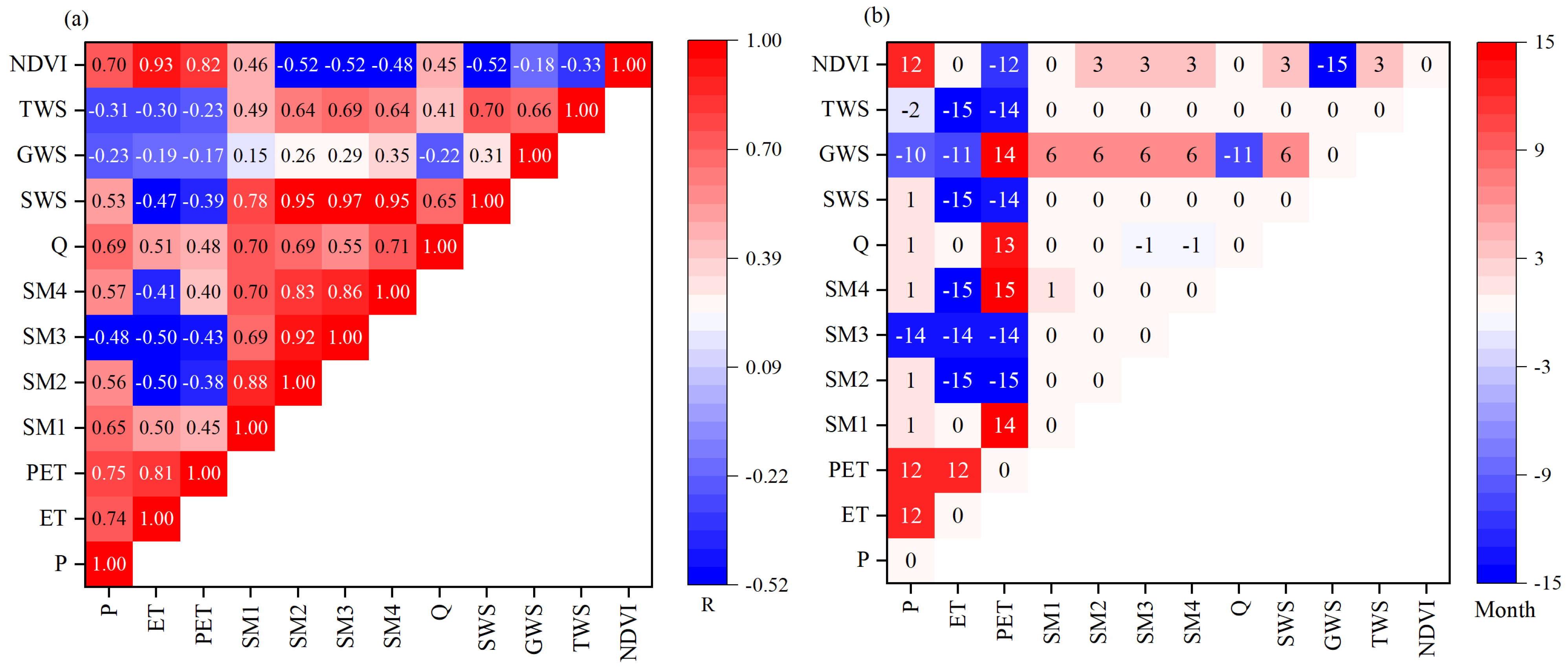
4.2. Correlation and Propagation time of Meteorological, Hydrological, and Agricultural Drought

Figure 4a,b represent the correlation and propagation times of meteorological, hydrological, and agricultural drought, respectively. The propagation time can be inferred from the maximum correlation coefficients between the DSI of different variables (described in the Y-axis), and SPI_n, SEI_n, SPEI_n, SSMI1/2/3/4_n, SSI_n, and SNI_n (described in the X-axis). For runoff drought, the relationship between DSI-Q and SPEI had the largest correlation coefficient with an R of 0.21. The propagation time from meteorological drought (SPEI) to hydrological drought (DSI-Q) may be 7 months. The soil drought was related to SPEI, SSI, and SPI. As the soil depth increases, the propagation time from meteorological and hydrological drought indicated by SPI, SEI, and SSI, to soil drought increases. SPEI had the greatest impact on soil drought with R of 0.60, 0.64, 0.67, and 0.67 for SM1–4, respectively. The propagation time from meteorological drought (SPEI) to soil drought at the depths of 0–10 cm, 10–40 cm, 40–100 cm, and 100–200 cm were about 3, 6, 8, and 11 months, respectively.
The correlation analysis of surface water storage drought was similar to soil drought, which was also affected by SPEI, SPI, and SSI. Compared with the correlation coefficients (greater than 0.60) between droughts of surface water storage and other types of drought (SPI, SPEI, SSMI, and SSI), the drought of groundwater storage had relatively low correlation coefficients with them (less than 0.44), indicating its complex influencing mechanism or the impacts of human activities [56,84]. Except for the soil drought indicators, which were directly related to the calculation of groundwater, only SEI_12 (R = 0.39) and SNI_12 (R = −0.31) were most relevant to the drought of groundwater storage.
In addition to SPEI and SPI, SNI was also related to the drought of terrestrial water storage. The impact of SNI on drought of terrestrial water storage was higher than the drought of soil, runoff, surface water storage, and groundwater storage. The propagation time from vegetation growth to the drought of terrestrial water storage may be 12 months. On the other hand, the soil moisture at depths of 100–200 cm affect the vegetation growth with an R of −0.36.

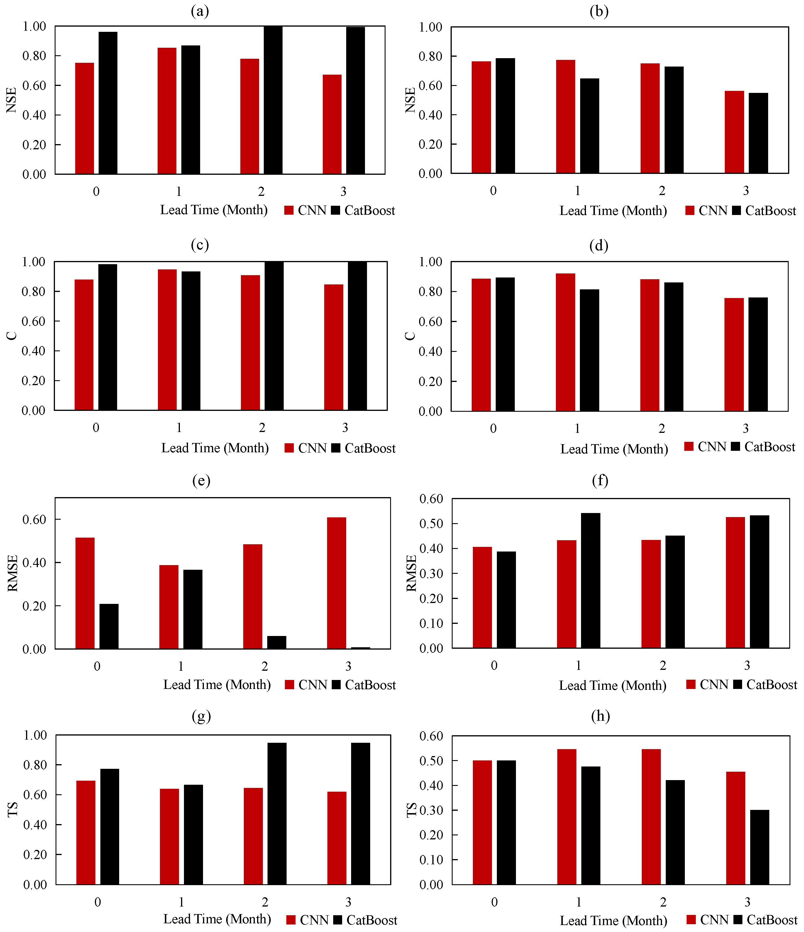
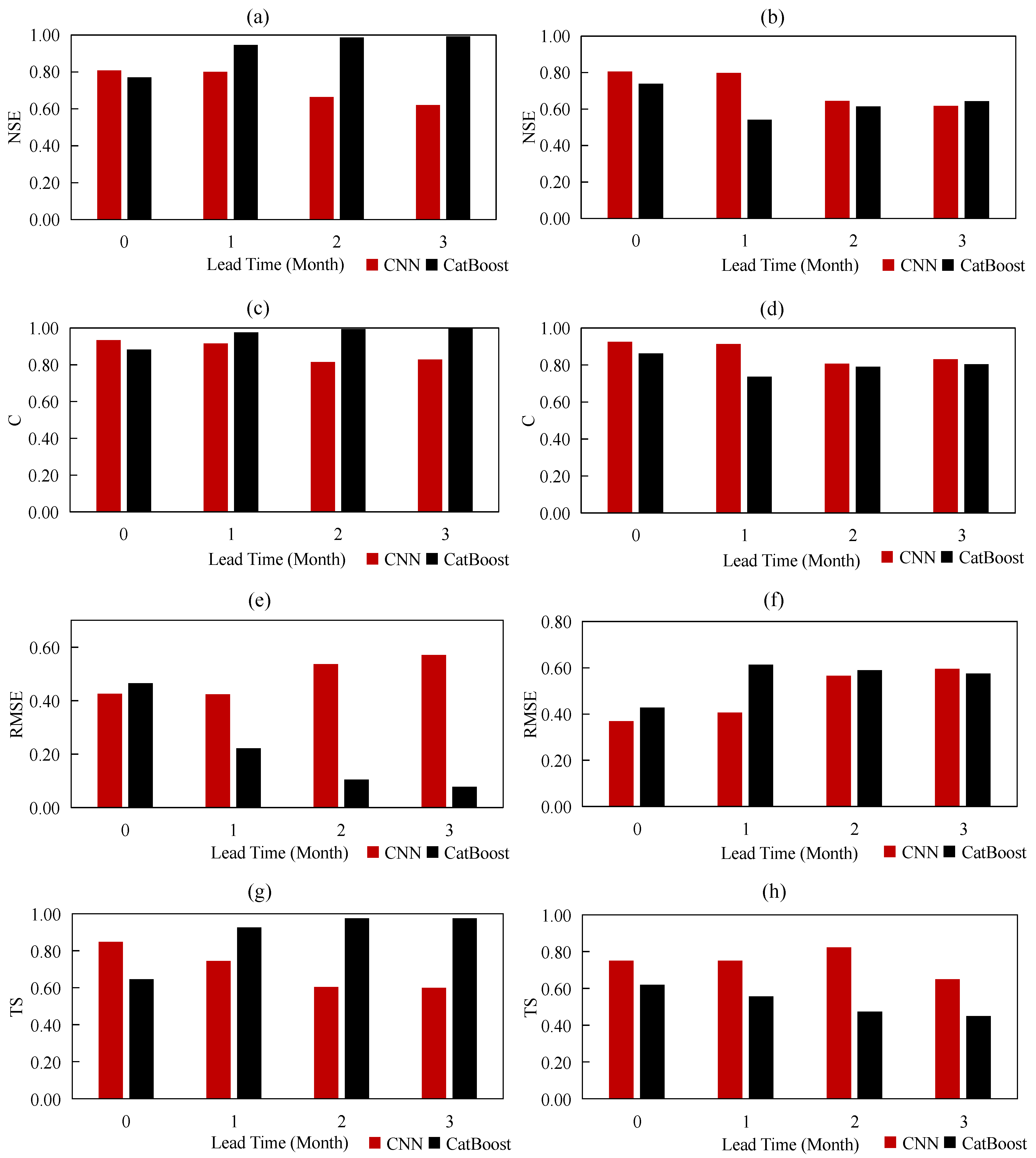
4.3. Performances of Drought Forecasting by LSTM, CNN, and CatBoost

According to the maximum Pearson correlation coefficients, predictors for hydrological drought and agricultural drought evaluated by DSI-TWS, DSI-GWS, and DSI-NDVI, were selected, which are shown in Table 1. These variables were normalized for constructing different machine learning methods at lead times n ranging from 0 to 3 months. The training and testing periods were 2002–2014, and 2015–2020, respectively.
The performances of terrestrial water storage drought forecasting by LSTM, CNN, and CatBoost models were assessed by NSE, C, RMSE, and TS (Table 2). With the extension of lead times, all of the models deteriorated for terrestrial water storage drought forecasting with NSE values ranging from 0.30 to 0.52, from 0.28 to 0.70, and from −0.66 to −0.13 for LSTM, CNN, and CatBoost during testing periods, respectively. The CNN model performed significantly better than LSTM and CatBoost in terms of NSE, C, and RMSE for lead times up to 2 months. For TS, the performance of LSTM was slightly better than that of CNN for lead times from 1 to 2 months. Despite the poor performance of LSTM and CNN for a three-month lead time, LSTM produced slightly higher NSE and C values, and lower RMSE value than CNN. That may have resulted from long-term dependencies of LSTM architecture for longer lead time forecasting. Regarding the CatBoost model, it was overfitting, which obtained excellent forecasting results during the training period and extremely poor performance with NSE less than 0 during the testing period.
The performances of models for groundwater and NDVI drought forecasting were worse than those for terrestrial water storage forecasting. That indicates more complicated influencing mechanisms for agricultural drought assessed by DSI-NDVI and groundwater drought than terrestrial water storage drought. The performances of LSTM and CNN for groundwater drought forecasting were similar, with NSE values at different lead times during testing periods ranging from 0.24 to 0.38, and from 0.25 to 0.33, respectively (Table 3 and Table 4). In addition, neither of them had the predictive ability for NDVI drought forecasting with NSE values less than 0 during testing periods. In addition, the CatBoost model was not shown because of its overfitting problem.

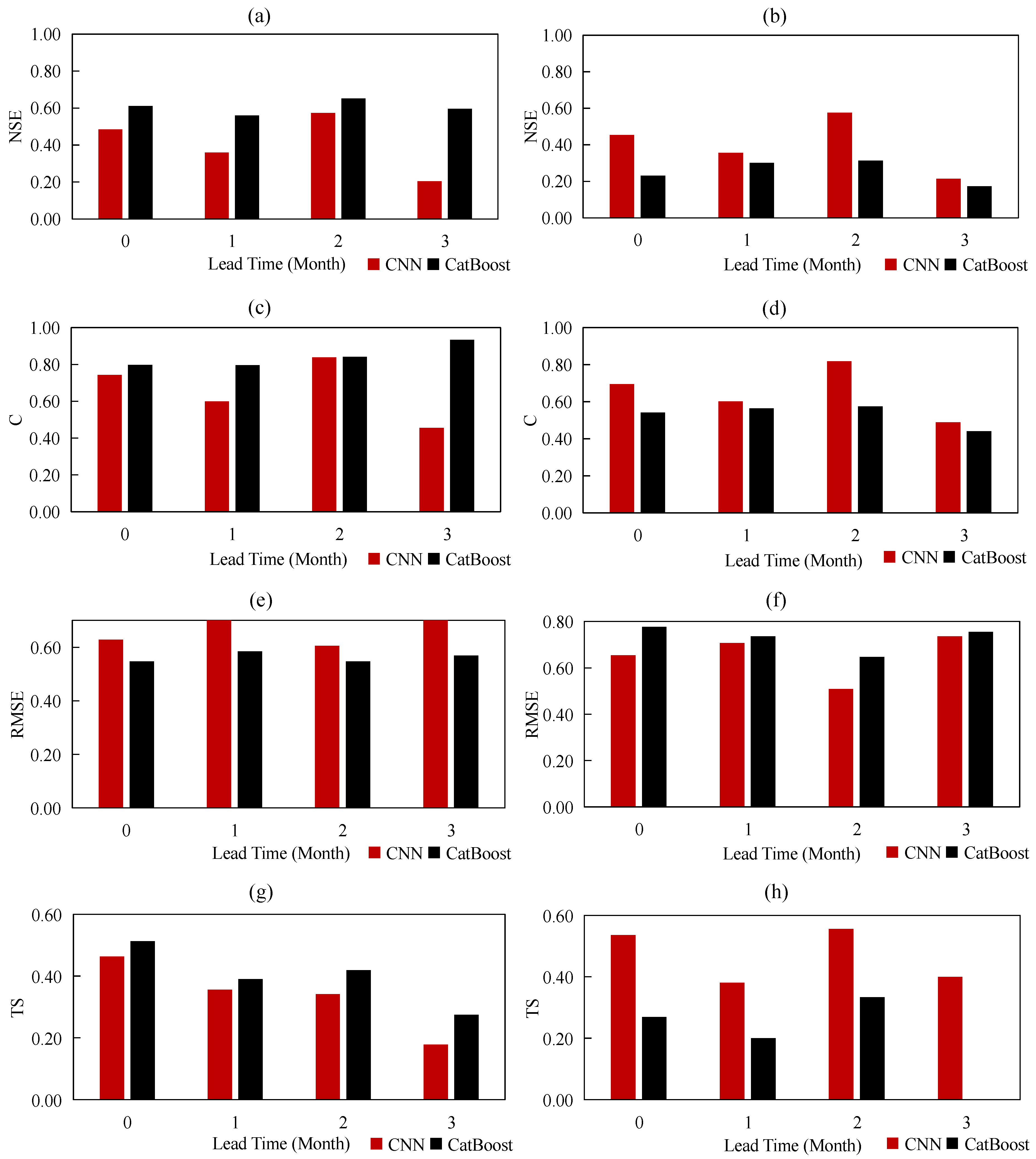
4.4. Performances of Drought Forecasting by CNN and CatBoost with Random Data Splitting for Training and Testing

Figure 5 presents the NSE, C, RMSE, and TS values of CNN and CatBoost models trained with random splitting datasets for terrestrial water storage drought forecasting at different lead times. The LSTM model was not shown here because only the sequential inputs were used for its recurrent architecture. To avoid the impact of data amount on models, the ratio of training data to testing data for random splitting was same as those divided in chronological order. With the random splitting for training and testing datasets, both of CNN and CatBoost models produced higher accuracy than those with training data divided in chronological order, respectively. Taking the performances at a 2-month lead time as an example, the improvements of NSE, C, RMSE, and TS values for CNN during testing were 103.45%, 27.09%, 35.32%, and 34.53%, respectively, and the improvements of NSE, C, RMSE, and TS values for CatBoost during testing were 230.03%, 24.93%, 57.31%, and 131.63%, respectively. This indicates the tendency may deteriorate the forecasting performances of CNN and CatBoost models. In other words, some of the trends’ influencing factors may be not selected as the model inputs; however, the random splitting for training and testing datasets eliminated the tendency as much as possible. Generally, the CNN model obtained better forecasting performances than the CatBoost model for terrestrial water storage drought forecasting.
The CatBoost produced satisfactory results for drought forecasting during testing periods compared with the trained with data divided in chronological order. This suggests the promise of the CatBoost model if the input–output relationship is stationary. Figure 6 illustrates the comparison of the CatBoost model trained with different datasets for terrestrial water storage drought forecasting at 1-month lead time as an example. The forecasting results for the CatBoost trained with data divided in chronological order matched with the observations perfectly during training periods. However, the model always overestimated during testing periods.
Figure 7 and Figure 8 illustrate the performances of CNN and CatBoost models trained with random data splitting for groundwater and agricultural drought forecasting, respectively. Similarly, both the CNN and CatBoost models with random data splitting for training and testing performed better. In addition, the CNN model always obtained higher accuracy than the CatBoost model. Taking the forecasting results at 1-month lead time as an example, Figure 9 presents the comparison of CNN models trained with different datasets. Although the forecasting results were unsatisfactory for extreme values, the trends of forecasting results were basically consistent with the observations. For the CatBoost models, the random splitting method also improved the model significantly. However, the obvious differences between performances during training and testing periods still existed.

5. Discussion

From the correlation analysis of raw variables and drought indicators, soil moisture (drought) always had a higher correlation than TWS (drought) with precipitation (SPI) and potential evapotranspiration (SPEI). This agrees with Forootan et al. [85] where the variations of soil moisture are dominated by precipitation, while terrestrial water storage involves complicated surface and subsurface processes. The significantly negative correlation coefficient between NDVI and deep soil moisture indicates the consumption of soil moisture for vegetation growth [86]. However, the controlling factors affecting terrestrial water storage and groundwater storage were unclear from the correlation analysis, which makes it difficult to reveal their mechanism [87,88].
The correlation relationships between various factors indicate droughts can be different with various drought indicators and calculation methods. Similarly, the propagation time from meteorological drought to hydrological and agricultural drought can vary with different approaches, such as correlation analysis by different correlation calculation methods. The uncertainties should be further assessed when they are used to unravel drought mechanisms.
In general, the drought of terrestrial water storage has higher correlations with other impact factors considered in this study than groundwater drought, followed by NDVI. Similarly, the forecasting performances of different machine learning methods were ranked by the drought of total terrestrial water storage, groundwater drought, and agricultural drought indicated by NDVI. It demonstrated better prediction of machine learning methods for stronger correlation between input and output. Kim et al. [89] discussed the better forecasting performances for streamflow forecasting in the high flow (higher autocorrelation coefficients) regime than those in the low flow regime. The data with no autocorrelation, deemed as white noise, is difficult to forecast [90].
The gridded remote sensing data used in this study were processed as an average for analyzing drought propagation and prediction in the HRB. Although temporal propagation from meteorological drought to hydrological and agricultural was analyzed by correlation analysis, the spatial characteristics of meteorological, hydrological, and agricultural droughts were not shown in this study. However, spatial-based assessment, including characteristics, propagation, and forecasting, is of great importance for the interpretation of drought mechanisms [91,92,93]. Thus, the integration of temporal and spatial characteristics and propagation will be the focus of future study. In addition, the drought evolution of onset, duration, extent, severity, and intensity should be analyzed further in different time scales and seasons.
According to the relatively low forecasting performances for hydrological and agricultural drought shown in Table 2, Table 3 and Table 4 some improvements need to be made, especially for the groundwater and NDVI drought forecasting. In addition, the change of groundwater storage derived from GRACE and GLDAS products was not validated. More data, such as the groundwater level, and hydrologeologic properties [47], the atmospheric circulation indices [94], spatiotemporal related variables, and human activities, etc., should be collected for comprehensive analysis of drought propagation and forecasting.
Although the impacts of other factors, such as the amount of training samples, on the prediction performances were controlled as much as possible, the uncertainty due to random splitting of training and testing data can still remain. Thus, the random splitting methods were utilized for the drought forecasting of terrestrial water storage, groundwater, and NDVI drought at lead times of 0–3 months to obtain more convincing results. For the comparison of different machine learning methods, the same training and testing data were used for drought forecasting after random splitting. However, all of the comparisons between machine learning methods trained with random splitting methods and those trained with data divided in chronological order indicated that the inconsistency between training and testing datasets resulted from the tendency can damage the generalization performances of machine learning models. Ovadia et al. [95] also discussed the predictive uncertainty under dataset shift between training data and testing data. In addition to the random splitting of training and testing data, more methods should be designed to deal with the nonstationary characteristics of the data [96,97].

6. Conclusions

The propagation from meteorological drought to hydrological drought and agricultural drought was analyzed based on correlation analysis in this study. However, the correlation analysis of original data and drought indicators are obviously different. For the correlation analysis of original data, precipitation is the key factor affecting soil water, runoff, and surfacewater storage with R values of 0.65, 0.69, and 0.53, respectively. Except for SM3, the changes of all of them responded to precipitation with a 1-month lag time. Evapotranspiration is also critical for the changes of soil water, runoff, and surfacewater storage. Except for shallow soil moisture at the depth of 0–10 cm, deep soil moisture was negatively correlated with evapotranspiration. It is worth noting the impacts of vegetation growth on consuming surface water storage and terrestrial water storage significantly with R values of −0.52 and −0.33, respectively. Thus, the interaction between vegetation growth and water resources should be explored further.
According to the correlation analysis of drought indicators, the propagation time from meteorological drought (SPEI) to runoff drought, surface water drought, and terrestrial water storage were around 7, 8, and 11 months with R values of 0.21, 0.68, and 0.48, respectively. In addition to the effects of meteorological drought on hydrological drought, the vegetation growth can lead to hydrological drought with 12-month a lag time. Furthermore, the agricultural drought indicated by vegetation growth can be also affected by the drought of soil moisture at depths ranging from 100 cm to 200 cm with an 8-month lag time, and an R value of −0.36.
For hydrological and agricultural drought forecasting, CNN always performed better than LSTM and CatBoost models, and different splitting methods of training and testing data showed a significant influence on the prediction of non-stationary data. The random data-splitting method improved the CNN and CatBoost models trained with data divided in chronological order obviously. For example, the maximum improvements of NSE, C, RMSE, and T values for terrestrial water storage drought forecasting based on CNN models were 103.45%, 27.09%, 35.32%, and 34.53%, respectively. While randomizing the training and test sets is a parsimonious approach for the improvement of non-stationary data forecasting, it is not suitable for recurrent models such as LSTM. New approaches should be introduced to explore the drought transmission mechanism under a changing environment.
The groundwater drought forecasting and agricultural drought forecasting indicated by NDVI were worse than the drought forecasting of terrestrial water storage even after the random splitting methods, suggesting the complicated influencing mechanisms of groundwater drought and vegetation growth. The data used were limited to the averaging time series in HRB. Data concerning variant spatiotemporal factors and invariant spatial properties should be integrated for a more comprehensive study of hydrological and agricultural drought mechanisms.

Author Contributions

Conceptualization, R.H. and H.Y.; Methodology, writing—original manuscript, and funding acquisition, R.H.; Visualization, H.Y.; Writing—review and editing, H.Y. and Y.-M.C. All authors have read and agreed to the published version of the manuscript.

Funding

Natural Science Research Project of Anhui Educational Committee (2022AH050832), the Academician Workstation in Anhui Province, Anhui University of Science and Technology (2022-AWAP-06), and Scientific Research Foundation for High-Level Talents of Anhui University of Science and Technology (13190207).

Data Availability Statement

All data used in this study can be accessed online. Precipitation from GPM can be downloaded from https://disc.gsfc.nasa.gov/datasets/GPM_3IMERGM_06/summary?keywords=%22IMERG%20final%22, accessed on 22 November 2021. Detailed information for evapotranspiration and potential evapotranspiration are available at https://ladsweb.modaps.eosdis.nasa.gov/missions-and-measurements/products/MOD16A2, accessed on 15 August 2021. Monthly streamflow can be accessed at http://www.hrc.gov.cn, accessed on 10 April 2023. GLDAS and GRACE data can be downloaded from https://disc.gsfc.nasa.gov/, accessed on 16 August 2021 and http://www2.csr.utexas.edu/grace/RL06_mascons.html, respectively. The NDVI dataset can be obtained from https://ladsweb.modaps.eosdis.nasa.gov/missions-and-measurements/products/MOD13C2, accessed on 18 March 2023.

Acknowledgments

All authors appreciate the organizations for providing public data used in this study. We thank the anonymous reviewers for their valuable suggestions.

Conflicts of Interest

The authors declare that they have no known competing financial interest or personal relationships that could have appeared to influence the work reported in this paper.

References

  1. Jones, R.L.; Guha-Sapir, D.; Ttubeuf, S. Human and economic impacts of natural disasters: Can we trust the global data? Sci. Data 2022, 9, 572. [Google Scholar] [CrossRef] [PubMed]
  2. Ma, F.; Yuan, X.; Ye, A. Seasonal drought predictability and forecast skill over China. J. Geophys. Res. Atmos. 2015, 120, 8264–8275. [Google Scholar] [CrossRef]
  3. Escobar, H. Drought triggers alarms in Brazil’s biggest metropolis. Science 2015, 347, 812. [Google Scholar] [CrossRef] [PubMed]
  4. Song, Y.; Park, M. Assessment of quantitative standards for mega-drought using data on drought damages. Sustainability 2020, 12, 3598. [Google Scholar] [CrossRef]
  5. Wilhite, D.A.; Glantz, M.H. Understanding the drought phenomenon: The role of definitions. Water Int. 1985, 10, 111–120. [Google Scholar] [CrossRef]
  6. American Meteorological Society (AMS). Statement on meteorological drought. Bull. Am. Meteorol. Soc. 2004, 85, 771–773. [Google Scholar] [CrossRef]
  7. Mishra, A.K.; Singh, V.P. A review of drought concepts. J. Hydrol. 2010, 391, 202–216. [Google Scholar] [CrossRef]
  8. Singh, C.; Jain, G.; Sukhwani, V.; Shaw, R. Losses and damages associated with slow-onset events: Urban drought and water insecurity in Asia. Curr. Opin. Environ. Sustain. 2021, 50, 72–86. [Google Scholar] [CrossRef]
  9. Crausbay, S.D.; Ramirez, A.R.; Carter, S.L.; Cross, M.S.; Hall, K.R.; Bathke, D.J.; Betancourt, J.L.; Colt, S.; Cravens, A.E.; Dalton, M.S. Defining ecological drought for the twenty-first century. Bull. Amer. Meteor. Soc. 2017, 98, 2543–2550. [Google Scholar] [CrossRef]
  10. Vicente-Serrano, S.M.; Quiring, S.M.; Peña-Gallardo, M.; Yuan, S.; Domínguez-Castro, F. A review of environmental droughts: Increased risk under global warming? Earth-Sci. Rev. 2020, 201, 102953. [Google Scholar] [CrossRef]
  11. McKee, T.B.; Doesken, N.J.; Kleist, J. The relationship of drought frequency and duration to time scales. Preprints. In Proceedings of the Eighth Conference on Applied Climatology, Anaheim, CA, USA, 17–22 January 1993; American Meteorological Society: Anaheim, CA, USA, 1993. [Google Scholar]
  12. Vicente-Serrano, S.M.; Begueria, S.; Lopez-Moreno, J.I. A multiscalar drought index sensitive to global warming: The Standardized Precipitation Evapotranspiration Index. J. Clim. 2010, 23, 1696–1718. [Google Scholar] [CrossRef]
  13. Shukla, S.; Wood, A.W. Use of a standardized runoff index for characterizing hydrologic drought. Geophys. Res. Lett. 2008, 35, L02405. [Google Scholar] [CrossRef]
  14. Mallick, K.; Bhattacharya, B.K.; Patel, N.K. Estimating volumetric surface moisture content for cropped soils using a Soil Wetness Index based on surface temperature and NDVI. Agric. For. Meteorol. 2009, 149, 1327–1342. [Google Scholar] [CrossRef]
  15. Marj, A.F.; Meijerink, A.M. Agricultural drought forecasting using satellite images, climate indices and artificial neural network. Int. J. Remote Sens. 2011, 32, 9707–9719. [Google Scholar] [CrossRef]
  16. Mu, Q.; Zhao, M.; Kimball, J.S.; McDowell, N.G.; Running, S.W. A remotely sensed global terrestrial Drought Severity Index. Bull. Am. Meteorol. Soc. 2013, 94, 83–98. [Google Scholar] [CrossRef]
  17. Zhao, M.; Geruo, A.; Velicogna, I.; Kimball, J.S. A global gridded dataset of GRACE Drought Severity Index for 2002–14: Comparison with PDSI and SPEI and a case study of the Australia millennium drought. J. Hydrometeorol. 2017, 18, 2117–2129. [Google Scholar] [CrossRef]
  18. Stefanidis, S.; Rossiou, D.; Proutsos, N. Drought Severity and Trends in a Mediterranean Oak Forest. Hydrology 2023, 10, 167. [Google Scholar] [CrossRef]
  19. Patil, R.; Polisgowdar, B.S.; Rathod, S.; Bandumula, N.; Mustac, I.; Reddy, G.V.S.; Wali, V.; Satishkumar, U.; Rao, S.; Kumar, A. Spatiotemporal characterization of drought magnitude, severity, and return period at various time scales in the Hyderabad Karnataka Region of India. Water 2023, 15, 2483. [Google Scholar] [CrossRef]
  20. Liu, S.; Chadwick, O.A.; Roberts, D.A.; Still, C.J. Relationships between GPP, satellite measures of greenness and canopy water content with soil moisture in mediterranean-climate grassland and oak savanna. Appl. Environ. Soil Sci. 2011, 2011, 839028. [Google Scholar] [CrossRef]
  21. Sang, L.; Zhu, G.; Xu, Y.; Sun, Z.; Zhang, Z.; Tong, H. Effects of agricultural large-and medium-sized reservoirs on hydrologic processes in the arid Shiyang River Basin, Northwest China. Water Resour. Res. 2023, 59, e2022WR033519. [Google Scholar] [CrossRef]
  22. Yin, L.; Wang, L.; Keim, B.D.; Konsoer, K.; Yin, Z.; Liu, M.; Zheng, W. Spatial and wavelet analysis of precipitation and river discharge during operation of the Three Gorges Dam, China. Ecol. Indic. 2023, 154, 110837. [Google Scholar] [CrossRef]
  23. Li, Y.; Mi, W.; Ji, L.; He, Q.; Yang, P.; Xie, S.; Bi, Y. Urbanization and agriculture intensification jointly enlarge the spatial inequality of river water quality. Sci. Total Environ. 2023, 878, 162559. [Google Scholar] [CrossRef] [PubMed]
  24. Wu, B.; Quan, Q.; Yang, S.; Dong, Y. A social-ecological coupling model for evaluating the human-water relationship in basins within the Budyko framework. J. Hydrol. 2023, 619, 129361. [Google Scholar] [CrossRef]
  25. Xu, Y.; Zhang, X.; Hao, Z.; Singh, V.P.; Hao, F. Characterization of agricultural drought propagation over China based on bivariate probabilistic quantification. J. Hydrol. 2021, 598, 126194. [Google Scholar] [CrossRef]
  26. Zhu, H.; Chen, K.; Hu, S.; Liu, J.; Shi, H.; Wei, G.; Chai, H.; Li, J.; Wang, T. Using the global navigation satellite system and precipitation data to establish the propagation characteristics of meteorological and hydrological drought in Yunnan, China. Water Resour. Res. 2023, 59, e2022WR033126. [Google Scholar] [CrossRef]
  27. Liu, Y.; Shan, F.; Yue, H.; Wang, X.; Fan, Y. Global analysis of the correlation and propagation among meteorological, agricultural, surface water, and groundwater droughts. J. Environ. Manag. 2023, 333, 117460. [Google Scholar] [CrossRef] [PubMed]
  28. Ho, S.; Tian, L.; Disse, M.; Tuo, Y. A new approach to quantify propagation time from meteorological to hydrological drought. J. Hydrol. 2021, 603, 127056. [Google Scholar] [CrossRef]
  29. Shi, H.; Zhao, Y.; Liu, S.; Cai, H.; Zhou, Z. A new perspective on drought propagation: Causality. Geophys. Res. Lett. 2022, 49, e2021GL096758. [Google Scholar] [CrossRef]
  30. Gao, C.; Liu, L.; Zhang, S.L.; Xu, Y.-P.; Wang, X.; Tang, X. Spatiotemporal patterns and propagation mechanism of meteorological droughts over Yangtze River Basin and Pearl River Basin based on complex network theory. Atmos. Res. 2023, 292, 106874. [Google Scholar] [CrossRef]
  31. Guo, Y.; Huang, S.; Huang, Q.; Leng, G.; Fang, W.; Wang, L.; Wang, H. Propagation thresholds of meteorological drought for triggering hydrological drought at various levels. Sci. Total Environ. 2020, 712, 136502. [Google Scholar] [CrossRef]
  32. Yu, M.; Liu, X.; Li, Q. Responses of meteorological drought-hydrological drought propagation to watershed scales in the upper Huaihe River basin, China. Environ. Sci. Pollut. Res. 2020, 27, 17561–17570. [Google Scholar] [CrossRef] [PubMed]
  33. Yang, F.; Duan, X.; Guo, Q.; Lu, S.; Hsu, K. The spatiotemporal variations and propagation of droughts in Plateau Mountains of China. Sci. Total Environ. 2022, 805, 150257. [Google Scholar] [CrossRef] [PubMed]
  34. Gong, R.; Chen, J.; Liang, Z.; Wu, C.; Tian, D.; Wu, J.; Li, S.; Zeng, G. Characterization and propagation from meteorological to groundwater drought in different aquifers with multiple timescales. J. Hydrol. Reg. Stud. 2023, 45, 101317. [Google Scholar] [CrossRef]
  35. Li, Z.; Huang, S.; Zhou, S.; Leng, G.; Liu, D.; Huang, Q.; Wang, H.; Han, Z.; Liang, H. Clarifying the propagation dynamics from meteorological to hydrological drought induced by climate change and direct human activities. J. Hydrometeorol. 2021, 22, 2359–2378. [Google Scholar] [CrossRef]
  36. Wang, J.; Wang, W.; Cheng, H.; Wang, H.; Zhu, Y. Propagation from meteorological to hydrological drought and its influencing factors in the Huaihe River Basin. Water 2021, 13, 1985. [Google Scholar] [CrossRef]
  37. Prodhan, F.A.; Zhang, J.; Hasan, S.S.; Sharma, T.P.T.; Mohana, H.P. A review of machine learning methods for drought hazard monitoring and forecasting: Current research trends, challenges, and future research directions. Environ. Modell. Softw. 2022, 149, 105327. [Google Scholar] [CrossRef]
  38. Hamitouche, M.; Molina, J. A review of ai methods for the prediction of high-flow extremal hydrology. Water Resour. Manag. 2022, 36, 3859–3876. [Google Scholar] [CrossRef]
  39. Dikshit, A.; Pradhan, B.; Alamri, A.M. Long lead time drought forecasting using lagged climate variables and a stacked long short-term memory model. Sci. Total Environ. 2021, 755, 142638. [Google Scholar] [CrossRef]
  40. Zhu, S.; Xu, Z.; Luo, X.; Liu, X.; Wang, R.; Zhang, M.; Huo, Z. Internal and external coupling of Gaussian mixture model and deep recurrent network for probabilistic drought forecasting. Int. J. Environ. Sci. Technol. 2021, 18, 1221–1236. [Google Scholar] [CrossRef]
  41. Adikari, K.E.; Shrestha, S.; Ratnayake, D.T.; Budhathoki, A.; Mohanasundaram, S.; Dailey, M.N. Evaluation of artificial intelligence models for flood and drought forecasting in arid and tropical regions. Environ. Modell. Softw. 2021, 144, 105136. [Google Scholar] [CrossRef]
  42. Wu, X.; Feng, X.; Wang, Z.; Chen, Y.; Deng, Z. Multi-source precipitation products assessment on drought monitoring across global major river basins. Atmos. Res. 2023, 295, 106982. [Google Scholar] [CrossRef]
  43. Tian, H.; Huang, N.; Niu, Z.; Qin, Y.; Pei, J.; Wang, J. Mapping winter crops in china with multi-source satellite imagery and phenology-based algorithm. Remote Sens. 2019, 11, 820. [Google Scholar] [CrossRef]
  44. Mohamed, A.; Faye, C.; Othman, A.; Abdelrady, A. Hydro-Geophysical evaluation of the regional variability of Senegal’s terrestrial water storage using time-variable gravity data. Remote Sens. 2022, 14, 4059. [Google Scholar] [CrossRef]
  45. Li, B.; Rodell, M.; Zaitchik, B.F.; Reichle, R.H.; Koster, R.D.; van Dam, T.M. Assimilation of GRACE terrestrial water storage into a land surface model: Evaluation and potential value for drought monitoring in western and central Europe. J. Hydrol. 2012, 446–447, 103–115. [Google Scholar] [CrossRef]
  46. Lopez, T.; Al Bitar, A.; Biancamaria, S.; Güntner, A.; Jaggi, A. On the use of satellite remote sensing to detect floods and droughts at large scales. Surv. Geophys. 2020, 41, 1461–1487. [Google Scholar] [CrossRef]
  47. Li, B.L.; Rodell, M.; Kumar, S.; Beaudoing, H.K.; Getirana, A.; Zaitchik, B.F.; de Goncalves, L.G.; Cossetin, C.; Bhanja, S.; Mukherjee, A.; et al. Global GRACE data assimilation for groundwater and drought monitoring: Advances and challenges. Water Resour. Res. 2019, 55, 7564–7586. [Google Scholar] [CrossRef]
  48. Zhang, L.; Sun, W.K. Progress and prospect of GRACE Mascon product and its application. Rev. Geophys. Planet. Phys. 2022, 53, 35–52. (In Chinese) [Google Scholar] [CrossRef]
  49. Save, H.; Bettadpur, S.; Tapley, B.D. High-resolution CSR GRACE RL05 mascons. J. Geophys. Res. Solid Earth 2016, 121, 7547–7569. [Google Scholar] [CrossRef]
  50. Zhong, Y.; Feng, W.; Zhong, M.; Ming, Z. Dataset of Reconstructed Terrestrial Water Storage in China Based on Precipitation (2002–2019); National Tibetan Plateau/Third Pole Environment Data Center: Beijing, China, 2020. [Google Scholar] [CrossRef]
  51. Long, D.; Yang, Y.; Wada, Y.; Hong, Y.; Liang, W.; Chen, Y.; Yong, B.; Hou, A.; Wei, J.; Chen, L. Deriving scaling factors using a global hydrological model to restore GRACE total water storage changes for China’s Yangtze River Basin. Remote Sens. Environ. 2015, 168, 177–193. [Google Scholar] [CrossRef]
  52. Yang, P.; Xia, J.; Zhan, C.; Qiao, Y.; Wang, Y. Monitoring the spatio-temporal changes of terrestrial water storage using GRACE data in the Tarim River basin between 2002 and 2015. Sci. Total Environ. 2017, 595, 218–228. [Google Scholar] [CrossRef]
  53. Sun, Z.; Zhu, X.; Pan, Y.; Zhang, J.; Liu, X. Drought evaluation using the GRACE terrestrial water storage deficit over the Yangtze River Basin, China. Sci. Total Environ. 2018, 634, 727–738. [Google Scholar] [CrossRef] [PubMed]
  54. Rodell, M.; Chen, J.; Kato, H.; Famiglietti, J.S.; Nigro, J.; Wilson, C.R. Estimating groundwater storage changes in the Mississippi River basin (USA) using GRACE. Hydrogeol. J. 2007, 15, 159–166. [Google Scholar] [CrossRef]
  55. Castle, S.L.; Thomas, B.F.; Reager, J.T.; Rodell, M.; Swenson, S.C.; Famiglietti, J.S. Groundwater depletion during drought threatens future water security of the Colorado River Basin. Geophys. Res. Lett. 2014, 41, 5904–5911. [Google Scholar] [CrossRef] [PubMed]
  56. Liu, M.; Pei, H.; Shen, Y. Evaluating dynamics of GRACE groundwater and its drought potential in Taihang Mountain Region, China. J. Hydrol. 2022, 612, 128156. [Google Scholar] [CrossRef]
  57. Didan, K. MOD13C2 MODIS/Terra Vegetation Indices Monthly L3 Global 0.05Deg CMG V006. 2015, Distributed by NASA EOSDIS Land Processes Distributed Active Archive Center. Available online: https://lpdaac.usgs.gov/products/mod13c2v006/ (accessed on 18 March 2023).
  58. Yue, S.; Pilon, P.; Cavadias, G. Power of the Mann-Kendall and Spearman’s rho tests for detecting monotonic trends in hydrological series. J. Hydrol. 2002, 259, 254–271. [Google Scholar] [CrossRef]
  59. Blahusiakova, A.; Matouskova, M. Rainfall and runoff regime trends in mountain catchments (Case study area: The upper Hron River basin, Slovakia). J. Hydrol. Hydromech. 2015, 63, 183–192. [Google Scholar] [CrossRef]
  60. Xu, Z.X.; Takeuchi, K.; Ishidaira, H. Long-term trends of annual temperature and precipitation time series in Japan. J. Hydrosci. Hydraul. Eng. 2002, 20, 11–26. [Google Scholar] [CrossRef]
  61. Das, P.K.; Midya, S.K.; Das, D.K.; Rao, G.S.; Raj, U. Characterizing Indian meteorological moisture anomaly condition using long-term (1901–2013) gridded data: A multivariate moisture anomaly index approach. Int. J. Climatol. 2018, 38, E144–E159. [Google Scholar] [CrossRef]
  62. Hao, Z.; AghaKouchak, A. Multivariate standardized drought index: A parametric multi-index model. Adv. Water Resour. 2013, 57, 12–18. [Google Scholar] [CrossRef]
  63. Zhang, H.; Ding, J.; Wang, Y.; Zhou, D.; Zhu, Q. Investigation about the correlation and propagation among meteorological, agricultural and groundwater droughts over humid and arid/semi-arid basins in China. J. Hydrol. 2021, 603, 127007. [Google Scholar] [CrossRef]
  64. Vicente-Serrano, S.M.; López-Moreno, J.I.; Beguería, S.; Lorenzo-Lacruz, J.; Azorín-Molina, C.; Morán-Tejeda, E. Accurate computation of a Streamflow Drought Index. J. Hydrol. Eng. 2012, 17, 318–332. [Google Scholar] [CrossRef]
  65. Nejadrekabi, M.; Eslamian, S.; Zareian, M.J. Spatial statistics techniques for SPEI and NDVI drought indices: A case study of Khuzestan Province. Int. J. Environ. Sci. Technol. 2022, 19, 6573–6594. [Google Scholar] [CrossRef] [PubMed]
  66. Han, Z.; Huang, S.; Huang, Q.; Leng, G.; Liu, Y.; Bai, Q.; He, P.; Liang, H.; Shi, W. GRACE-based high-resolution propagation threshold from meteorological to groundwater drought. Agric. For. Meteorol. 2021, 307, 108476. [Google Scholar] [CrossRef]
  67. Li, R.; Wang, J.; Zhao, T.; Shi, J. Index-based evaluation of vegetation response to meteorological drought in Northern China Normalized Difference Vegetation Index Anomaly (NDVIA). Nat. Hazards 2016, 84, 2179–2193. [Google Scholar] [CrossRef]
  68. Nygren, M.; Barthel, R.; Allen, D.M.; Giese, M. Exploring groundwater drought responsiveness in lowland post-glacial environments. Hydrogeol. J. 2022, 30, 1937–1961. [Google Scholar] [CrossRef]
  69. Hochreiter, S.; Schmidhuber, J. Long short-term memory. Neural Comput. 1997, 9, 1735–1780. [Google Scholar] [CrossRef] [PubMed]
  70. Hochreiter, S. The vanishing gradient problem during learning recurrent neural nets and problem solutions. Int. J. Uncertain. Fuzziness Knowl. Based Syst. 1998, 6, 107–116. [Google Scholar] [CrossRef]
  71. Anh, D.T.; Van, S.P.; Dang, T.D.; Hoang, L.P. Downscaling rainfall using deep learning long short-term memory and feedforward neural network. Int. J. Climatol. 2019, 39, 4170–4188. [Google Scholar] [CrossRef]
  72. Xiang, Z.; Jun, Y.; Demir, I. A rainfall-runoff model with LSTM-based sequence-to-sequence learning. Water Resour. Res. 2020, 56, e2019WR025326. [Google Scholar] [CrossRef]
  73. Hao, R.; Bai, Z. Comparative study for daily streamflow simulation with different machine learning methods. Water 2023, 15, 1179. [Google Scholar] [CrossRef]
  74. LeCun, Y.; Bottou, L.; Bengio, Y.; Haffner, P. Gradient-based learning applied to document recognition. Proc. IEEE 1998, 86, 2278–2324. [Google Scholar] [CrossRef]
  75. Simard, D.; Steinkraus, P.Y.; Platt, J.C. Best practices for convolutional neural networks applied to visual document analysis. In Proceedings of the Seventh International Conference on Document Analysis and Recognition, Edinburgh, UK, 6 August 2003; pp. 958–963. [Google Scholar]
  76. Taigman, Y.; Yang, M.; Ranzato, M.; Wolf, L. Deepface: Closing the gap to human-level performance in face verification. In Proceedings of the Conference on Computer Vision and Pattern Recognition, Columbus, OH, USA, 23–28 June 2014; pp. 1701–1708. [Google Scholar]
  77. Chen, C.; Hui, Q.; Xie, W.; Wan, S.; Zhou, Y.; Pei, Q. Convolutional Neural Networks for forecasting flood process in Internet-of-Things enabled smart city. Comput. Netw. 2021, 186, 107744. [Google Scholar] [CrossRef]
  78. Dorogush, A.V.; Ershov, V.; Gulin, A. CatBoost: Gradient boosting with categorical features support. arXiv 2018. [Google Scholar] [CrossRef]
  79. Huang, G.; Wu, L.; Ma, X.; Zhang, W.; Fan, J.; Yu, X.; Zeng, W.; Zhou, H. Evaluation of CatBoost method for prediction of reference evapotranspiration in humid regions. J. Hydrol. 2019, 574, 1029–1041. [Google Scholar] [CrossRef]
  80. Guo, Y.; Quan, L.; Song, L.; Liang, H. Construction of rapid early warning and comprehensive analysis models for urban waterlogging based on AutoML and comparison of the other three machine learning algorithms. J. Hydrol. 2022, 605, 127367. [Google Scholar] [CrossRef]
  81. Nash, J.E.; Sutcliffe, J.V. River flow forecasting through conceptual models, part 1: A discussion of principles. J. Hydrol. 1970, 10, 282–290. [Google Scholar] [CrossRef]
  82. Jollifee, I.T.; Stephenson, D.B. Forecast Verification: A Practitioner’s Guide in Atmospheric Science; John Wiley & Sons: Chichester, UK, 2003. [Google Scholar]
  83. Krause, P.; Boyle, D.P.; Fase, F. Comparison of different efficiency criteria for hydrological model assessment. Adv. Geosci. 2005, 5, 89–97. [Google Scholar] [CrossRef]
  84. Mustafa, S.M.T.; Abdollahi, K.; Verbeiren, B.; Huysmans, M. Identification of the influencing factors on groundwater drought and depletion in north-western Bangladesh. Hydrogeol. J. 2017, 25, 1357–1375. [Google Scholar] [CrossRef]
  85. Forootan, E.; Khaki, M.; Schumacher, M.; Wulfmeyer, V.; Mehrnegar, N.; van Dijk, A.I.J.M.; Brocca, L.; Farzaneh, S.; Akinluyi, F.; Ramillien, G.; et al. Understanding the global hydrological droughts of 2003–2016 and their relationships with teleconnections. Sci. Total Environ. 2019, 650, 2587–2604. [Google Scholar] [CrossRef]
  86. Yang, L.; Wei, W.; Chen, L.; Jia, F.; Mo, B. Spatial variations of shallow and deep soil moisture in the semi-arid Loess Plateau, China. Hydrol. Earth Syst. Sci. 2012, 16, 3199–3217. [Google Scholar] [CrossRef]
  87. Xie, X.; He, B.; Guo, L.; Miao, C.; Zhang, Y. Detecting hotspots of interactions between vegetation greenness and terrestrial water storage using satellite observations. Remote Sens. Environ. 2019, 231, 111259. [Google Scholar] [CrossRef]
  88. Wei, Z.; Wan, X. Spatial and temporal characteristics of NDVI in the Weihe River Basin and its correlation with terrestrial water storage. Remote Sens. 2022, 14, 5532. [Google Scholar] [CrossRef]
  89. Kim, T.; Yang, T.; Gao, S.; Zhang, L.; Ding, Z.; Wen, X.; Gourley, J.J.; Hong, Y. Can artificial intelligence and data-driven machine learning models match or even replace process-driven hydrologic models for streamflow simulation?: A case study of four watersheds with different hydro-climatic regions across the CONUS. J. Hydrol. 2021, 598, 126423. [Google Scholar] [CrossRef]
  90. Cruz-Nájera, M.A.; Treviño-Berrones, M.G.; Ponce-Flores, M.P.; Terán-Villanueva, J.D.; Castán-Rocha, J.A.; Ibarra-Martínez, S.; Santiago, A.; Laria-Menchaca, J. Short time series forecasting: Recommended methods and techniques. Symmetry 2022, 14, 1231. [Google Scholar] [CrossRef]
  91. Zhou, H.; Zhou, W.; Liu, Y.; Yuan, Y.; Huang, J.; Liu, Y. Identifying spatial extent of meteorological droughts: An examination over a humid region. J. Hydrol. 2020, 591, 125505. [Google Scholar] [CrossRef]
  92. Dikshit, A.; Dikshit, B.; Huete, A.; Park, H.-J. Spatial based drought assessment: Where are we heading? A review on the current status and future. Sci. Total Environ. 2022, 844, 157239. [Google Scholar] [CrossRef] [PubMed]
  93. Wang, T.; Tu, X.; Singh, V.P.; Chen, X.; Lin, K.; Zhou, Z. Drought prediction: Insights from the fusion of LSTM and multi-source factors. Sci. Total Environ. 2023, 902, 166361. [Google Scholar] [CrossRef]
  94. Bouguerra, H.; Derdous, O.; Tachi, S.E.; Hatzaki, M.; Abida, H. Spatiotemporal investigation of meteorological drought variability over northern Algeria and its relationship with different atmospheric circulation patterns. Theor. Appl. Climatol. 2023. [Google Scholar] [CrossRef]
  95. Ovadia, Y.; Fertig, E.; Ren, J.; Nado, Z.; Sculley, D.; Nowozin, S.; Dillon, J.V.; Lakshminarayanan, B.; Snoek, J. Can you trust your model’s uncertainty? Evaluating predictive uncertainty under dataset shift. In Proceedings of the 33rd International Conference on Neural Information Processing Systems, Vancouver, BC, Canada, 8–14 December 2019; pp. 14003–14014. [Google Scholar] [CrossRef]
  96. Kim, T.; Kim, J.; Tae, Y.; Park, C.; Choi, J.-H.; Choo, J. Reversible instance normalization for accurate time-series forecasting against distribution shift. In Proceedings of the ICLR 2022, Virtual Event, 25–29 April 2022. [Google Scholar]
  97. Liu, Y.; Wu, H.; Wang, J.; Long, M. Non-stationary Transformers: Exploring the stationarity in time series forecasting. arXiv 2022, arXiv:arXiv:2205.14415. [Google Scholar] [CrossRef]
Figure 1. Huaihe River basin.
Remotesensing 15 05524 g001
Figure 2. M-K test and Kendall slope of monthly time series.
Remotesensing 15 05524 g002
Figure 3. Pearson correlation analysis between different variables. (a) Correlation coefficients; (b) lag time.
Remotesensing 15 05524 g003
Figure 4. Pearson correlation analysis among meteorological drought, hydrological drought, and agricultural drought. (a) Maximum correlation coefficients; (b) propagation time. No significant correlations were shown in dotted line.
Remotesensing 15 05524 g004
Figure 5. Performances of CNN and CatBoost for terrestrial water storage drought forecasting during training (left column) and testing (right column) periods by random splitting at different lead times. (a,b) NSE; (c,d) C; (e,f) RMSE; (g,h) TS.
Remotesensing 15 05524 g005
Figure 6. Comparison of CatBoost models trained with different datasets for terrestrial water storage drought forecasting.
Remotesensing 15 05524 g006
Figure 7. Performances of CNN and CatBoost for groundwater drought forecasting during training (left column) and testing (right column) periods by random splitting at different lead times. (a,b) NSE; (c,d) C; (e,f) RMSE; (g,h) TS.
Remotesensing 15 05524 g007
Figure 8. Performances of CNN and CatBoost for agricultural drought forecasting during training (left column) and testing (right column) periods by random splitting at different lead times. (a,b) NSE; (c,d) C; (e,f) RMSE; (g,h) TS.
Remotesensing 15 05524 g008
Figure 9. Comparison of CNN models trained with different datasets for drought forecasting: (a) terrestrial water storage; (b) groundwater; (c) NDVI.
Remotesensing 15 05524 g009
Table 1. Inputs for drought forecasting models.
Forecasting VariablePredictors
DSI-TWS (t + n)SPI_12, SEI_12, SPEI_11, SSMI1_11, SSMI2_10, SSMI3_8, SSMI4_10, SSI_10, SNI-12, DSI-TWS (t − 1)
DSI-DWS (t + n)SPI_3, SEI_12, SNI-12, SSMI1_11, SSMI2_11, SSMI3_15, SSMI4_15, SSI_15, DSI-DWS (t − 1)
DSI-NDVI (t + n)SPI_2, SEI_13, SPEI_2, SSMI1_11, SSMI2_9, SSMI3_8, SSMI4_8, SSI_9, DSI-NDVI (t − 1)
Table 2. Comparison of terrestrial water storage drought forecasting with different models for lead times up to 3 months.
Model TypePeriodCriteriaTT + 1T + 2T + 3
LSTMTraining
(2000–2014)
NSE0.560.500.420.43
C0.760.710.660.66
RMSE0.560.600.650.64
TS0.540.440.440.35
Testing
(2015–2020)
NSE0.520.400.330.30
C0.770.710.630.65
RMSE0.580.650.690.70
TS0.390.510.450.42
CNNTraining
(2000–2014)
NSE0.730.540.370.27
C0.860.750.620.59
RMSE0.440.580.670.72
TS0.540.430.330.46
Testing
(2015–2020)
NSE0.700.550.370.28
C0.870.750.690.54
RMSE0.460.570.670.71
TS0.560.460.410.49
CatboostTraining
(2000–2014)
NSE0.950.990.980.92
C0.980.990.990.96
RMSE0.190.080.110.24
TS0.920.960.960.88
Testing
(2015–2020)
NSE−0.13−0.33−0.56−0.66
C0.820.780.690.31
RMSE0.890.971.061.09
TS0.390.390.180.09
Table 3. Comparison of LSTM and CNN for groundwater drought forecasting.
Model TypePeriodCriteriaTT + 1T + 2T + 3
LSTMTraining
(2000–2014)
NSE0.570.540.510.24
C0.770.730.720.50
RMSE0.440.460.470.58
TS0.430.360.220.00
Testing
(2015–2020)
NSE0.380.310.240.25
C0.700.670.720.68
RMSE0.730.780.820.81
TS0.520.540.350.58
CNNTraining
(2000–2014)
NSE0.320.480.280.35
C0.700.700.580.62
RMSE0.550.480.570.54
TS0.520.180.270.25
Testing
(2015–2020)
NSE0.330.320.260.33
C0.590.680.650.70
RMSE0.760.770.810.77
TS0.710.600.500.56
Table 4. Comparison of LSTM and CNN for agricultural drought forecasting.
Model TypePeriodCriteriaTT + 1T + 2T + 3
LSTMTraining
(2000–2014)
NSE0.280.09−0.03−0.24
C0.530.310.13−0.07
RMSE0.770.860.920.98
TS0.370.200.180.07
Testing
(2015–2020)
NSE−0.05−0.18−0.24−0.39
C0.150.20−0.170.06
RMSE0.740.780.790.84
TS0.000.000.000.00
CNNTraining
(2000–2014)
NSE−0.040.020.150.16
C0.230.300.400.41
RMSE0.920.890.830.81
TS0.210.260.360.30
Testing
(2015–2020)
NSE−0.10−0.22−0.32−0.40
C0.470.150.09−0.04
RMSE0.750.800.810.84
TS0.250.000.000.00
Disclaimer/Publisher’s Note: The statements, opinions and data contained in all publications are solely those of the individual author(s) and contributor(s) and not of MDPI and/or the editor(s). MDPI and/or the editor(s) disclaim responsibility for any injury to people or property resulting from any ideas, methods, instructions or products referred to in the content.

