A Cloud Water Path-Based Model for Cloudy-Sky Downward Longwave Radiation Estimation from FY-4A Data

Abstract

Clouds are a critical factor in regulating the climate system, and estimating cloudy-sky Surface Downward Longwave Radiation (SDLR) from satellite data is significant for global climate change research. The models based on cloud water path (CWP) are less affected by cloud parameter uncertainties and have superior accuracy in SDLR satellite estimation when compared to those empirical and parameterized models relying mainly on cloud fraction or cloud-base temperature. However, existing CWP-based models tend to overestimate the low SDLR values and underestimate the larger SDLR. This study found that this phenomenon was caused by the fact that the models do not account for the varying relationships between cloud radiative effects and key parameters under different Liquid Water Path (LWP) and Precipitable Water Vapor (PWV) ranges. Based upon this observation, this study utilized Fengyun-4A (FY-4A) cloud parameters and ERA5 data as data sources to develop a new CWP-based model where the model coefficients depend on the cloud phase and cloud water path range. The accuracy of the new model’s estimated SDLR is 20.8 W/m² for cloudy pixels, with accuracies of 19.4 W/m² and 23.5 W/m² for overcast and partly cloudy conditions, respectively. In contrast, the accuracy of the old CWP-based model was 22.4, 21.2, and 24.8 W/m², respectively. The underestimation and overestimation present in the old CWP-based model are effectively corrected by the new model. The new model exhibited higher accuracy under various station locations, cloud cover scenarios, and cloud phase conditions compared to the old one. Comparatively, the new model showcased its most remarkable improvements in situations involving overcast conditions, water clouds with low PWV and low LWP values, ice clouds with large PWV, and conditions with PWV ≥ 5 cm. Over a temporal scale, the new model effectively captured the seasonal variations in SDLR.

1. Introduction

Global climate change is a major challenge currently facing humanity. Downward Longwave Radiation at the Earth’s surface (SDLR) is an essential climate variable for the study of global climate evolution as defined by the Global Climate Observing System. Cloud covers more than 60% of the Earth’s surface and greatly affects the radiative balance of the earth–atmosphere system. Estimating cloud-sky SDLR data sets using satellite data is of great significance for radiative forcing and climate response research, energy balance research, and water cycle research. Currently, the spatial resolution and accuracy of satellite-estimated clear-sky SDLR have been greatly improved, with kilometer-scale instantaneous clear-sky SDLR accuracy ranging from 17 to 26 W/m² [1,2]. Conversely, there remains significant uncertainty in the accuracy of kilometer-scale instantaneous cloud-sky SDLR estimated by satellite, and the retrieval accuracy is much lower than that of clear-sky conditions [2,3,4,5].

Cloud-sky SDLR primarily originates from radiation emitted by clouds themselves and radiation contributions from the atmosphere below the cloud. When clouds are semi-transparent, SDLR also includes the portion of radiation above the clouds that penetrates the cloud layer and reaches the Earth’s surface. Given knowledge of the vertical characteristics of the atmosphere and clouds, SDLR can be accurately calculated by atmospheric radiative transfer models. Due to the extensive input parameters and complicated calculation processes required by radiative transfer models, SDLR estimation at high-resolution scales often relies on empirical models [3,6,7,8], parameterized models [4,9,10,11,12,13], and machine learning methods [14,15,16,17,18,19,20]. Although machine learning models offer the highest accuracy, empirical and parameterized models have clear analytical forms and interpretability, making them irreplaceable in satellite estimation.

In empirical and parameterized models, cloud radiative effects are described in four different forms. The first form is cloud fraction correction, which is used by most empirical models. These models describe clear-sky SDLR using surface air temperature and water vapor pressure, while cloud-sky SDLR is an empirical correction of clear-sky SDLR using a factor based on the cloud fraction [3,6,7,8]. Some researchers also used dew point temperature or cloud base height as correction factors [21,22]. Existing studies demonstrated that most empirical models rely on specific sites and datasets, requiring adjustments for use in other locations [23,24,25].

For the second form, cloud base temperature is used to represent cloud radiative effects because that cloud base temperature is a key parameter directly determining the radiation contribution of the cloud base [4,9,12,13,26,27]. However, since the information below clouds cannot be observed by optical sensors, the cloud base temperature and height inferred from optical satellite data have great uncertainties.

To avoid using cloud base parameters, some researchers utilize other cloud parameters to describe cloud radiative effects. For the third form, cloud water path (CWP) is used to describe cloud radiation. Since CWP is related to cloud height or cloud emissivity [10,12], researchers employed cloud liquid water path (LWP) and ice water path (IWP) as substitutes for cloud base height and determined the relationship between SDLR and CWP through statistical analysis [10,11]. The fourth method is based on the correlation between cloud-top temperature and cloud-base temperature, using cloud-top temperature to estimate cloudy-sky SDLR [15,16].

In our previous research, we evaluated the accuracy of the above types of models under different cloud parameter quality conditions [28]. We found that a model based on CWP proposed by [11], hereafter referred to as Zhou2007, was less impacted by the uncertainty of cloud parameters than other models. Under accurate cloud fraction and cloud base temperature conditions, the Zhou2007 model performed similarly to the best model based on cloud base temperature and much better than the model using cloud correction. For the satellite estimation with large cloud parameter errors, the accuracy of the other models exceeded 30 W/m², while the RMSE of the Zhou2007 model’s estimated cloudy SDLR remained below 25 W/m² [28]. When applying the Zhou2007 model to Fengyun-4A (FY4A) and GOES-16 data, the RMSE of cloudy-sky SDLR is 24.3 W/m² for FY-4A data and 21.3 W/m² for GOES-16 data [29]. Previous studies show that the Zhou2007 model tends to overestimate low cloudy-SDLR values and underestimate large cloudy-SDLR values [11,28,29]. Moreover, though the Zhou2007 model used LWP and IWP to describe cloudy SDLR, the radiative effects of different cloud phases are not separately considered.

In order to improve the accuracy of CWP-based models in satellite estimations of cloudy SDLR, this study will deeply analyze the problem of the Zhou2007 model and investigate the radiative effects of different cloud conditions. Based on this analysis, utilizing FY4A/AGRI cloud parameters and ERA5 as data sources, a new SDLR parameterized model considering the cloud phase and CWP range will be constructed and validated. Furthermore, the new model will be compared with the Zhou2007 model and calibrated Zhou2007 model after the coefficients are calibrated by this study’s data. This comparison will analyze the improvements in the new model in different cloud phases, different PWV ranges, and different cloud water paths relative to existing CWP-based models.

2. Data

The data employed in this study include satellite products, reanalysis data, and ground measurements, which are utilized to develop and validate the SDLR model.

Table 1. Satellite and reanalysis data used in SDLR estimation.

Sources	Products	Parameters	Resolution	Function
FY-4A	L1 GEO	Latitude, longitude	4 km	Geolocation
	CLM	Cloud mask	4 km	Cloud detection
	CFR	Cloud fraction	4 km	SDLR estimation
	CLP	Cloud phase	4 km
	CPD and CPN	Cloud liquid water path (LWP) and ice water path (IWP)	4 km
ERA5 reanalysis	ERA5 hourly data on pressure and single levels	2 m air temperature (Ta), PWV	0.25° hourly	SDLR estimation
USGS	GMTED2010	Surface elevation (DEM)	0.05°	Atmospheric profile interpolation

presents the detailed information on these datasets.

2.1. FY-4A Products

This study used the following FY-4A products from 2018 and 2019: (1) AGRI-L1 GEO data, which gives latitude and longitude; (2) Cloud Mask (CLM), Cloud Fraction Rate (CFR) and Cloud Phase (CLP) products, which offer the cloud mask, cloud fraction, and cloud phase [30,31]; and (3) Cloud Parameters for Daytime (CPD) and Cloud Parameters for Night-time (CPN), which offer the LWP and IWP parameters during daytime and night-time [31,32,33], respectively. The resolution of these FY-4A parameters is 4 km, once or twice each hour.

For the cases where cloud fraction information is missing, we employ cloud edge discrimination to determine cloud fraction based on the result of whether a pixel represents a cloud edge, according to [29]. If the pixel represents a cloud edge, we assign a cloud fraction value of 0.5; for pixels representing the cloud center, the cloud fraction is set to 1. When LWP information is missing for a water- or mixed-phase cloud pixel, we use a fill value of 300 g/m² for LWP, according to the method of [29]. Similarly, for a mixed or ice phase cloud pixel with missing IWP information, a fill value of 100 g/m² is applied to IWP.

2.2. ERA5 Reanalysis

We utilized the fifth-generation European Centre for Medium-Range Weather Forecasts reanalysis (ERA5) data to obtain atmospheric parameters. ERA5 is a comprehensive dataset that integrates climate model data with multiple observational sources using physical principles. It offers global estimates for various atmospheric, oceanic wave, and land surface parameters [34]. For our study, we selected the atmospheric temperature and humidity profiles on 37 pressure levels and atmospheric parameters at a single level, as outlined in Table 1 [35,36]. The original resolutions of these data are 0.25° and hourly.

The Ta and PWV corresponding to the resolution of cloudy pixels were obtained from the ERA5 data using the method proposed by [37]. First, the ERA5 data are downscaled to the spatiotemporal scale of satellite pixels through time and interpolations. Then, the atmospheric profiles above the Earth’s surface are extracted using GMTED2010 elevation data [38]. The Ta and PWV values are obtained from the final atmospheric profile.

2.3. Field Measurements

The field measurements corresponding to satellite data were collected from 32 sites of the Baseline Surface Radiation Network (BSRN) [39] and the National Tibetan Plateau Data Center (TPDC) [40,41,42,43,44]. Their locations are displayed in Figure 1, and their information is in Appendix A 

Table A1. Site information.

Label	Full Name	Latitude (Deg)	Longitude (Deg)	Elevation (m)	Land Cover	Temporal Resolution (min)
ASP a	Alice Springs	−23.798	133.888	547	Grassland	1
COC a	Cocos Island	−12.193	96.835	6	Grassland	1
DWN a	Darwin Met Office	−12.424	130.8925	32	Grassland	1
FUA a	Fukuoka	33.5817	130.375	3	Asphalt	1
GUR a	Gurgaon	28.4249	77.156	259	Shrub	1
HOW a	wrah	22.5535	88.3064	51	Shrub	1
ISH a	Ishigakijima	24.3367	124.1633	6	Asphalt	1
LYU a	Lanyu Island	22.037	121.5583	324	Mixed forest	1
MNM a	Minamitorishima	24.2883	153.9833	7	Grassland	1
SAP a	Sapporo	43.06	141.3283	17	Asphalt	1
TAT a	Tateno	36.05	140.1333	25	Grassland	1
TIR a	Tiruvallur	13.0923	79.9738	36	Rock	1
SDL b	Sidalong	38.428	99.926	3146	Forest	10
GUZ b	Guazhou	41.405	95.673	2014	Desert	10
MIG b	Mixed grassland super station	37.7032	98.5949	3718	Mixed grass	30
QH b	Qinghai Lake	36.5909	100.4999	3209	Water	10
DSL b	DaShaLong	38.8399	98.9406	3739	Wet meadow	10
AR b	Arou	38.0473	100.4643	3033	Grassland	10
JYL b	JingYangLing	37.8384	101.116	3750	Grassland	10
YK b	YaKou	38.0142	100.2421	4148	Grassland	10
DM b	DaMan	38.8555	100.3722	1556	Cropland	10
SDQ b	SiDaoQiao	42.0012	101.1374	873	Shrub	10
HEH b	HeiHe	38.827	100.4756	1560	Grassland	10
HZZ b	HuaZhaiZi	38.7659	100.3201	1731	Desert	10
HUM b	HuangMo	42.1135	100.9872	1054	Desert	10
MIF b	Mixed forest	41.9903	101.1335	874	Mixed shrub	10
ZY b	ZhangYe Wetland	38.9751	100.4464	1460	Wetland	10
DYK b	DaYeKou	38.556	100.286	2703	Grassland	10
DH b	Dunhuang WestLake	40.348	93.709	993	Wetland	10
LZ b	LinZe	39.238	100.062	1402	Cropland	10
LC b	LianCheng	36.692	102.737	2903	Forest	10
XYH b	XiYingHe	37.561	101.855	3616	Grassland	10

Note: The superscripts are defined as follows: ^a BSRN sites, ^b TPDC sites.

. Nine sites are located within the Qinghai–Tibet Plateau region: SDL, MIG, QH, DSL, AR, JYL, YK, LC, and XYH.

The meteorological and radiation parameters of these sites include surface air temperature and relative humidity, surface pressure, and upward longwave radiation. The measurements of BSRN and TPDC sites were averages of 1 and 10 min, respectively. The in situ SDLR corresponding to the satellite was interpolated from the two nearest records to the satellite transit time.

The longwave radiation was measured by Kipp & Zonen CNR1 Net Radiometers for TPDC sites and by Eppley precision infrared radiometers for BSRN sites. Though the wavelength ranges of these instruments are different, their reading has been calibrated to the total range of the entire longwave spectrum [46]. We employ the quality control methods provided by BSRN to remove measurements of SDLR that fall outside the physical limit, the extremely rare limit, and the inter-comparison limit [47]. The physical limit means the physical range of SDLR. The measurements beyond the extremely rare limit should be eliminated, if no physical reasons, such as extreme weather conditions, can be found. The inter-comparison limit is the range of SDLR based on other associated parameters. We used the limits values suitable for all latitudes and climate regimes in the BSRN Program. The physical limits for SDLR are 40–700 W/m², and the extremely rare limits are 60–500 W/m². The inter-comparison limit of SDLR in relation to air temperature and upward longwave radiation are as follows:

$$\begin{array}{l}0.4\times \sigma T_a^4<F_{all-sky}<\sigma T_a^4+25\\ SULR-300 {\mathrm{W}/\mathrm{m}}^2<F_{all-sky}<SULR+25 {\mathrm{W}/\mathrm{m}}^2\end{array}$$

where F_all-sky is all-sky SDLR, $SULR$ is upward longwave radiation, Ta is the 2 m air temperature, and σ is the Stefan–Boltzmann constant.

3. Methods

First, we utilized an atmosphere radiative transfer model for simulation to analyze the problems of the existing cloud water path-based model. In response to this problem, we developed a new cloud water path-based model and validated the new model using the testing data, as shown in Figure 2. Additionally, we calibrated the coefficients of existing cloud water path-based model using training dataset and compared them with our new model. Figure 2 illustrates the process of model construction and validation, where the overcast pixel data of 2018 were employed for model construction, and all data from 2018 and 2019 were used for model validation.

3.1. Problem Analysis of Zhou2007 Model

The Zhou2007 model proposed by [11] is the model used for CERES SDLR products. This model uses global satellite parameters and ground observations to establish statistical relationships between cloudy SDLR and PWV, upward longwave radiation, LWP, and IWP. For the Zhou2007 model, the cloudy SDLR (F_all-sky) is the sum of fluxes from cloudy and clear portions (F_overcast and F_clear), which is as follows:

$$F_{all-sky}=cf•F_{overcas\mathrm{t}}+(1-cf)•F_{clear}$$

(1)

where cf indicates cloud fraction. F_clear and F_overcast are as follows:

$$F_{clear}=37.687+0.474•SULR+94.190•\log (1+PWV)-4.935•\log (1+PWV)$$

(2)

$$\begin{array}{l}{F}_{overcast}=60.349+0.480•SULR+127.956•\log (1+PWV)-29.794•{[\log (1+PWV)]}^2\\ \hspace{1em}\hspace{1em}\hspace{1em}+1.626•\log (1+LWP)+0.535•\log (1+IWP)\end{array}$$

(3)

where $SULR=\sigma T_a^4$, σ is the Stefan–Boltzmann constant, Ta is the 2 m air temperature, PWV is in unit of cm, and LWP and IWP are in unit of g/m². The model coefficients were derived using CERES cloud parameters and ground-measured SDLR at 15 sites around the world.

Because LWP and IWP have a relatively small impact on SDLR in this model, the accuracy of retrieved SDLR is better than the parameterized models based on cloud base temperature and the empirical models based on cloud fraction correction when remote sensing cloud parameters have large uncertainties [26]. Previous studies have shown that the SDLR retrievals using this model for FY4A achieve an accuracy of 24.3 W/m², but there is an issue of overestimation in areas with low SDLR values [11,29]. In this study, to analyze the problems with the model, we used a test dataset to examine the relationship between SDLR errors and various input parameters. We found that large SDLR errors are related to PWV and LWP. Figure 3a indicates that there is significant uncertainty in SDLR when PWV is less than 2 cm, and positively biased samples seem much more than negative biased samples. Figure 3b shows significant errors in SDLR when LWP is less than 200 g/m². This may be related to the simplifications in the model itself, as the Zhou2007 model employs uniform model coefficients in all cases, and the consideration of cloud radiative contributions is very simple.

Previous studies have developed different relationships between SDLR and PWV [21,26]. To address the problem of large SDLR errors under low-PWV conditions, we intend to derive model coefficients under different PWV ranges, as previously used in existing research [21]. Concerning the problem of large SDLR errors in situations with low LWP, we utilized the moderate-resolution atmospheric transmission (MODTRAN) radiative transfer model to analyze the relationship between cloud SDLR and LWP. Then, the new model was constructed based on this analysis. As shown in Figure 4, we simulated the SDLR variation caused by LWP variation for the mid-summer atmosphere and five default cloud types in MODTRAN. We kept the atmospheric temperature and humidity profiles and other cloud and atmospheric parameters constant while varying the LWP. This allowed us to obtain cloud SDLR and cloud longwave radiative forcing data at different LWP values.

Figure 4a demonstrates that the relationship between SDLR and LWP varies with LWP. For LWP < 100 g/m², there is a clear positive logarithmic correlation between SDLR and LWP, but as LWP increases, the increment in SDLR becomes smaller. In contrast, the Zhou2007 model assumed a constant relationship between SDLR and LWP, leading to SDLR overestimation under low-LWP conditions and underestimation under high-LWP conditions. Furthermore, Figure 4b reveals that when LWP is below 50 g/m², the slope of cloud radiative forcing with respect to LWP is significantly greater than in other LWP ranges. When LWP exceeds 100 g/m², changes in LWP have little impact on cloud radiative forcing.

3.2. Constructing a CWP-Based Model Considering Cloud Phase and LWP Range

3.2.1. Model Principal

Based on the above analysis, we developed a new CWP-based model considering cloud phase and the range of LWP. In the new model, the cloudy SDLR is the same as Equation 1. To compare the difference in flux of cloudy portion between our model and the Zhou2007 model, the F_clear uses the same formula as Equation (2), and we only parameterize the flux in the cloudy sky portion.

For water- and mixed-phase cloud, besides being dependent on PWV and Ta, F_overcast is varied with LWP when LWP ≤ 100 g/m² and is not varied with LWP when LWP > 100 g/m²:

$$F_{overcast}=a_0+a_1•SULR+a_2•V+a_3•V^2+a_4•\log (1+LWP)$$

(4)

where $V=\sqrt{\mathrm{l}\mathrm{o}\mathrm{g}(1+PWV)}$, and this formulation is better than log(1 + PWV), as indicated in [38]. The coefficients a_i (i = 0,…, 4) are dependent on the range of LWP and PWV. When LWP > 100 g/m², a₄ = 0.

For ice cloud, overcast SDLR is determined by Ta, PWV, and IWP:

$$F_{overcast}=a_0+a_1•SULR+a_2•V+a_3•V^2+a_4•\log (1+IWP)$$

(5)

where the coefficients a_i (i = 0,…, 4) are dependent on the range of PWV.

3.2.2. Model Coefficient Derivation

We obtained model coefficients following the procedure shown in Figure 2. Firstly, we obtained quality-controlled PWV, Ta, LWP, IWP, cloud phase, and SDLR data from FY4A data, ERA5 data, and ground observation data. Then, we used the data from 2018 as our training dataset and the data from 2019 as our validation dataset. As shown in Figure 4, for liquid clouds, the relationship between LWP and cloudy SDLR is different for the three LWP ranges, which are less than 50 g/m², between 50 and 100 g/m², and greater than 100 g/m². Additionally, the relationship between cloudy SDLR and PWV is different for different PWV ranges, as suggested by [21]. Therefore, for liquid and mixed clouds, we performed separate coefficient regressions for these three LWP ranges, and within each LWP range, we considered PWV ≤ 2 cm and PWV > 2 cm separately. For ice clouds, because it was difficult to analyze the relationship between SDLR and IWP using MODTRAN radiative transfer models, we only obtained model coefficients for different water vapor conditions. Regression method was used in model derivation. Finally, our model considers eight different conditions, and their coefficients are presented in

Table 2. Coefficients of the new CPW-based parameterization for different cloud phase and LWP range.

Cloud Conditions	LWP Range (g/m2)	PWV (cm)	a0	a1	a2	a3	a4
Water and mixed phase cloud	(0, 50]	(0, 2]	32.9619	0.5469	70.3615	28.5630	−2.2896
		(2, 8)	−237.0998	0.7254	334.4421	−78.9135	6.4414
	(50, 100]	(0, 2]	−10.6017	0.5154	27.8440	73.3841	12.9042
		(2, 8)	9.6408	0.5733	15.1083	57.3603	8.3065
	(100, 4000)	(0, 2]	20.7546	0.3292	245.0102	−46.1900	—
		(2, 8)	123.5700	0.4503	−27.6544	75.0153	—
Ice cloud	0	(0, 2]	14.9959	0.3667	184.0043	−28.0156	6.2955
		(2, 8)	87.8222	0.4838	−21.7233	71.6096	3.4303

.

3.3. Calibrated-Zhou Model

To investigate whether the problem of the Zhou2007 model shown in Section 3.1 was due to not performing model coefficient calibration using local data, we calibrated the coefficients of overcast flux in the Zhou2007 model using our study’s training dataset. The new model using calibrated coefficients is referred to as the Calibrated-Zhou model. For the Calibrated-Zhou model, the clear-sky SDLR is same as Equation (2), and the overcast SDLR is as follows:

$$\begin{array}{l}{F}_{overcast}=88.1140+0.4011•SULR+110.1629•\log (1+PWV)-14.2779•{[\log (1+PWV)]}^2\\ \hspace{1em}\hspace{1em}\hspace{1em}+0.2867•\log (1+LWP)+0.9598•\log (1+IWP)\end{array}$$

(6)

where the parameters are the same as those in Equation (2). Both Zhou2007 and Calibrated-Zhou models are compared with our new CWP-based model.

4. Results

4.1. SDLR Retrievals of Training Dataset

Table 3. Results for different conditions in training dataset (overcast pixels of 2018). The root mean square error (RMSE) and mean bias error (MBE) are in W/m², R is correlation coefficient, and N is sample.

Cloud Conditions	LWP Range (g/m2)	PWV (cm)	N	Zhou2007			Calibrated-Zhou			New Model
				RMSE	MBE	R	RMSE	MBE	R	RMSE	MBE	R
Water and mixed- phase cloud	(0, 50]	(0, 2]	808	26.2	10.7	0.83	24.2	−0.5	0.82	23.8	−1.7	0.83
		(2, 8)	1517	18.2	−0.4	0.88	17.4	−1.9	0.85	15.0	0.0	0.88
		All	2325	21.3	3.4	0.94	20.0	−1.4	0.94	18.6	−0.6	0.95
	(50, 100]	(0, 2]	2414	23.3	8.3	0.91	22.4	−1.9	0.91	21.7	−0.6	0.91
		(2, 8)	2105	17.9	−1.5	0.88	16.9	−4.9	0.88	15.2	0.0	0.89
		ALL	4519	20.9	3.7	0.96	20.0	−3.3	0.96	19.0	−0.3	0.96
	(100, 4000)	(0, 2]	21,241	25.0	6.3	0.88	24.3	−4.1	0.88	23.3	−0.1	0.89
		(2, 8)	20,995	16.9	3.2	0.86	15.2	−1.1	0.88	15.0	0.0	0.88
		ALL	42,236	21.4	4.7	0.95	20.3	−2.6	0.95	19.6	0.0	0.95
Ice cloud	0	(0, 2]	12,281	21.7	−2.0	0.88	21.4	−4.4	0.88	20.3	−0.4	0.89
		(2, 8)	12,695	17.1	−5.9	0.90	13.7	2.3	0.92	13.1	0.0	0.92
		ALL	24,976	19.5	−4.0	0.95	17.9	−1.0	0.96	17.0	−0.2	0.96

presents the SDLR results calculated using the training dataset and different models. The new model shows improvements under various conditions. For water and mixed-phase clouds, the accuracies are 18.6, 19.0, and 19.6 W/m² for the three conditions of 0 g/m² < LWP ≤ 50 g/m², 50 g/m² < LWP ≤ 100 g/m², and LWP > 100 g/m², respectively. For ice clouds, the accuracies are 20.3 and 13.1 W/m² for PWV ≤ 2 and PWV > 2, respectively. Overall, the accuracy is lower when PWV ≤ 2 cm than when PWV > 2 cm. When PWV ≤ 2 cm, the RMSE of SDLR ranges from 20 to 23.8 W/m², whereas when PWV > 2, the RMSE ranges from 13.1 to 15.2 W/m². Compared to the existing Zhou2007 model, the new model shows an improvement of 1.7 to 4.1 W/m². The greatest improvement is observed under the condition of an ice cloud with PWV > 2 cm, where the RMSE decreases by 4.1 W/m². Though the Calibrated-Zhou model has higher accuracy than the Zhou2007 model due to coefficient calibration, its RMSE is still 0.2 to 2.2 W/m² larger than the new model.

Figure 5 displays the results of water and mixed-phase clouds and ice clouds. For the water and mixed-phase cloud pixels in the training dataset, the new model achieves an RMSE of 19.5 W/m², which is 1.8 W/m² smaller than that of the Zhou2007 model and 0.8 W/m² smaller than that of the Calibrated-Zhou model. Figure 5a–c indicate that, compared to the other two models, the new model exhibits better consistency with observations in the ranges of SDLR < 200 W/m² and SDLR > 400 W/m². For ice cloud pixels, the new model achieves an RMSE of 17.0 W/m², which represents a reduction of 2.5 W/m² and 0.9 W/m² in RMSE when compared to the Zhou2007 model and Calibrated-Zhou model, respectively. Figure 5d–f reveal that, for ice clouds, the most significant improvement with the new model is in the range of SDLR > 400 W/m².

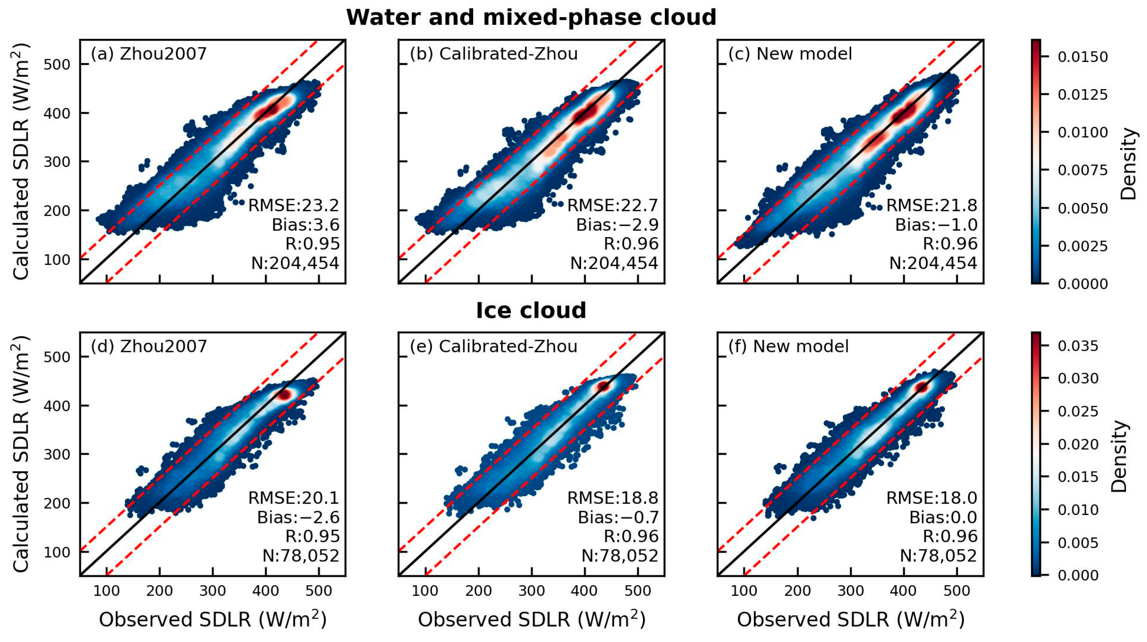
4.2. SDLR Retrievals of Testing Dataset

Figure 6 shows the results calculated using the testing dataset. For overcast pixels, the new model achieved an RMSE of 19.4 W/m², which is 1.8 W/m² smaller than that of the Zhou2007 model and 1.0 W/m² smaller than that of the Calibrated-Zhou model. For partly cloudy pixels, the new model achieved an RMSE of 19.4 W/m², which is 1.3 W/m² smaller than the Zhou2007 model and 0.7 W/m² smaller than the Calibrated-Zhou model. The improvement in retrieval accuracy under partly cloudy conditions is slightly less than that under overcast conditions. This is likely attributed to the fact that the new model was exclusively trained using overcast pixel data. For all the cloudy pixels, the new model achieved an RMSE of 20.8 W/m², which is 1.6 W/m² smaller than the Zhou2007 model and 0.9 W/m² smaller than the Calibrated-Zhou model. Furthermore, Figure 6 also illustrates that within the range of observed SDLR less than 200 W/m², both the Zhou2007 model and the Calibrated-Zhou model tend to overestimate, while the new model shows a significant improvement in this range. When the observed SDLR exceeds 400 W/m², the Zhou2007 model tends to underestimate SDLR, while SDLR from the new model exhibits better consistency with the observations.

Figure 7 displays the results for water and mixed-phase clouds and ice clouds based on the testing dataset. For water and mixed-phase clouds, the new model achieves an RMSE of 21.8 W/m², which is 1.4 W/m² smaller compared to the Zhou2007 model and 0.9 W/m² smaller compared to the Calibrated-Zhou model. It can be observed that the overestimation points of the Zhou2007 and the Calibrated-Zhou models in Figure 6, when SDLR is less than 200 W/m², occur under the conditions of water and mixed-phase clouds. For ice clouds, the new model achieves an RMSE of 18.0 W/m², which is 2.1 W/m² smaller compared to the Zhou2007 model and 0.8 W/m² smaller compared to the Calibrated-Zhou model. Similar to the results based on the training dataset (Figure 5), the existing models tend to underestimate in the high SDLR region, while the new model corrects this phenomenon.

Figure 8 presents the results at different sites. Overall, the accuracy of the Zhou2007 model is the lowest, followed by the Calibrated-Zhou model, while the new model yields the best results. For the new model, the RMSE ranges from 12.5 to 31.5 W/m², and the MBE ranges from −17.8 to 13.4 W/m². It performs best at the ISH station and worst at the YK station. The RMSEs of 27 sites are within 25 W/m². Sites with RMSEs exceeding 25 W/m² comprise DSL, JYL, YK, HZZ, and LC, with their corresponding MBE ± RMSE values as follows: 4.2 ± 27.4 W/m² (DSL), 0.6 ± 25.0 W/m² (JYL), −14.4 ± 31.5 W/m² (YK), 13.4 ± 25.7 W/m² (HZZ), and −4.5 ± 27.0 W/m² (LC). Compared to the Zhou2007 model, the new model improves accuracy at 31 sites, with improvements ranging from 0.01 to 5.9 W/m². The most significant improvement is observed at the HOW site. Compared to the Calibrated-Zhou model, the new model improves accuracy at 27 sites, with improvements ranging from 0.04 to 3.8 W/m², and the most significant improvement is observed at the YK site.

4.3. SDLR Results of Different Atmospheric and Cloud Conditions

To assess whether the new model has improved the retrieval accuracy under low-PWV and low-LWP conditions, we further analyzed the model’s results at different ranges of PWV and LWP.

Table 4. Same as Table 3, but for the results of all testing datasets.

Cloud Conditions	LWP Range (g/m2)	PWV (cm)	N	Zhou2007			Calibrated-Zhou			New Model
				RMSE	MBE	R	RMSE	MBE	R	RMSE	MBE	R
Water and mixed- phase cloud	(0, 50]	(0, 2]	5948	22.4	5.2	0.91	22.1	−2.7	0.91	21.2	−3.3	0.91
		(2, 8)	5735	17.5	−1.4	0.86	17.0	−3.4	0.86	15.8	−2.2	0.88
		All	11,683	20.1	1.9	0.95	19.8	−3.1	0.95	18.7	−2.7	0.96
	(50, 100]	(0, 2]	10,319	22.4	5.5	0.91	22.5	−3.6	0.91	21.6	−2.1	0.91
		(2, 8)	7133	17.4	−2.5	0.86	17.2	−6.0	0.87	15.8	−1.6	0.87
		ALL	17,452	20.5	2.2	0.96	20.5	−4.6	0.96	19.4	−1.9	0.96
	(100, 4000)	(0, 2]	106,999	26.5	6.4	0.90	26.0	−1.9	0.90	24.8	0.4	0.90
		(2, 8)	68,320	18.3	0.0	0.82	17.6	−4.1	0.84	17.3	−2.7	0.84
		ALL	175,319	23.7	3.9	0.95	23.1	−2.8	0.95	22.2	−0.8	0.96
Ice cloud	0	(0, 2]	45,033	21.8	−0.7	0.89	21.5	−3.1	0.89	20.6	0.0	0.90
		(2, 8)	33,019	17.4	−5.3	0.89	14.1	2.6	0.91	13.6	0.0	0.91
		ALL	78,052	20.1	−2.6	0.95	18.8	−0.7	0.96	18.0	0.0	0.96

presents the retrieval results from the test dataset under different conditions. For the new model, the retrieval accuracy for water and mixed-phase clouds in the LWP ranges of (0, 50), (50, 100), and (100, 4000) g/m² is 18.7, 19.4, and 22.2 W/m², respectively. The RMSE for ice clouds is 20.6 W/m² for PWV ≤ 2 cm and 13.6 W/m² for PWV > 2 cm. Similar to the results in Table 3, the results are better when PWV is higher compared to when it is lower. When PWV ≤ 2 cm, the RMSE is between 20.6 and 24.8 W/m², while for PWV > 2 cm, the RMSE ranges from 13.6 to 17.3 W/m². Compared to Table 3, the results based on the test dataset are similar to those based on the training dataset, but the accuracy is lower for LWP > 100 g/m². This is because the training dataset only includes overcast pixel data, whereas the test dataset includes overcast and partly cloudy pixel data. Compared to existing cloud water path-based models, the new model shows higher accuracy in each LWP and PWV range. Compared to the Zhou2007 model, the new model’s accuracy has increased by 0.8 to 3.8 W/m², with the largest improvement observed in higher-PWV conditions of ice cloud. Compared to the Calibrated-Zhou model, the new model’s accuracy has improved by 0.3 to 1.4 W/m².

Due to differences in retrieval accuracy for partly cloudy and overcast conditions, Figure 9 further analyzes the model accuracies within various PWV and CWP ranges for these two scenarios. Figure 9a,b illustrate that, for overcast pixels with different PWV and CWP values, the new model exhibits superior accuracy compared to the Zhou2007 model and the Calibrated-Zhou model. The most notable improvements are observed under the water and mixed-phase clouds with LWP ≤ 50 g/m² and ice clouds with larger PWV. Under overcast conditions with water and mixed-phase clouds and PWV ≤ 2 cm (conditions 1, 3, and 5), the Zhou2007 model shows an RMSE ranging from 23.4 to 25.3 W/m², with an MBE ranging from 5.9 to 11.2 W/m². Under these conditions, the Calibrated-Zhou model yields an MBE ranging from −0.8 to −4.3 W/m²; in comparison, the new model demonstrates an MBE ranging from −0.4 to −1.6 W/m², indicating a significant improvement in reducing SDLR overestimation under low-PWV conditions. For the ice clouds with PWV > 2 cm (condition 8), the Zhou2007 model shows an obvious negative bias, with an RMSE of 17.3 W/m² and an MBE of −5.8 W/m². The Calibrated-Zhou model reduces RMSE and MBE to 13.7 and 2.4 W/m², while the new model reduces the RMSE and MBE to 13.3 and −0.5 W/m². As shown in Figure 9c, for partly cloudy conditions, the new model demonstrates a noticeably improved accuracy compared to the Zhou2007 model under LWP ≤ 100 g/m² and PWV > 2 cm, LWP > 100 g/m² and PWV ≤ 2 cm, and ice clouds with PWV > 2 cm conditions (conditions 2, 4, 5, and 8), with RMSE decreasing in range from 1.15 to 1.97 W/m². Slight improvements are also observed under other conditions. On the contrary, the Calibrated-Zhou model shows larger errors for LWP ≤ 100 g/m² conditions. Figure 9d shows that, for partly cloudy pixels, the Zhou2007 model tends to overestimate under different cloud conditions when PWV ≤ 2 cm (conditions 1, 3, 5, and 7), while the new model rectifies this issue.

Figure 10 shows the box plot of SDLR errors from various models at different ranges of PWV. The corresponding values of the box plot are provided in the Supplementary Materials. The Interquartile Range (IQR) of SDLR errors, represented by the length of the boxes in the figure, is used to analyze the distribution of SDLR errors. It can be observed that when PWV ≤ 1 cm, the new model exhibits the greatest SDLR error (IQR = 35.9 W/m²). As PWV increases, SDLR errors show a decreasing trend, with an IQR of 8.7 W/m² when PWV > 7 cm. Compared to the Zhou2007 model, the new model shows significant improvements in different PWV regions, with both the IQR and median of SDLR errors decreasing. Within the PWV ≤ 3 cm range, the Zhou2007 model notably overestimates, while both the IQR and median of the new model decreased. Additionally, the Zhou2007 model exhibits a substantial underestimation when PWV > 5 cm, with an error median as large as −24.4 W/m², while the new model corrects it to be near 0. Although the Calibrated-Zhou model also shows improvements compared to the Zhou2007 model, its performance is noticeably inferior to the new model, particularly when 1 cm < PWV ≤ 2 cm, where this model exhibits a significant negative bias.

Figure 11 shows the variation in SDLR error from the model with LWP and IWP. Due to the scarcity of samples with LWP > 1000 g/m² and IWP > 1000 g/m², these samples were not included in the statistics. In Figure 11a, it can be observed that for each LWP range, the IQR of SDLR error from the new model is smaller than the other two models. The new model exhibits a minimum error comparable to the other two, while the maximum error is smaller. These findings indicate that the new model has a more concentrated error distribution within each range. At the same time, for LWP ≤ 100 g/m² and 250 g/m² < LWP ≤ 300 g/m², the Zhou2007 model overestimates significantly, while the SDLR error median of the new model is closer to 0, showing significant improvement within these LWP ranges. Figure 11b indicates that for various IWP ranges of ice clouds, both the IQR and median of SDLR error from the new model are better than those of the Zhou2007 model. The new model shows improvement in all IWP ranges. The new model corrects the increasing negative-bias trend with the increasing IWP that observed in the Zhou 2007 model.

Figure 11a,b also reveal that for water clouds and mixed clouds, the SDLR error is much larger, in the range of 250 g/m² < LWP ≤ 300 g/m², and a noticeable number of outliers are present. Concerning ice clouds, the most significant errors are found within the range of 0 g/m² < IWP ≤ 100 g/m². Upon analysis, this phenomenon is attributed to a substantial number of missing LWP and IWP values in satellite data, for which default values of 300 g/m² and 100 g/m² are assigned based on the cloud phase. In such cases, most SDLR errors fall within ±50 W/m², but a few have errors exceeding this range. In practical applications, the approach recommended in [10] can be employed, utilizing ERA5 cloud water paths to fill in missing values.

4.4. Seasonal Changes of Cloudy Skies SDLR

We further analyzed the agreement between the model estimations and observed values on a temporal scale. In this paper, data from nine sites located within the Qinghai–Tibet Plateau were used to analyze the seasonal variations of cloudy SDLR. Figure 12 presents the daily mean errors (E_daily) and daily mean values (F_daily) of the estimated SDLR from various models. The calculation formulas are as follows:

$$\begin{array}{c}{E}_{\mathrm{daily}}={\displaystyle \sum _{j=1}^N\left({\displaystyle \sum _{i=1}^M\left(F_{\mathrm{cacu},\mathrm{i},\mathrm{j}}-F_{\mathrm{obs},\mathrm{i},\mathrm{j}}\right)}\right)}/(M\ast N)\hfill \\ F_{\mathrm{daily}}={\displaystyle \sum _{j=1}^N\left({\displaystyle \sum _{i=1}^M{F}_{\mathrm{i},\mathrm{j}}}\right)}/(M\ast N)\hfill \end{array}$$

where j represents the site number, i represents a specific time of the day at that site, and $F_{\mathrm{cacu},\mathrm{i},\mathrm{j}}$ and $F_{\mathrm{obs},\mathrm{i},\mathrm{j}}$ represent the calculated and observed SDLR values for the corresponding site and time. N and M represent the total number of sites and the total number of valid times at the site. Figure 12a indicates that at the Qinghai–Tibet Plateau sites, the new model exhibits significant seasonal patterns in the average SDLR error. During the winter and early spring (Julian days 300 to 365 and 1 to 90), the errors show substantial fluctuations, ranging from −20 to 20 W/m², with some days having larger negative errors exceeding −20 W/m². In other seasons, the errors are smaller, with daily mean errors ranging from −15 to 10 W/m². In terms of the time scale, the new model has smaller errors compared to the other two models. Compared to the new model, the Zhou2007 model and the Calibrated-Zhou model exhibit substantial positive errors during the winter and early spring, while in other seasons, the Zhou2007 model has larger positive biases, and the Calibrated-Zhou model has larger negative biases. Figure 12b demonstrates that the new model captures the seasonal variations in SDLR effectively. Furthermore, the fluctuations in the SDLR of the new model are smaller than those of the observed values. The new model tends to overestimate the lower SDLRs during the winter and early spring, while it underestimates the relatively higher SDLRs between Julian days 50 and 300.

5. Discussion

Compared to other types of parameterized models, the CWP-based models are less affected by cloud parameter uncertainties and exhibit higher accuracy in satellite estimations. The existing optimal CWP-based model, the Zhou2007 model, has problems with overestimating low SDLR values and underestimating SDLR values. This study identified that these problems arise because the Zhou2007 model does not account for the varying relationships between cloud radiative effects and key parameters across different ranges of LWP and PWV. Based on this finding, this study developed a new CWP-based model, which shows the following advantages compared to the old CWP-based model.

Firstly, the new model has higher accuracy overall. Compared to the Zhou2007 model, the new model’s accuracy improved by 1.8 W/m2 for overcast conditions and by 1.3 W/m2 for partly cloudy conditions, respectively. The new model improved accuracy by 1.4 W/m² for water and mixed-phase clouds and by 2.1 W/m² for ice clouds, respectively.

Then, the new model performs better than the Zhou2007 model under almost all atmospheric and cloud conditions. The most significant improvements are observed in overcast conditions, low-PWV and low-LWP conditions for water and mixed-phase clouds, high-PWV conditions for ice clouds, and conditions with PWV ≥ 5 cm. Under overcast conditions, the Zhou 2007 model overestimated the SDLR by 5.9 to 11.2 W/m² for water and mixed-phase clouds with PWV ≤ 2 cm, while the new model reduced the MBE from −0.7 to −1.6 W/m² (Figure 9a, b). For ice clouds with PWV > 2 cm, the Zhou 2007 model showed a notable negative bias, with an MBE of −5.8 W/m², and the new model reduced it to −0.5 W/m² (Figure 9a, b). Figure 10 indicates that the Zhou 2007 model overestimates significantly in PWV ranges (0, 1], (1, 2], and (2, 3] cm, but substantially underestimates for PWV ≥ 5 cm (with a median error as high as −24.4 W/m²), while the new model exhibits significantly reduced SDLR errors. In the LWP ranges of (0, 50], (50, 100], and (250, 300] g/m², the new model notably rectified the Zhou 2007 model’s overestimation. For ice clouds, the new model corrects the trend of error increase with IWP that was present in the Zhou 2007 model.

Furthermore, to exclude the influence of the training dataset on model accuracy, we also calibrated the coefficients of the Zhou2007 model using our training dataset. While the Calibrated-Zhou model improved the accuracy of SDLR estimation relative to the Zhou2007 model, the phenomenon of overestimation of the small-SDLR values and underestimation of the large values still persisted, and its accuracy remained inferior to our new model.

The new model still has some limitations, which can be improved in the following aspects: (1) The SDLR error for PWV ≤ 1 cm is notably larger than for other PWV conditions, as shown in Figure 10. We found that even performing separate coefficient fitting for this region alone cannot resolve this issue. In future studies, exploring new model forms specifically for PWV ≤ 1 cm is necessary. (2) SDLR accuracy in partly cloudy conditions is worse than in overcast situations, possibly due to inaccuracies in estimating clear-sky flux in cloudy pixels or significant errors in cloud fraction for partly cloudy scenes. This study only models overcast conditions, and the clear portion flux of partly cloudy SDLR still adopts the Zhou2007 model. In future studies, the SDLR accuracy of partly cloudy conditions can be improved by employing more accurate clear-sky SDLR models or by modeling partly cloudy scenarios separately. (3) Because of MODTRAN’s limited flexibility in defining ice cloud properties, this study did not theoretically analyze the impact of IWP variations on the SDLR. In future studies, more advanced radiative transfer models can be used in ice cloud analysis and subsequently develop parameterized SDLR models for ice clouds.

6. Conclusions

The CWP-based model can serve as a practical parameterized model for satellite estimation of cloudy SDLR. This study developed a new CWP-based model that expresses overcast SDLR by PWV, Ta, LWP, and IWP, with model coefficients dependent on cloud phase, CWP, and PWV ranges, using FY4A/AGRI cloud parameters and ERA5 data as data sources.

The new model exhibits good performance in cloudy SDLR estimation. The accuracy of the cloudy SDLR estimated by the new model is 20.8 W/m², with accuracies of 19.4 W/m² and 23.5 W/m² for overcast and partly cloudy conditions, respectively. The accuracy of the new model is 21.8 W/m² for water and mixed-phase clouds and 18.0 W/m² for ice clouds. In detail, results when PWV >2 cm are better than those when PWV≤ 2 cm; results when LWP ≤ 100 g/m² are better than those when LWP > 100 g/m².

Compared to the old CWP-based model, the new model accounts for the varying relationships between cloud radiative effects and key parameters across different ranges of LWP and PWV, therefore effectively correcting the overestimation at smaller SDLR values and underestimation at larger values produced by the Zhou2007 model. The new model also shows improvements in different cloud cover scenarios, different cloud phase conditions, and different PWV and CWP ranges.

Overall, by considering the model coefficients’ dependence on LWP and PWV ranges and cloud phase, the proposed model has improved the cloudy SDLR accuracy of CWP-based models. The new model provides an effective means for satellite estimation of cloudy SDLR. Although this model is based on FY-4A data, it can be extended to MODIS, GOES-16, and other satellites in the future through model coefficient calibration.

References

1. Kratz, D.P.; Gupta, S.K.; Wilber, A.C.; Sothcott, V.E. Validation of the CERES Edition 2B Surface-Only Flux Algorithms. J. Appl. Meteorol. Climatol. 2010, 49, 164–180. [Google Scholar] [CrossRef]
2. Zeng, Q.; Cheng, J.; Dong, L. Assessment of the Long-Term High-Spatial-Resolution Global LAnd Surface Satellite (GLASS) Surface Longwave Radiation Product Using Ground Measurements. IEEE J. Sel. Top. Appl. Earth Obs. Remote Sens. 2020, 13, 2032–2055. [Google Scholar] [CrossRef]
3. Bisht, G.; Bras, R.L. Estimation of net radiation from the MODIS data under all sky conditions: Southern Great Plains case study. Remote Sens. Environ. 2010, 114, 1522–1534. [Google Scholar] [CrossRef]
4. Wang, T.; Shi, J.; Yu, Y.; Husi, L.; Ling, C. Cloudy-sky land surface longwave downward radiation (LWDR) estimation by integrating MODIS and AIRS/AMSU measurements. Remote Sens. Environ. 2018, 205, 100–111. [Google Scholar] [CrossRef]
5. Jiang, Y.; Tang, B.-H.; Zhang, H. Estimation of downwelling surface longwave radiation for cloudy skies by considering the radiation effect from the entire cloud layers. Remote Sens. Environ. 2023, 298, 113829. [Google Scholar] [CrossRef]
6. Crawford, T.M.; Duchon, C.E. An Improved Parameterization for Estimating Effective Atmospheric Emissivity for Use in Calculating Daytime Downwelling Longwave Radiation. Appl. Meteorol. Climatol. 1999, 38, 474–480. [Google Scholar] [CrossRef]
7. Iziomon, M.G.; Mayer, H.; Matzarakis, A. Downward atmospheric longwave irradiance under clear and cloudy skies: Measurement and parameterization. J. Atmos. Sol.-Terr. Phys. 2003, 65, 1107–1116. [Google Scholar] [CrossRef]
8. Li, M.Y.; Jiang, Y.J.; Coimbra, C.F.M. On the determination of atmospheric longwave irradiance under all-sky conditions. Sol. Energy 2017, 144, 40–48. [Google Scholar] [CrossRef]
9. Schmetz, P.; Schmetz, J.; Raschke, E. Estimation of daytime downward longwave radiation at the surface from satellite and grid point data. Theor. Appl. Climatol. 1986, 37, 136–149. [Google Scholar] [CrossRef]
10. Zhou, Y.P.; Cess, R.D. Algorithm development strategies for retrieving the downwelling longwave flux at the Earth’s surface. J. Geophys. Res. Atmos. 2001, 106, 12477–12488. [Google Scholar] [CrossRef]
11. Zhou, Y.P.; Kratz, D.P.; Wilber, A.C.; Gupta, S.K.; Cess, R.D. An improved algorithm for retrieving surface downwelling longwave radiation from satellite measurements. J. Geophys. Res. Atmos. 2007, 112, D15102. [Google Scholar] [CrossRef]
12. Forman, B.A.; Margulis, S.A. High-resolution satellite-based cloud-coupled estimates of total downwelling surface radiation for hydrologic modelling applications. Hydrol. Earth Syst. Sci. 2009, 13, 969–986. [Google Scholar] [CrossRef]
13. Yang, F.; Cheng, J. A framework for estimating cloudy sky surface downward longwave radiation from the derived active and passive cloud property parameters. Remote Sens. Environ. 2020, 248, 111972. [Google Scholar] [CrossRef]
14. Feng, C.; Zhang, X.; Wei, Y.; Zhang, W.; Hou, N.; Xu, J.; Jia, K.; Yao, Y.; Xie, X.; Jiang, B.; et al. Estimating Surface Downward Longwave Radiation Using Machine Learning Methods. Atmosphere 2020, 11, 1147. [Google Scholar] [CrossRef]
15. Wang, T.; Shi, J.; Ma, Y.; Letu, H.; Li, X. All-sky longwave downward radiation from satellite measurements: General parameterizations based on LST, column water vapor and cloud top temperature. ISPRS J. Photogramm. Remote Sens. 2020, 161, 52–60. [Google Scholar] [CrossRef]
16. Wang, T.; Wang, G.; Shi, C.; Du, Y.; Letu, H.; Zhang, W.; Xue, H. Improved Algorithm to Derive All-Sky Longwave Downward Radiation From Space: Application to Fengyun-4A Measurements. IEEE Trans. Geosci. Remote Sens. 2023, 61, 4103213. [Google Scholar]
17. Zhu, F.; Li, X.; Qin, J.; Yang, K.; Cuo, L.; Tang, W.; Shen, C. Integration of Multisource Data to Estimate Downward Longwave Radiation Based on Deep Neural Networks. IEEE Trans. Geosci. Remote Sens. 2022, 60, 4103015. [Google Scholar] [CrossRef]
18. Lopes, F.M.; Dutra, E.; Trigo, I.F. Integrating Reanalysis and Satellite Cloud Information to Estimate Surface Downward Long-Wave Radiation. Remote Sens. 2022, 14, 1704. [Google Scholar] [CrossRef]
19. Shao, J.; Letu, H.; Ri, X.; Tana, G.; Wang, T.; Shang, H. Estimation of Surface Downward Longwave Radiation and Cloud Base Height Based on Infrared Multichannel Data of Himawari-8. Atmosphere 2023, 14, 493. [Google Scholar] [CrossRef]
20. Xu, J.; Liang, S.; Ma, H.; He, T.; Zhang, Y.; Zhang, G. A daily 5-km all-sky sea-surface longwave radiation product based on statistically modified deep neural network and spatiotemporal analysis for 1981–2018. Remote Sens. Environ. 2023, 290, 113550. [Google Scholar] [CrossRef]
21. Trigo, I.F.; Barroso, C.; Viterbo, P.; Freitas, S.C.; Monteiro, I.T. Estimation of Downward Long-wave Radiation at the Surface Combining Remotely Sensed Data and NWP Data. J. Geophys. Res. Atmos. 2010, 115, D24118. [Google Scholar] [CrossRef]
22. Viúdez-Mora, A.; Costa-Surós, M.; Calbó, J.; González, J.A. Modeling atmospheric longwave radiation at the surface during overcast skies: The role of cloud base height. J. Geophys. Res. Atmos. 2015, 120, 199–214. [Google Scholar] [CrossRef]
23. Cheng, J.; Yang, F.; Guo, Y. A Comparative Study of Bulk Parameterization Schemes for Estimating Cloudy-Sky Surface Downward Longwave Radiation. Remote Sens. 2019, 11, 528. [Google Scholar] [CrossRef]
24. Gubler, S.; Gruber, S.; Purves, R.S. Uncertainties of parameterized surface downward clear-sky shortwave and all-sky longwave radiation. Atmos. Chem. Phys. 2012, 12, 5077–5098. [Google Scholar] [CrossRef]
25. Niemelä, S.; Räisänen, P.; Savijärvi, H. Comparison of surface radiative flux parameterizations: Part I: Longwave radiation. Atmos. Res. 2001, 58, 1–18. [Google Scholar] [CrossRef]
26. Gupta, S.K.; Darnell, W.L.; Wilber, A.C. A parameterization for longwave surface radiation from satellite data-recent improvement. J. Appl. Meteorol. 1992, 31, 1361–1367. [Google Scholar] [CrossRef]
27. Diak, G.R.; Bland, W.L.; Mecikalski, J.R.; Anderson, M.C. Satellite-based estimates of longwave radiation for agricultural applications. Agric. For. Meteorol. 2000, 103, 349–355. [Google Scholar] [CrossRef]
28. Yu, S.; Xin, X.; Liu, Q.; Zhang, H.; Li, L. Comparison of Cloudy-Sky Downward Longwave Radiation Algorithms Using Synthetic Data, Ground-Based Data, and Satellite Data. J. Geophys. Res. Atmos. 2018, 123, 5397–5415. [Google Scholar] [CrossRef]
29. Yu, S.; Li, L.; Cao, B.; Zhang, H.; Zhu, L.; Xin, X.; Liu, Q. Surface downward longwave radiation estimation from new generation geostationary satellite data. Atmos. Res. 2022, 276, 106255. [Google Scholar] [CrossRef]
30. Wang, T.; Luo, J.; Liang, J.; Wang, B.; Tian, W.; Chen, X. Comparisons of AGRI/FY-4A Cloud Fraction and Cloud Top Pressure with MODIS/Terra Measurements over East Asia. J. Meteorol. Res. 2019, 33, 705–719. [Google Scholar] [CrossRef]
31. Li, M.; Luo, Y.; Min, M. Characteristics of Pre-summer Daytime Cloud Regimes over Coastal South China from the Himawari-8 Satellite. Adv. Atmos. Sci. 2022, 39, 2008–2023. [Google Scholar] [CrossRef]
32. Min, M.; Wu, C.; Li, C.; Liu, H.; Xu, N.; Wu, X.; Chen, L.; Wang, F.; Sun, F.; Qin, D.; et al. Developing the science product algorithm testbed for Chinese next-generation geostationary meteorological satellites: Fengyun-4 series. J. Meteorol. Res. 2017, 31, 708–719. [Google Scholar] [CrossRef]
33. Minnis, P.; Heck, P.W. GOES-R Advanced Baseline Imager (ABI) Algorithm Theoretical Basis Document for Nighttime Cloud Optical Depth, Cloud Particle Size, Cloud Ice Water Path, and Cloud Liquid Water Path. NOAA/NESDIS Center for Satellite Applications and Research; 2012. Available online: https://www.star.nesdis.noaa.gov/goesr/documents/ATBDs/Baseline/ATBD_GOES-R_Cloud_NCOMP_v3.0_Jul2012.pdf (accessed on 26 January 2022).
34. Hersbach, H.; Bell, B.; Berrisford, P.; Hirahara, S.; Horányi, A.; Muñoz-Sabater, J.; Nicolas, J.; Peubey, C.; Radu, R.; Schepers, D.; et al. The ERA5 global reanalysis. Q. J. R. Meteorol. Soc. 2020, 146, 1999–2049. [Google Scholar] [CrossRef]
35. Hersbach, H.; Bell, B.; Berrisford, P.; Biavati, G.; Horányi, A.; Muñoz-Sabater, J.; Nicolas, J.; Peubey, C.; Radu, R.; Rozum, I.; et al. ERA5 Hourly Data on Pressure Levels from 1979 to Present. Copernicus Climate Change Service (C3S) Climate Data Store (CDS). 2018. Available online: https://cds.climate.copernicus.eu/cdsapp#!/dataset/reanalysis-era5-pressure-levels (accessed on 20 April 2021).
36. Hersbach, H.; Bell, B.; Berrisford, P.; Biavati, G.; Horányi, A.; Muñoz-Sabater, J.; Nicolas, J.; Peubey, C.; Radu, R.; Rozum, I.; et al. ERA5 Hourly Data on Single Levels from 1979 to Present. Copernicus Climate Change Service (C3S) Climate Data Store (CDS). 2018. Available online: https://cds.climate.copernicus.eu/cdsapp#!/dataset/reanalysis-era5-single-levels (accessed on 20 April 2021).
37. Lee, H.T.; Laszlo, I.; Gruber, A. ABI Earth Radiation Budget-Downward Longwave Radiation: Surface (DLR). NOAA Nesdis Center for Satellite Applications and Research, Algorithm Theoretical Basis Document. 2010. Available online: https://www.goes-r.gov/products/ATBDs/option2/RadBud_DLR_v2.0_no_color.pdf (accessed on 26 January 2022).
38. Yu, S.; Xin, X.; Liu, Q.; Zhang, H.; Li, L. An Improved Parameterization for Retrieving Clear-Sky Downward Longwave Radiation from Satellite Thermal Infrared Data. Remote Sens. 2019, 11, 425. [Google Scholar] [CrossRef]
39. Ohmura, A.; Dutton, E.G.; Forgan, B.; Fröhlich, C.; Gilgen, H.; Hegner, H.; Heimo, A.; König-Langlo, G.; McArthur, B.; Müller, G.; et al. Baseline Surface Radiation Network (BSRN/WCRP): New Precision Radiometry for Climate Research. Bull. Am. Meteorol. Soc. 1998, 79, 2115–2136. [Google Scholar] [CrossRef]
40. Che, T.; Li, X.; Liu, S.; Li, H.; Xu, Z.; Tan, J.; Zhang, Y.; Ren, Z.; Xiao, L.; Deng, J.; et al. Integrated hydrometeorological, snow and frozen-ground observations in the alpine region of the Heihe River Basin, China. Earth Syst. Sci. Data 2019, 11, 1483–1499. [Google Scholar] [CrossRef]
41. Liu, S.M.; Li, X.; Xu, Z.W.; Che, T.; Xiao, Q.; Ma, M.G.; Liu, Q.H.; Jin, R.; Guo, J.W.; Wang, L.X.; et al. The Heihe Integrated Observatory Network: A Basin-Scale Land Surface Processes Observatory in China. Vadose Zone J. 2018, 17, 180072. [Google Scholar] [CrossRef]
42. Zhao, C.; Zhang, R. Cold and Arid Research Network of Lanzhou University (An Observation System of Meteorological Elements Gradient of Sidalong Station, 2019). National Tibetan Plateau/Third Pole Environment Data Center. 2020. Available online: https://data.tpdc.ac.cn/en/data/b2034867-68c4-4cf4-8b3a-c345e5b26759/ (accessed on 26 January 2022).
43. Li, X. Qilian Mountains Integrated Observatory Network: Dataset of Qinghai Lake Integrated Observatory Network (An Observation System of Meteorological Elements Gradient of Yulei Station on Qinghai Lake, 2019). 2020. National Tibetan Plateau/Third Pole Environment Data Center. Available online: https://data.tpdc.ac.cn/en/data/08a95cc1-19ba-41b5-9b9d-353f4f6b9d1e/ (accessed on 26 January 2022).
44. Li, X.Y.; Yang, X.F.; Ma, Y.J.; Hu, G.R.; Hu, X.; Wu, X.C.; Wang, P.; Huang, Y.M.; Cui, B.L.; Wei, J.Q. Qinghai Lake Basin Critical Zone Observatory on the Qinghai-Tibet Plateau. Vadose Zone J. 2018, 17, 180069. [Google Scholar] [CrossRef]
45. Zhang, Y.L.; Li, B.Y.; Liu, L.S.; Zheng, D. Redetermine the region and boundaries of Tibetan Plateau. Geogr. Res. 2021, 40, 1543–1553. [Google Scholar]
46. Wang, K.; Dickinson, R.E. Global atmospheric downward longwave radiation at the surface from ground-based observations, satellite retrievals, and reanalyses. Rev. Geophys. 2013, 51, 150–185. [Google Scholar] [CrossRef]
47. Long, C.N.; Dutton, E.G. BSRN Global Network Recommended QC Tests, V2.0. Available online: https://bsrn.awi.de/fileadmin/user_upload/bsrn.awi.de/Publications/BSRN_recommended_QC_tests_V2.pdf (accessed on 9 August 2023).
Figure 1. Geographical distribution of sites. Circles represent BSRN sites, and triangles represent TPDC sites. The red shape is boundary of Tibetan Plateau from [45].
Remotesensing 15 05531 g001
Figure 2. Flowchart of SDLR modeling process and model evaluation.
Remotesensing 15 05531 g002
Figure 3. The relationship between SDLR error, calculated using Zhou2007 model and FY-4A data of 2018, and PWV (a) and LWP (b). Points with missing LWP values are not shown.
Remotesensing 15 05531 g003
Figure 4. The SDLR and longwave cloud radiative force (LWCFR) at surface for LWP and different cloud types simulated by MODTRAN and the Zhou2007 model. (a) Relationship between SDLR and LWP. (b) Relationship between LWCFR and LWP. Cu: cumulus, As: altostratus, St: stratus, Sc: stratocumulus, Ns: nimbostratus.
Remotesensing 15 05531 g004
Figure 5. Result of water and mixed-phase cloud (ac) and ice cloud (df) in the training dataset, which only contains overcast pixels of 2018. RMSE: root mean square error, MBE: mean bias error, R: Correlation coefficient, N: number of samples. The black line is the 1:1 line. The red lines are the y = x ± 50 lines.
Remotesensing 15 05531 g005
Figure 6. Result of overcast pixels (ac), part cloud pixels (df), and all the cloud pixels (gi) for the testing dataset.
Remotesensing 15 05531 g006
Figure 7. Same as Figure 5, but for all the data in the testing dataset.
Remotesensing 15 05531 g007
Figure 8. The RMSE (a) and MBE (b) of calculated SDLR for each site, based on the testing dataset.
Remotesensing 15 05531 g008
Figure 9. The RMSE and MBE of calculated SDLR for the eight conditions of Table 2 for overcast (a,b) and partly cloudy (c,d) pixels. Conditions 1 to 6 are for liquid water clouds and mixed clouds, corresponding to six combinations of LWP ranges of (0, 50] g/m2, (50, 100] g/m2, and (100, 4000) g/m2 and PWV ranges of (0, 2] cm and (2, 8) cm. Conditions 7 to 8 indicate ice clouds with PWV ≤ 2 cm and PWV > 2 cm.
Remotesensing 15 05531 g009
Figure 10. The box plot of SDLR error in different PWV ranges. The numerical values on the horizontal axis represent the upper limits of PWV. The PWV ranges are (0, 1], (1, 2], (2, 3], (3, 4], (4, 5], (5, 6], (6, 7], and (7, 8) cm. The top edge, center, and bottom edge of the box represent the 25th, 50th (or median value), and 75th percentiles, respectively. The box represents the interquartile range (IQR), containing the middle 50% of the data. The whiskers represent the maximum and minimum values, and the dots represent outliers.
Remotesensing 15 05531 g010
Figure 11. The box plot of SDLR error in different LWP ranges (a) and IWP ranges (b). In (a), the ranges of LWP are (0, 50], (50, 100], (100, 150], (150, 200], (200, 250], (250, 300], (300, 350], (350, 400] and (400, 1000] g/m2. In (b), the ranges of IWP are (0, 100], (100, 200], (200, 300], (300, 400], (400, 500], (500, 600], (600, 700], and (700, 1000] g/m2.
Remotesensing 15 05531 g011
Figure 12. Daily time series of SDLR and SDLR error calculated using the data of 2018 and 2019 at nine sites over Tibetan Plateau. (a) The daily mean value of SDLR error at nine sites. (b) The daily mean SDLR of observations and new model predictions at nine sites.
Remotesensing 15 05531 g012