Article

Research on Deformation Evolution of a Large Toppling Based on Comprehensive Remote Sensing Interpretation and Real-Time Monitoring

1
State Key Laboratory of Geohazard Prevention and Geoenvironment Protection, Chengdu University of Technology, Chengdu 610059, China
2
Faculty of Geo-Information Science and Earth Observation (ITC), University of Twente, 7522 NB Enschede, The Netherlands
3
School of Earth Sciences and Spatial Information Engineering, Hunan University of Science and Technology, Xiangtan 411201, China
4
School of River and Ocean Engineering, Chongqing Jiaotong University, Chongqing 400074, China
*
Author to whom correspondence should be addressed.
Remote Sens. 2023, 15(23), 5596; https://doi.org/10.3390/rs15235596
Submission received: 11 September 2023 / Revised: 17 November 2023 / Accepted: 21 November 2023 / Published: 1 December 2023

Abstract

:
Deep, unstable slopes are highly developed in mountainous areas, especially in the Minjiang River Basin, Sichuan Province, China. In this study, to reveal their deformation evolution characteristics for stability evaluation and disaster prevention, multi-period optical remote sensing images (2010–2019), SBAS-InSAR data (January 2018–December 2019), and on-site real-time monitoring (December 2017–September 2020) were utilized to monitor the deformation of a large deep-seated toppling, named the Tizicao (TZC) Toppling. The obtained results by different techniques were cross-validated and synthesized in order to introduce the spatial and temporal characteristics of the toppling. It was found that the displacements on the north side of the toppling are much larger than those on the south side, and the leading edge exhibits a composite damage pattern of “collapse failure” and “bulging cracking”. The development process of the toppling from the formation of a tensile crack at the northern leading edge to the gradual pulling of the rear edge was revealed for a time span of up to ten years. In addition, the correlation between rainfall, earthquakes, and GNSS time series showed that the deformation of the toppling is sensitive to rainfall but does not change under the effect of earthquakes. The surface-displacement-monitoring method in this study can provide a reference for the evolution analysis of unstable slopes with a large span of deformation.

1. Introduction

In mountainous areas, landslides are the second most destructive natural disaster after earthquakes, being sudden, frequent, and highly concealed [1], causing large-scale damage [2], and posing a threat to human life and infrastructure. Therefore, the study of the spatial and temporal evolution mechanism of landslides is particularly important. Only based on a clear understanding of the mechanism of landslides can the monitoring and prevention of landslides highlight their relevance, practicality, and purposefulness [3]. The continuous monitoring of deformation provides the key information to understand the spatial and temporal evolution mechanism of landslides and is one of the main methods for the early warning and prediction of landslides [4]. However, landslides are the result of the complex action of internal and external factors. The internal factors are mainly the geological structure of the slope, while the external factors often include rainfall [5], earthquakes [6,7], unreasonable excavation [8,9,10], etc. Sudden and accelerated deformation may occur under the action of these external factors [11,12]. Such nonlinear displacement changes make it a difficult task to predict the behavior of and damage from large landslides over time [13].
Traditional geotechnical investigation and field monitoring techniques are the main ways to obtain landslide information. Surveys such as drilling, fixed non-prism monitoring, global navigation satellite system (GNSS) monitoring, and multi-point deep displacement monitoring can obtain detailed and accurate information of the surface and subsurface of landslides [9,14]. In addition to these non-permanent site monitoring methods, optical imagery has become more widely used in the disaster field with the development of satellite and low-altitude aerial survey technologies in the past decade. High-resolution airborne or spaceborne synthetic aperture radar (SAR) images can also realize surface deformation monitoring, which has all-day and multi-temporal characteristics [15]. Interferometric synthetic aperture radar (InSAR) technology is not only used for the early identification of landslides [16,17,18], such as the nationwide landslide survey in Italy [16] and California, USA [19], but also for landslide deformation monitoring, e.g., the landslide monitoring in the USA [20,21,22,23] and Three Gorges region of China [24,25]. On-site monitoring sites can provide accurate and precise data, but long-term monitoring is often impossible due to high funding requirements [26]. Therefore, more and more researchers combine on-site real-time monitoring and remote sensing technologies to improve the identification accuracy of the landslide evolution process, as well as achieve the long-term monitoring of landslides. For example, InSAR and GPS methods were used to monitor the Sarcheshmeh slope and analyze several major influencing factors that accelerated the evolution of the landslide development combined with the local rainfall [27]. Carlà et al. [28] obtained the basic deformation field of the Bosmatto landslide by combining GNSS, InSAR, and GBInSAR data over 16 years, speculated on the landslide mechanism and evolutionary characteristics, and highlighted the advantages and implications of combining multiple monitoring techniques. Cenni et al. [3] used aerial photogrammetry, GNSS, and InSAR data to monitor the displacement of the Patigno landslide over a 44-year period, characterizing the kinematics of the landslide with high accuracy and detail.
The Tizicao (TZC) Toppling began to show signs of deformation in 2013 and formed a 200 m-high collapse trough at the front edge in 2014. In 2015, the deformation continued to intensify until the trailing edge staggered to more than ten meters in 2017, and then the deformation began to converge. The toppling deformation body of the ladder trough directly threatens 30 people in 6 households on the slope. With a large amount of rock mass and soil sliding into the Minjiang River, the river channel is blocked, which will seriously threaten the safety of the township government (29 people), primary school (44 people), police station (3 people), gas station (7 people), household (7 households 29 people), G213 national highway, and so on. At the same time, due to the large size of the landslide, once the landslide is unstable, it may block the Minjiang River to form a barrier lake, causing secondary floods and harm to towns, villages, and facilities along the upper and lower reaches of the Minjiang River. However, the deformation evolution model of the toppling body and the influence of external factors on the toppling body are still unclear [29,30]. To solve these problems, this study adopted the small baseline subset interferometric synthetic aperture radar (SBAS-InSAR) technique to monitor the slope surface deformation of the toppling from 2018 to 2019. Moreover, multi-period optical remote sensing images were used to qualitatively and quantitatively analyze the deformation before 2017, which makes up for the shortcomings of the SBAS-InSAR technique to monitor the magnitude threshold and establish the surface deformation field of the TZC Toppling. In total, 33 monitoring points, including 1 rainfall-monitoring point, 20 fixed non-prism monitoring points, 5 global navigation satellite system (GNSS) monitoring points, and 7 deep-displacement-monitoring points were arranged on the TZC Toppling. In this way, the deformation and damage stages of the TZC Toppling and the influence of external factors were explored using multi-source data comprehensively.

2. Materials and Methods
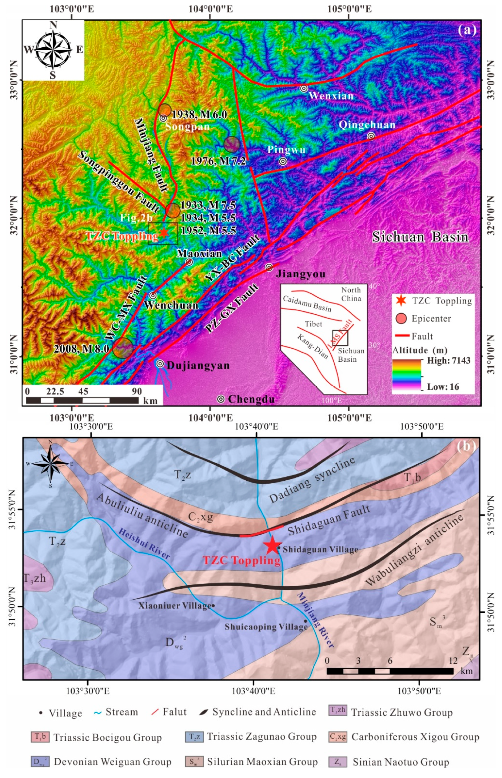
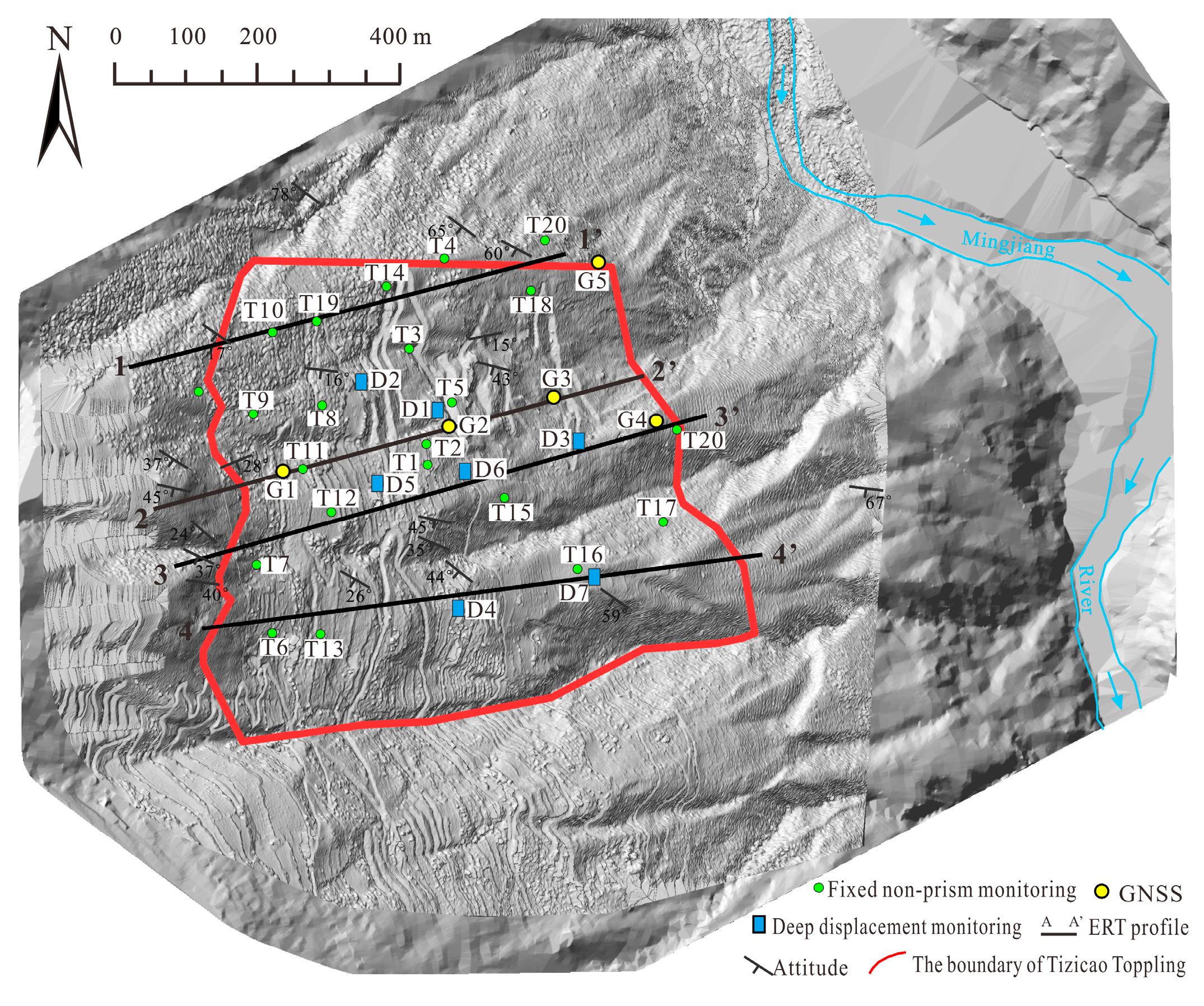
2.1. Study Area

The study area is located in the Longmenshan area at the northwest margin of the Sichuan Basin. As the Indian plate continues to squeeze the Tibetan crust northward, the Longmenshan Fault (LMS Fault) belt has been continuously uplifted and deformed (Figure 1a). Since the late Neogene, the total downcutting has exceeded 2000 m [31,32,33]. The geomorphic and geological setting of the study area is controlled by three NE–SW trending parallel reverse faults: the Wenchuan–Maoxian (WC–MX) Fault, the Pengzhou–Guanxian (PZ–GX) Fault, and the Yingxiu–Beichuan (YX–BC) Fault (Figure 1b). The WC–MX Fault and PZ–GX Fault define the northwest and southeast boundaries of the Longmenshan Fault belt, respectively. The YX–BC Fault, located in the central part of the Longmenshan Fault belt, is the seismogenic fault of the 2008 Wenchuan earthquake. The TZC Toppling is about 50 km away from the YX–BC Fault and about 2 km away from the Shidaguan Fault (Figure 1b). The Shidaguan Fault is developed between the Devonian and Triassic Formations and is a compressional shear fault. The Shidaguan Fault intersects with the Abuliuliu anticline at Shidaguan Village. The Abuliuliu anticline affects the Devonian, Carboniferous, and Triassic strata. The Dadian syncline is located in the northern part of the study area, developed in the Triassic Formation with an arc-shaped axis. The Wabuliangzi anticline is located in the southern part of the study area, developed in the Silurian Formation. The study area belongs to a highly tectonically active zone [34]. Since the last century, six strong earthquakes with magnitudes over 5 have occurred within 200 km of the study area [35] (Figure 1a).
Figure 2 shows the distribution of monthly average rainfall from January 2014 to October 2023 in Maoxian County. In the study area, rainfall is heavy from April to September, accounting for more than 90% of the annual precipitation. Rainfall is low in spring and winter.
The TZC Toppling is located in Shidaguan Township, 35 km northwest of Maoxian County, Sichuan Province (Figure 1). The TZC Toppling is located on the right bank of the Minjiang River flowing through the study area in the north–south direction (Figure 3a). According to the topography, the TZC slope can be divided into three sections (Figure 4): the first section is from the front edge of the toppling to the riverbed (elevation 1750–1960 m), which is the steepest section of the whole slope (average slope 77°); the second section (elevation 2000–2400 m) is mainly the range of the TZC Toppling and is the gentlest section of the slope (average slope 25°); the third section is above the back edge of the toppling, with an average slope of about 47°. Three gullies are developed on the TZC Toppling body: the Large Trough Gully is near the northern boundary, the Nine Turn Gully is in the middle, and the Old Bear Cave Gully is near the right boundary of the toppling (Figure 3b). The crack L01 (Figure 3b) serves as the back edge of the TZC Toppling. The front edge of the toppling (elevation 2020–2040 m) is located at the topographic transition from gentle to steep, and the middle of the front edge is characterized by bulging (L03 in Figure 3b). Feather-shaped shear fractures are mainly developed at the northern boundary of the toppling (L02 in Figure 3b). The length (east–west) of the TZC Toppling is 560 m, the width (north–south) is about 600 m, and the height difference is nearly 400 m.
The field survey collected 129 sets of rock strata and joint production data. Figure 5 shows the orientation information of these rock layers and joints by equatorial projection. The dip direction is determined by an angle of rotation in a clockwise direction starting from the north direction, which is 0°. The dip angle is determined by the equal angle method on the dip direction line with the center of the circle as 0° and the circumference as 90°. The original bedrock layer attitude is N70°W/SW/79° (strike/dip direction/dip) (Figure 5i). The attitude at the front edge is N74°W/SW/67°, which does not vary much from the original bedrock (Figure 5a). The attitude at the central south side is N55°W/SW/56° (Figure 5b), N20°E/SE/45° at the central north side (Figure 5h), and N86°W/SW/45° (Figure 5c) and N74°W/SW/39° (Figure 5d) at the back edge. The dip angle of the bedrock becomes slower from low to high elevation. At the same time, two groups of dominant joints are developed on the slope: J1 (N49°E/SE/73°) is perpendicular to the bedrock and J2 (N18°W/NE/65°) is almost parallel to the valley and tends to be outside the slope (Figure 5c,d). According to the types of cracks and their locations, the toppling is divided into five zones where they occur: Zone I develops tensile cracks (L15 and L16 are shear cracks) with the same orientation as the slope; Zone II includes a staggered north–south and east–west “chessboard-like” tensile failure crack (L03). The widths of the cracks vary from 10 to 50 cm, and the depths of the cracks can be seen to be more than 1 m. Their deformation is characterized by uplifting. Tensile fractures are developed in Zone III. The open distance of L20 is within 60 cm. Zone IV is a highly active area affected by the rock avalanche (Figure 3c) with a maximum length of 355 m and a width of 15 m. The head of the collapse consists of a series of circular tension cracks extending westward from its center. Zone V is characterized by shear cracks oriented parallel to the slope.
The strata exposed in the study area are mainly Devonian Guiguan Upper Group Phyllite, Quaternary landslide deposits, alluvial deposits, and avalanche deposits. The Devonian Guiguan Upper Group Phyllite are 190°∠70°, gray–black, and gray–yellow, as observed at the steep canyon at the front edge.

2.2. Methods

The methods used in this study were designed to collect data from different sources in detail to accurately analyze the deformation evolution of topplings (Figure 6).

2.2.1. On-Site Monitoring
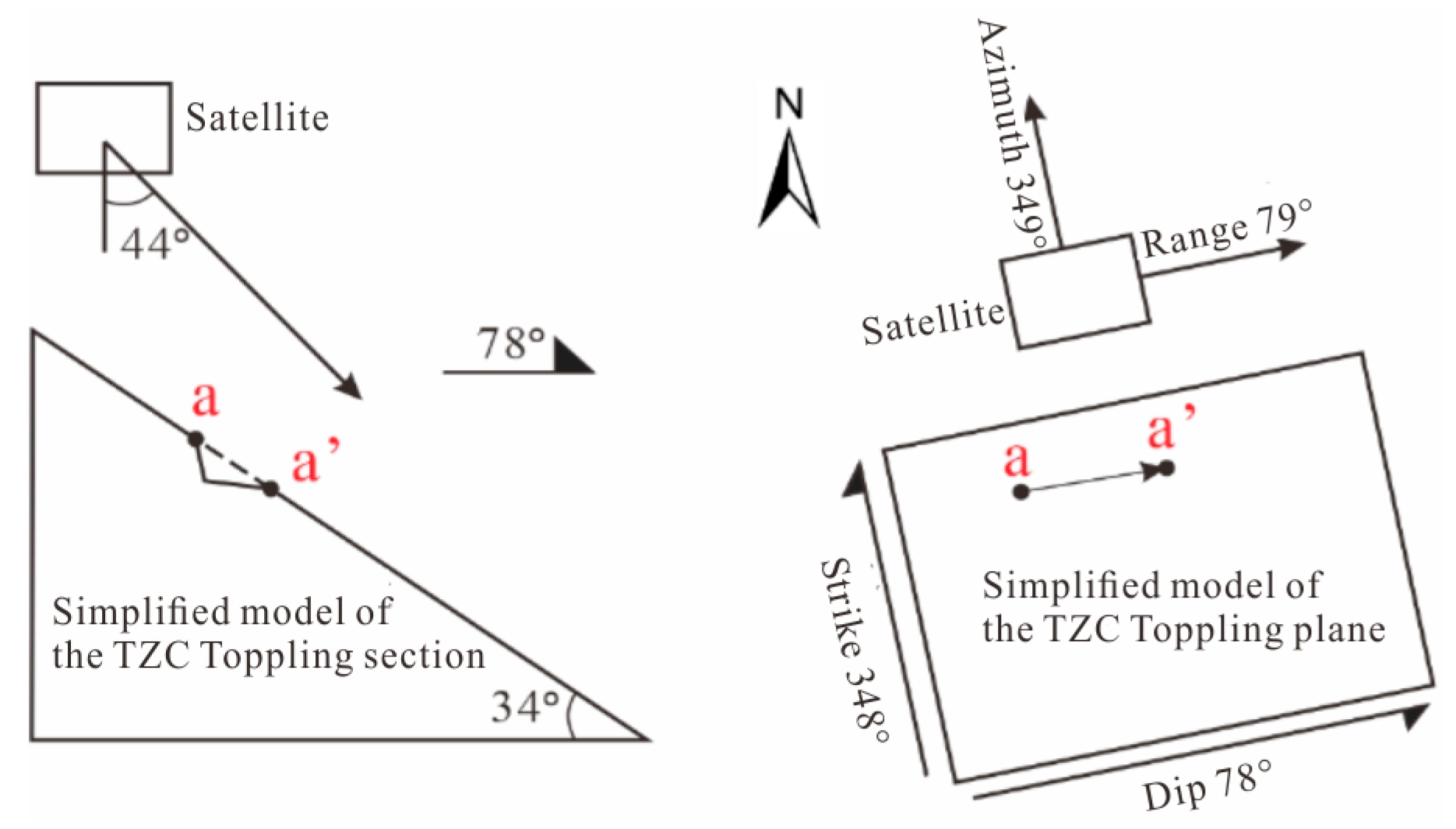
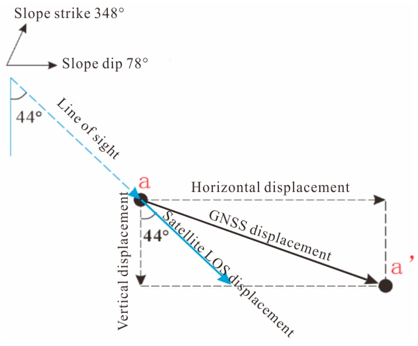
There are a total of 20 fixed non-prism monitoring points on the slope, which are distributed along the 1–1′, 2–2′, 3–3′, and 4–4′ profile lines, and the cumulative resultant displacements from 28 June 2017 to 18 September 2017 were obtained. The deformation information collected from December 2017 to September 2020 was processed and corrected to obtain the cumulative horizontal displacement and cumulative settlement at five GNSS monitoring points, three of which (G1, G2, and G3) were arranged along the 2–2′ profile. Seven deep-displacement-monitoring points acquired depth displacement information from April 2019 to May 2020. In addition, a rainfall-monitoring point was used to monitor the daily surface rainfall. The positions of these monitoring instruments are shown in Figure 7.

2.2.2. SBAS-InSAR

SBAS-InSAR technique is a time series method based on multi-master images [36]. This technique reduces the adverse effects of out-of-coherence and DEM errors and has better applicability and reliability in areas with vegetation cover and in areas with changing ground cover. The ability of the SBAS program to detect the deformation phenomena has been verified in many cases [37,38,39]. In this study, we used 60 Sentinel-1A SAR images acquired in interferometric wide swath (IW) mode and vertical co-polarization (VV) along the ascending orbit. The dataset covers a total period of nearly 24 months, from 2 January 2018 to 11 December 2019. The spatial coverage is shown in Figure 3. The vertical baseline distribution range is 0.5648–262.914 m. The satellite azimuth is 349°. The satellite range is 79°, which intersects with the slope dip at a small angle. The incidence angle in the study area is 44° from the vertical direction (Figure 8). Based on the ENVI platform, data processing was carried out using the SBAS-InSAR method, in which the maximum normal baseline and temporal maximum baseline are 45% and 90 days. In total, 3254 image pairs were obtained by preliminary interference, and the quality of the image pairs was judged and selectively rejected based on the time–position and time–baseline images (Figure 9). The minimum cost flow (MCF) method (Costantini, 1998) with a coherence threshold of 0.2 was used in the differential interference. The correlation coefficient thresholds for the two-step inversion process were set to 0.2 and 0.25, respectively. Finally, the deformation of the TZC Toppling along the satellite LOS direction was obtained by geocoding, and the SBAS-InSAR results were visualized by Matlab 2018 and ArcMap 10.7 software.
The SBAS-InSAR technology monitors the uplift or subsidence of the slope surface along the LOS direction of the remote sensing satellite, which cannot directly reflect the real three-dimensional deformation of the slope surface. However, the deformation data monitored by GNSS is the real deformation in the three-dimensional space of the slope [3]. Therefore, the surface deformation monitoring results of SBAS-InSAR can be further evaluated quantitatively based on GNSS monitoring data. Since the deformation direction of the TZC Toppling is approximately the same as the slope dip, which is 78°, and the satellite range is 79°, when a point on the surface of the toppling moves from a to a′, it can be approximated that the GNSS displacement and the satellite LOS displacement belongs to the same vertical plane with the direction of 78° in space (Figure 10). The measured displacement of GNSS can be decomposed into horizontal displacement and vertical displacement.
Based on the above spatial relationship between the LOS deformation monitored by the satellite and the GNSS deformation in the two-dimensional plane, the equation for the projection of the real vector deformation of the slope surface in the satellite LOS direction is constructed as follows:
S l o s = c o s θ S v ,
S l o s is the projection component of the GNSS displacement in the satellite LOS direction (mm), θ is the incidence angle (°), S v is the actual displacement vertical component (mm). The quality of SBAS-InSAR results is quantitatively evaluated by analyzing the trend and correlation between the projection component of the GNSS displacement in the satellite LOS direction and the satellite LOS displacement based on the Spearman correlation analysis, and the Spearman correlation coefficient r was calculated as:
r = C o v ( R x , R y ) S R x · S R y = i = 1 n ( R x i R x ¯ ) ( R y i R y ¯ ) i = 1 n ( R x i R x ¯ ) 2 ( R y i R y ¯ ) 2 = 1 6 i = 1 n d i 2 n ( n 2 1 )
C o v is the covariance of the two variables, S R x and S R y are the sample speciations, R x i and R y i are the ranks of data i , R x ¯ and R y ¯ are the mean ranks of variables x and y , n is the number of observation pairs, and d i denotes the difference between ranks of x and y .
d i = R x i R y i
The correlation coefficient r between 0.8–1.0 is a very strong correlation, between 0.6–0.8 is a strong correlation, between 0.4–0.6 is a moderate correlation, between 0.2–0.4 is a weak correlation, and 0.0–0.2 is a very weak or no correlation. Sig. is the test value for significant difference and its value being less than 0.05 is considered statistically different, i.e., the null hypothesis is rejected.

2.2.3. Multi-Period Image

Sentinel-1A was launched in April 2014, so data before 2014 are lacking. The deformation values during 2014–2017 exceeded the technical threshold of SBAS-InSAR, resulting in large errors in the processed monitoring data. Therefore, in order to obtain the accurate slope surface deformation, four-view optical images and two unmanned aerial images of the TZC Toppling from 9 January 2010 to 10 May 2020 were collected. The specific parameters of the images are given in Table 1. After the images were pre-processed including geometric correction, the obvious signs within the range of the TZC Toppling were identified as roads through human–machine interaction. The optical image of 9 January 2010 was used as the starting displacement to decode the road displacement of each optical remote sensing image. In this way, the historical deformation of the TZC Toppling from 2010 to 2019 was qualitatively and quantitatively analyzed.

3. Results

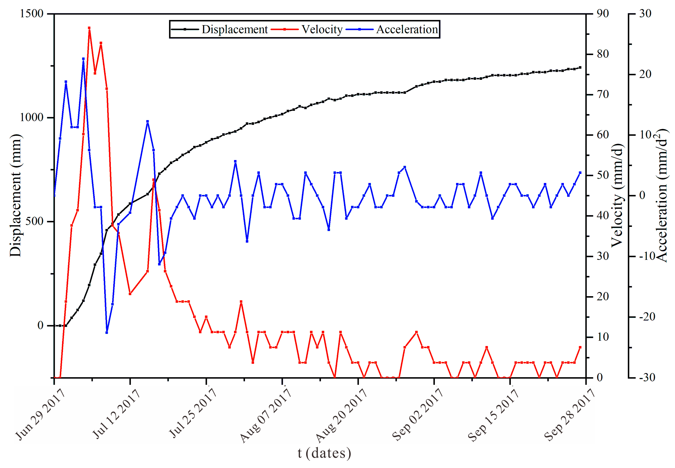
3.1. Real-Time Monitoring Results

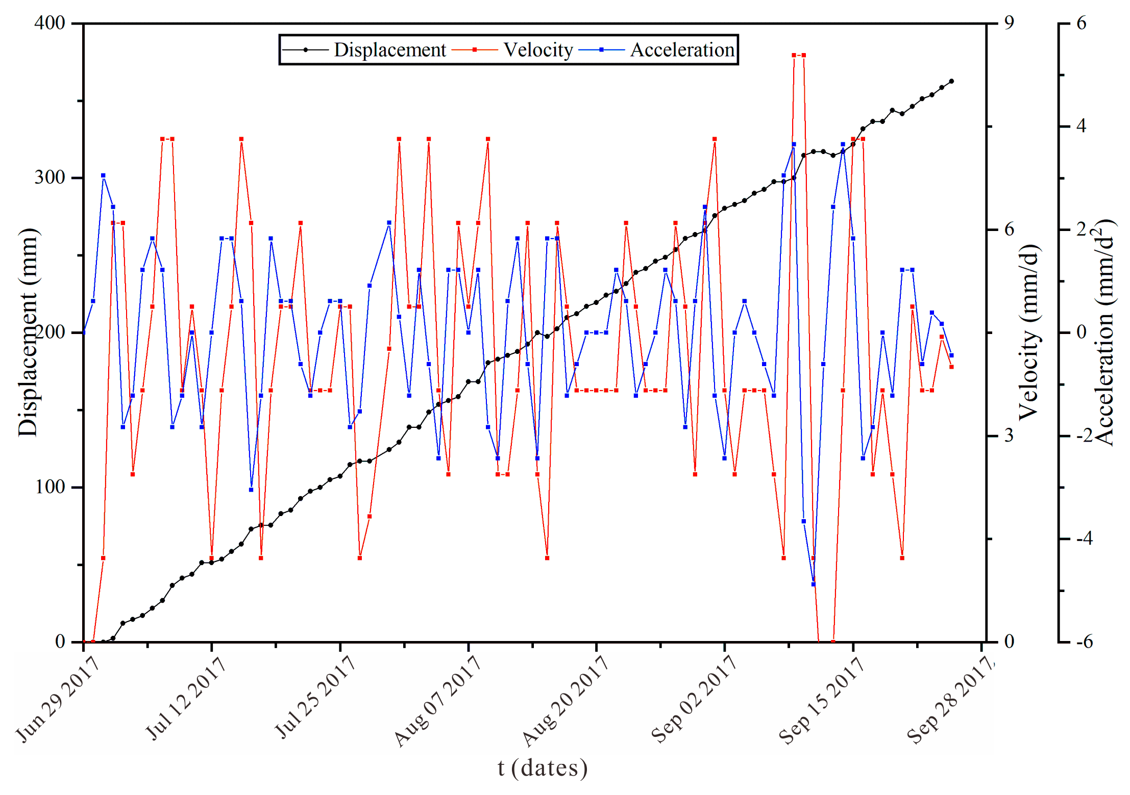
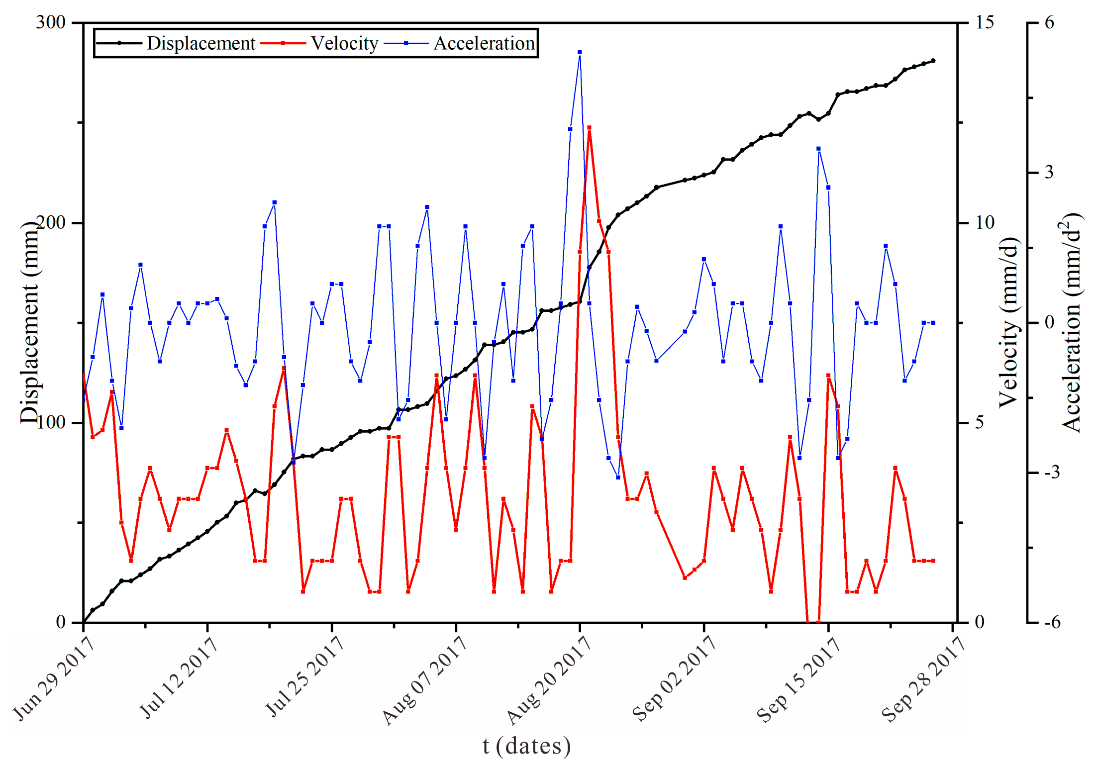
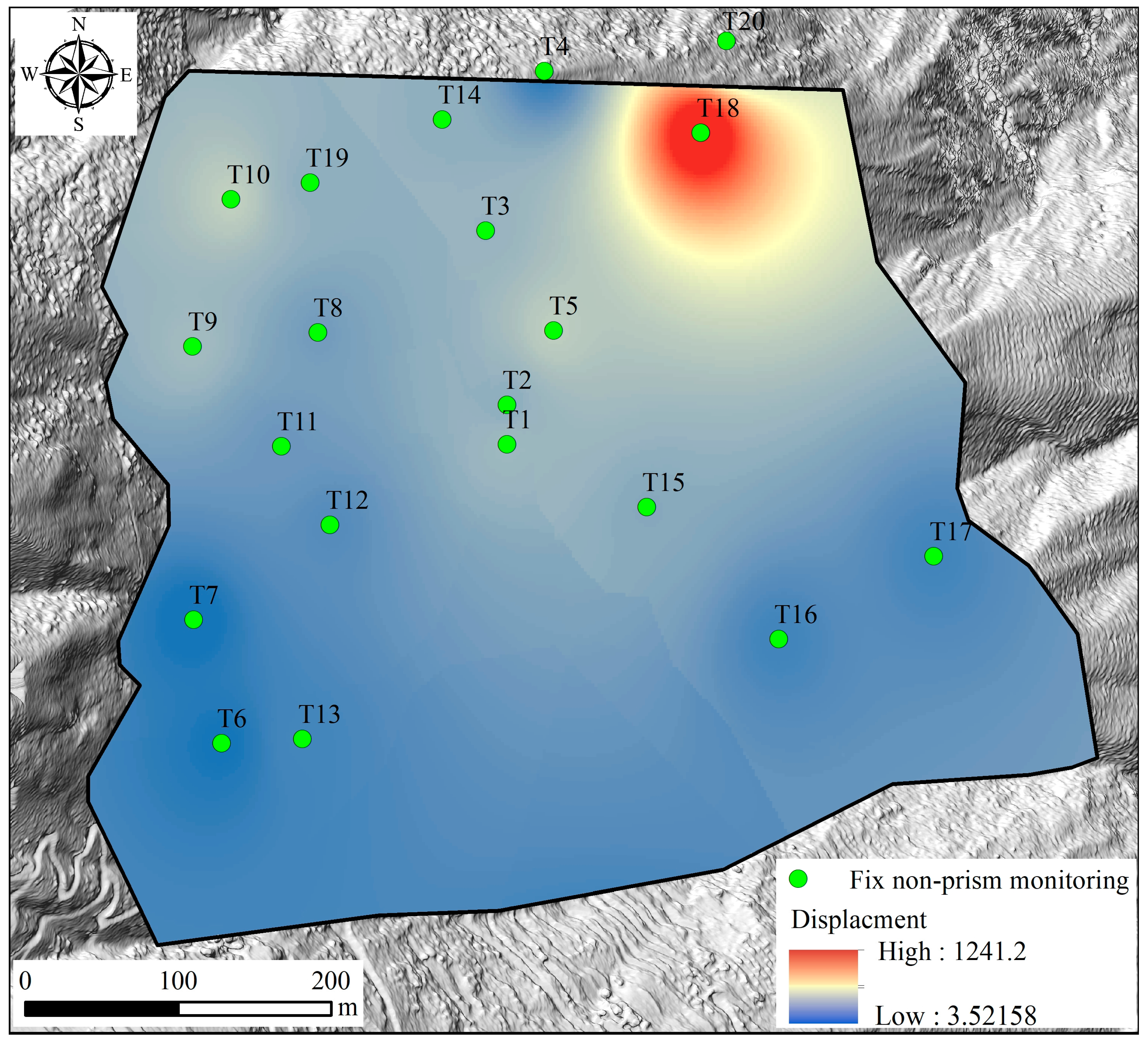
3.1.1. Fixed Non-Prism Monitoring

The fixed non-prism monitoring results revealed that the cumulative displacement on the north side of the TZC Toppling was larger than the value on the south side (Figure 11). The T18 monitoring point had the maximum displacement of 124.19 cm, and the corresponding maximum deformation rate and the maximum deformation acceleration were 86.56 mm/d and 22.58 mm/d2, respectively (Figure 12). The T10 monitoring point had the second largest resultant deformation on the north side of the toppling, which was 36.25 cm, corresponding to the maximum deformation rate and the maximum deformation acceleration of 8.54 mm/d and −4.88 mm/d2 (Figure 13). The T1 monitoring point had the largest resultant deformation on the south side of the toppling, which was 28.10 cm, corresponding to the maximum deformation rate and the maximum deformation acceleration of 12.37 mm/d and 5.41 mm/d2 (Figure 14).

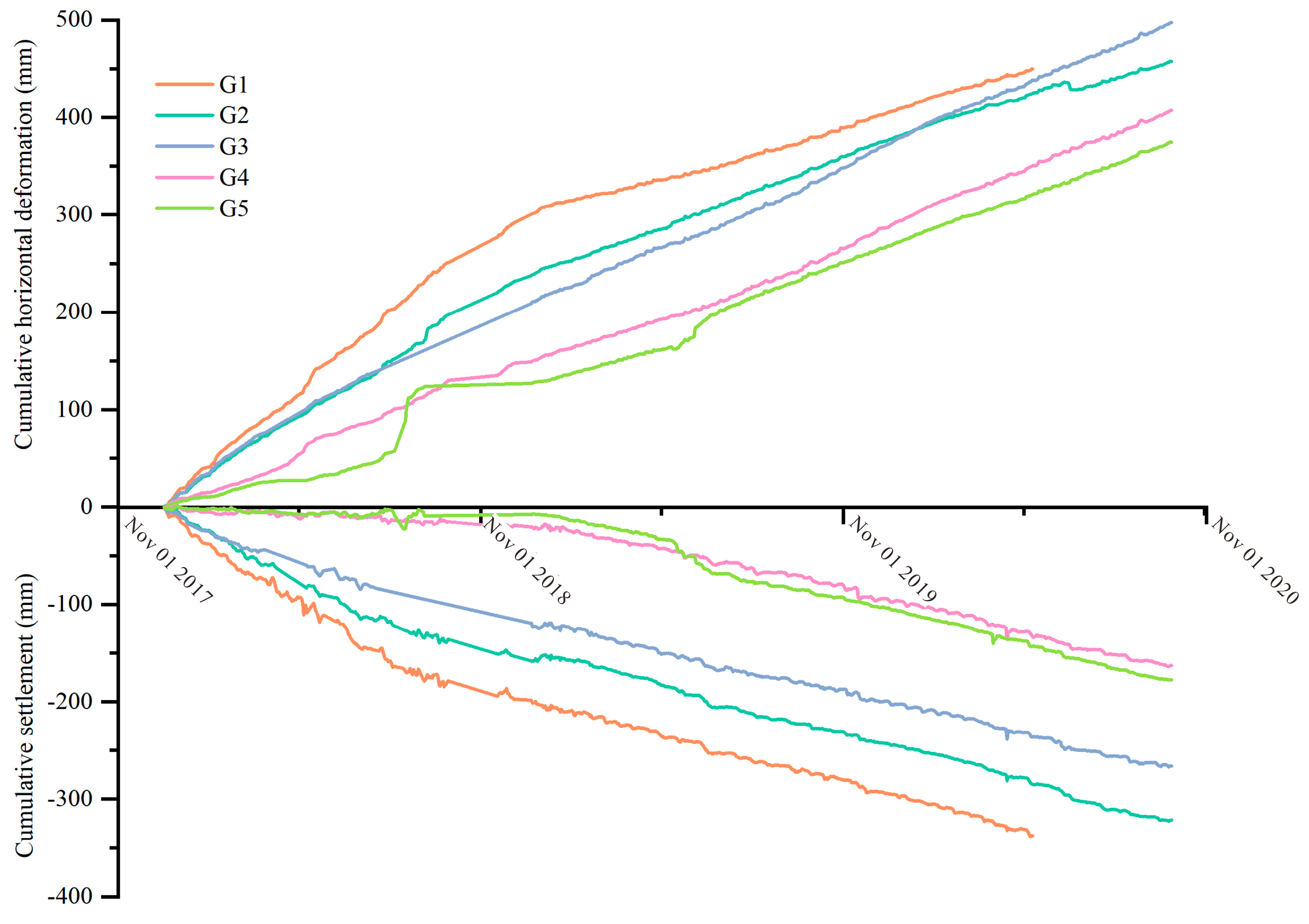
3.1.2. GNSS Monitoring

Figure 15 illustrates the monitoring point with the largest cumulative horizontal displacement and cumulative settlement from 2017 to 2020 is G1, reaching 450.04 mm and 337.33 mm, respectively. Cumulative horizontal displacements and settlements at the three monitoring points arranged along the 2–2′ profile increased with increasing elevation. Moreover, the deformation rates of these three monitoring points slowed down after January 2018 according to the real-time deformation curves. The monitoring point with the smallest horizontal cumulative displacement was G4 located in the middle of the topping with the displacement of 374.61 mm. The monitoring point with the smallest cumulative settlement was G5 located at the boundary of the toppling with the displacement of 162.81 mm.

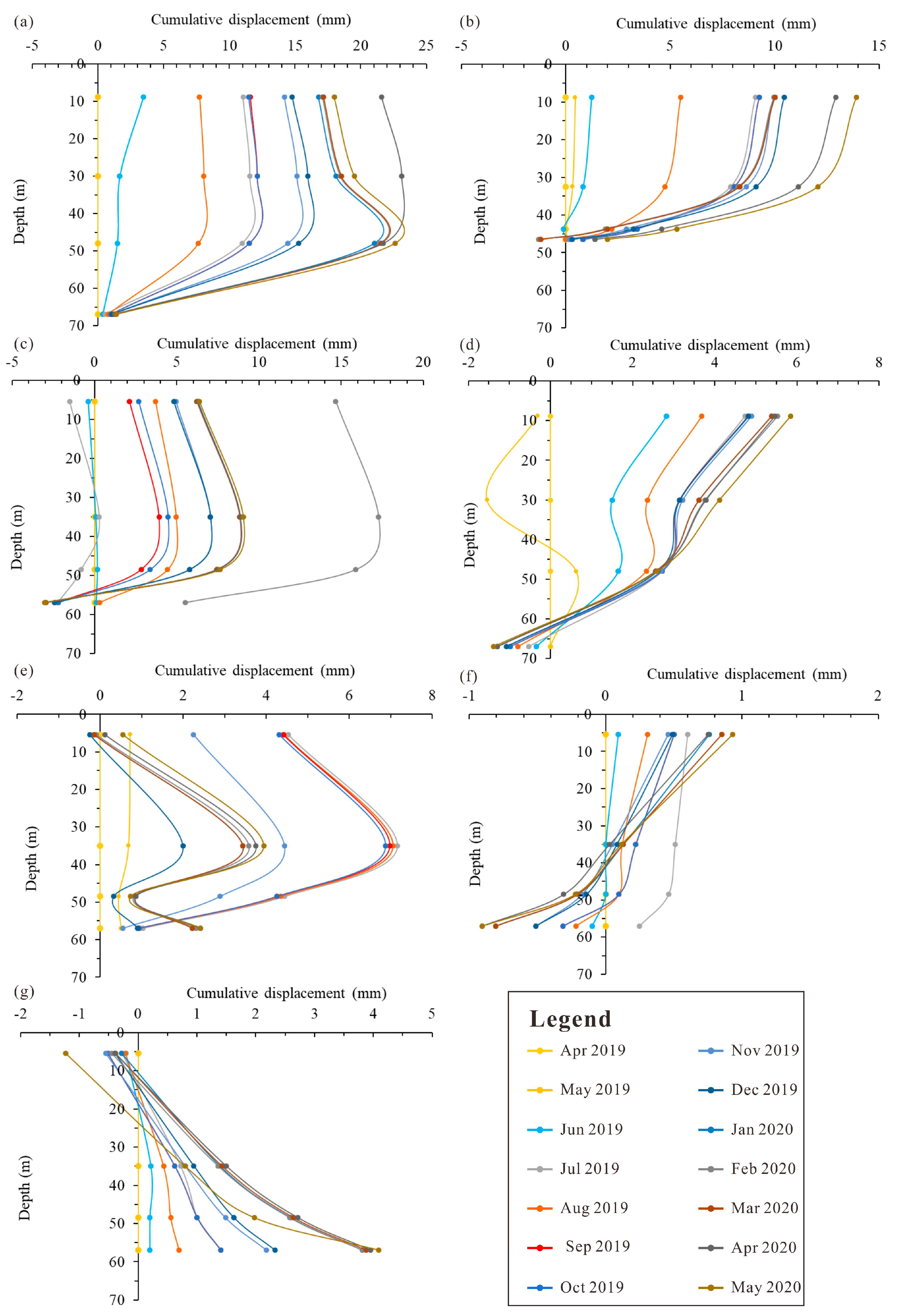
3.1.3. Deep Displacement Monitoring

From April 2019 to May 2020, D1 had the largest cumulative displacement of 23 mm (Figure 16a). This was followed by D2, which is located in the middle of the north side of the toppling, with a cumulative displacement of 17 mm (Figure 16b). D3 is located on the front edge of the toppling and adjacent to the collapse, and its cumulative displacement reached 14 mm (Figure 16c). There was no significant difference in the stratigraphic displacement above the bedrock–cover interface at these three boreholes. The cumulative displacements of D4 and D5 increased by 7 mm (Figure 16d,e). The stratigraphic displacements above the bedrock–cover interface at these two monitoring points differed significantly, and the slope displacement at D4 increased as the depth decreased. The cumulative displacement of D6 and D7 was less than 5 mm (Figure 16f,g).

3.2. SBAS-InSAR Data

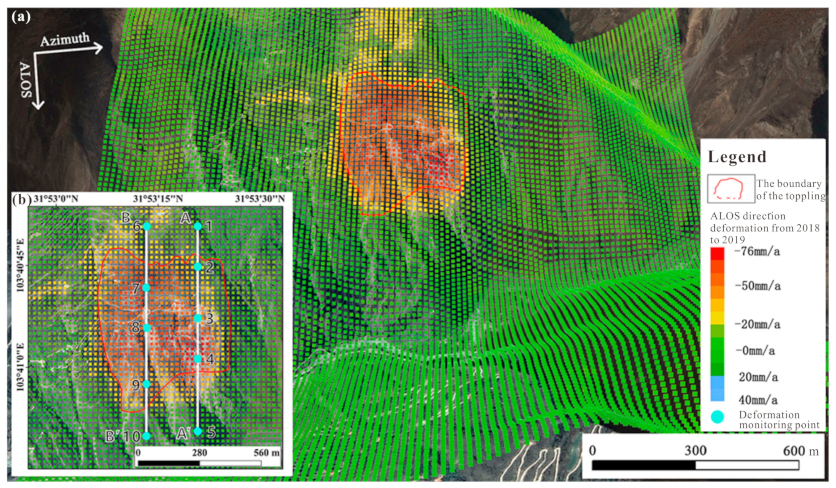
3.2.1. Slope Surface Deformation Monitoring Based on SBAS-InSAR

The preliminary results of the deformation rate were obtained by ENVI 5.3 software. The results of the interferometric treatment were visualized in three dimensions to obtain a map of the annual average rate along the satellite LOS direction in the study area during the time coverage period (Figure 17a). The red line is the boundary of the TZC Toppling. It can be seen in Figure 17a that the settlement rate of the slope exceeding −20 mm/a was mainly concentrated within the red boundary. The deformation rate was the largest around the rock avalanche at the north side of the front edge, where the deformation rate reached −76 mm/a. The highest deformation rates in the upper and middle areas of the toppling reached −70.17 mm/a and −61.06 mm/a, respectively.
Based on the SBAS-InSAR results from 2 January 2018 to 11 December 2019, the cumulative surface deformation of the study area can be extracted (Xie et al., 2020, [13]). A total of 10 monitoring points were selected along profile lines A–A′ and B–B′ (Figure 17b), and the details of the selected points are shown in Table 2.
Taking 2 January 2018 as the starting zero displacement point, the cumulative surface displacement of the TZC Toppling over time was obtained (Figure 18). All monitoring points had no obvious deformation in the first 3 months. Then, the cumulative deformation of points 1, 5, and 10 outside the TZC Toppling remained between ±10 mm, while the monitoring points within the area of the toppling began to deform. As the elevation increased, the cumulative deformation at the monitoring points arranged along the A–A′ profile inside the toppling became smaller, and the maximum cumulative deformation at point 4 was −152.86 mm. As the elevation increased, the cumulative deformation at the monitoring points arranged along the B–B′ profile inside the toppling became larger, and the cumulative settlement deformation at point 7 reached −140.34 mm.

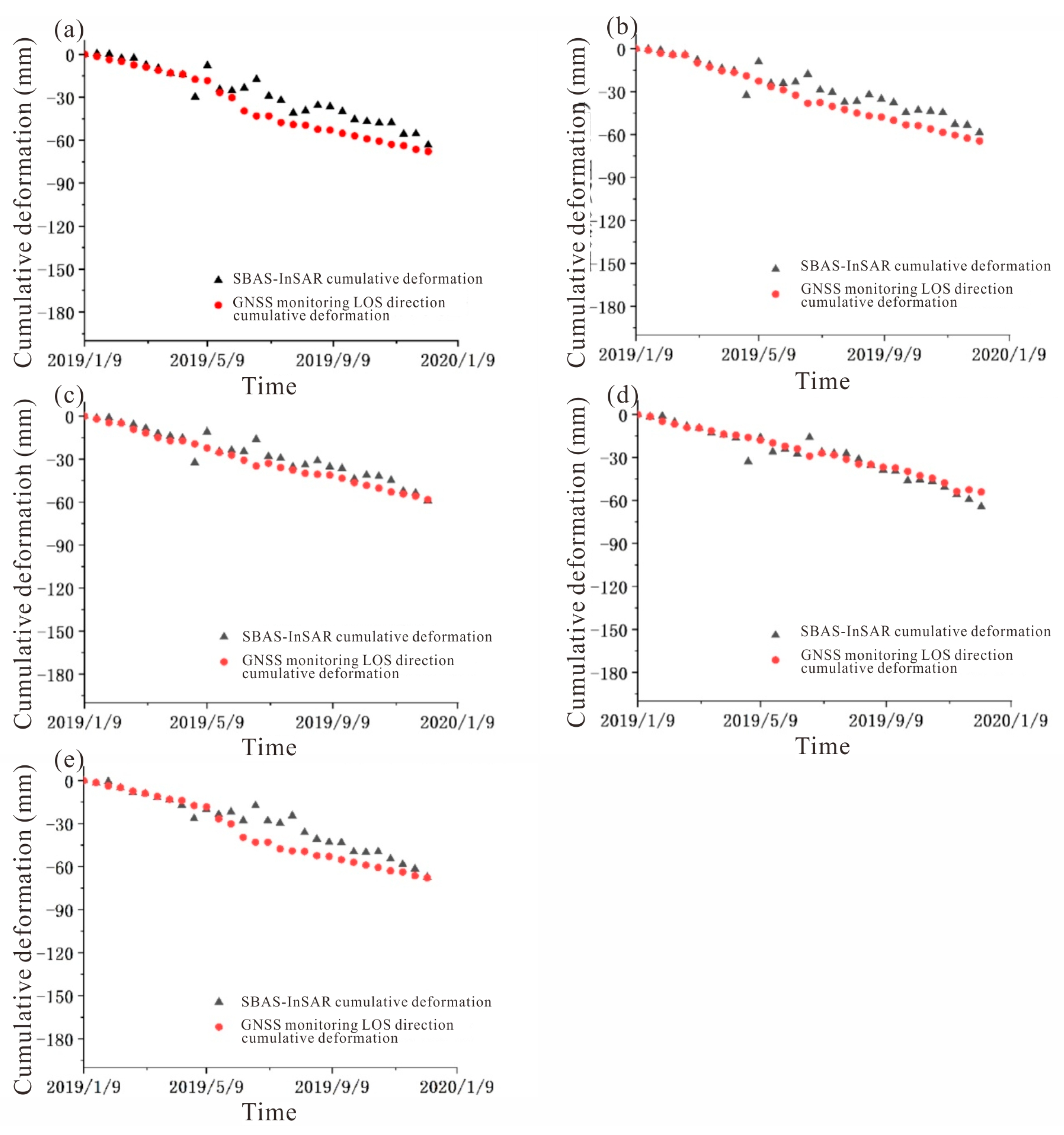
3.2.2. Precision of SBAS-InSAR

In the comparative analysis, the displacement measured by GNSS monitoring points was projected to the satellite LOS direction, and the deformation time series along the LOS direction were obtained.
Taking 1 January 2019 as the unified reference zero reference time of the InSAR monitoring and GNSS monitoring deformation series, the average value of deformation of all InSAR monitoring points within a 50 m radius of the GNSS monitoring point was compared with the GNSS monitoring results along the LOS direction (Figure 19). The changing trend of the cumulative deformation obtained by the two monitoring methods was similar. The difference in the cumulative deformation obtained by the two methods ranged from 0 to 15 mm, while the maximum difference reached 25 mm only at G5.
Using the Spearman correlation analysis method to analyze the deformation values obtained by both methods, the results showed that the sig. was less than 0.05 and the correlation coefficient was greater than 0.94 (Table 3). Thus, the GNSS monitoring deformation along the LOS direction was in significant agreement with the SBAS-InSAR results.

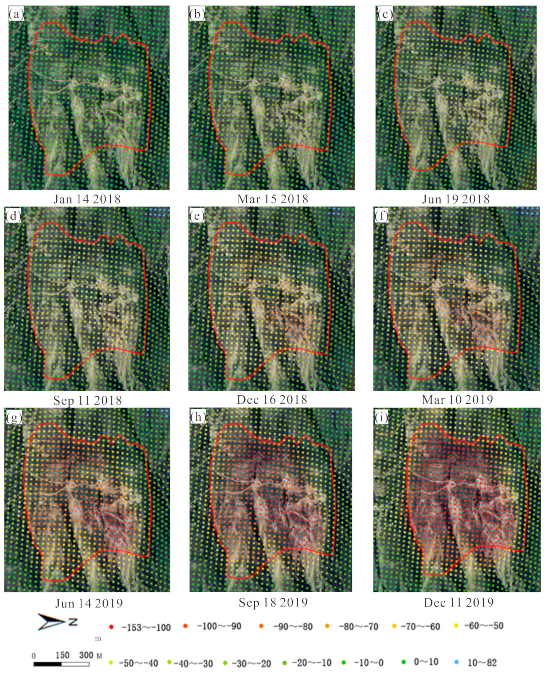
3.3. Multi-Phase Image Data

According to the optical image (Figure 20a), exposed rock mass that is large in scale and in contrast to the color and morphology of the surrounding rock mass is visible at the leading edge of the TZC Toppling, and there is collapsed material in the river below. It can be determined that a rock avalanche has occurred in this area historically. In 2010 and 2011, no obvious signs of deformation were seen in the middle and front edge of the toppling (Figure 20a,b). From 2011 to 2016, the deformation increased significantly, the north side of the front edge of the toppling was destabilized and collapsed, the tension cracks at the rear edge gradually expanded and penetrated, obvious bulging and fractures were shown at the center front edge, and a set of plume-shaped cracks were distributed at the north boundary (Figure 20c). From 2016 to 2017, the tension cracks on the trailing edge continued to widen, forming a table can with a maximum width of about 8 m. The range of the rock avalanche on the north side of the leading edge gradually expanded to the middle of the toppling, forming several tension cracks. The bulging cracks on the south side of the leading edge also have some expansion. The north boundary crack is extended through and gradually connected with the back edge tension crack (Figure 20d). After 2017, the deformation of the TZC Toppling converged and no new obvious cracks were produced (Figure 20e,f).
To further quantify the historical deformation of the TZC Toppling, we used five phases of high-precision optical remote sensing images on 9 January 2010, 17 March 2011, 25 December 2011, 9 January 2016, and 23 October 2019. The landmark roads on these images, which were corrected and aligned, were interpreted, and the multi-period interpretation results were superimposed to obtain the deformation of the toppling during 2010–2019 (Figure 21).
A large-scale rock avalanche occurred at the north front edge of the toppling. By 23 October 2019, the range of the rock avalanche had exceeded 1 km2, and the roads within the range were completely destroyed. The cumulative displacement of the middle of the north side of the toppling from 2016 to 2019 exceeded 12 m, reaching a maximum of 27.2 m. Compared with the strongly deformed area, the deformation of the middle of the toppling was smaller, only 5–8 m. The closer to the front edge, the larger the deformation, up to 12.5 m, and the closer to the north side, the greater the deformation. The deformation of the south side of the toppling was the smallest, the deformation was 0–2.5 m without obvious signs of displacement before 2016, and the maximum cumulative deformation only reached 5 m as of 2019.

4. Discussion

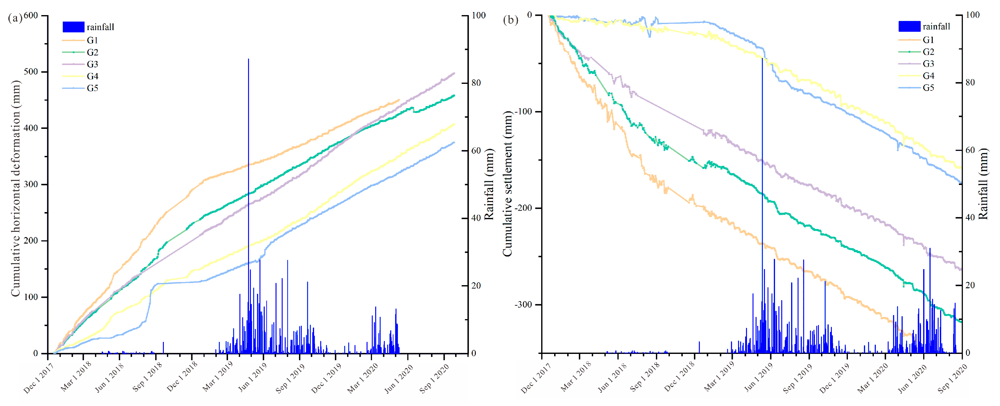
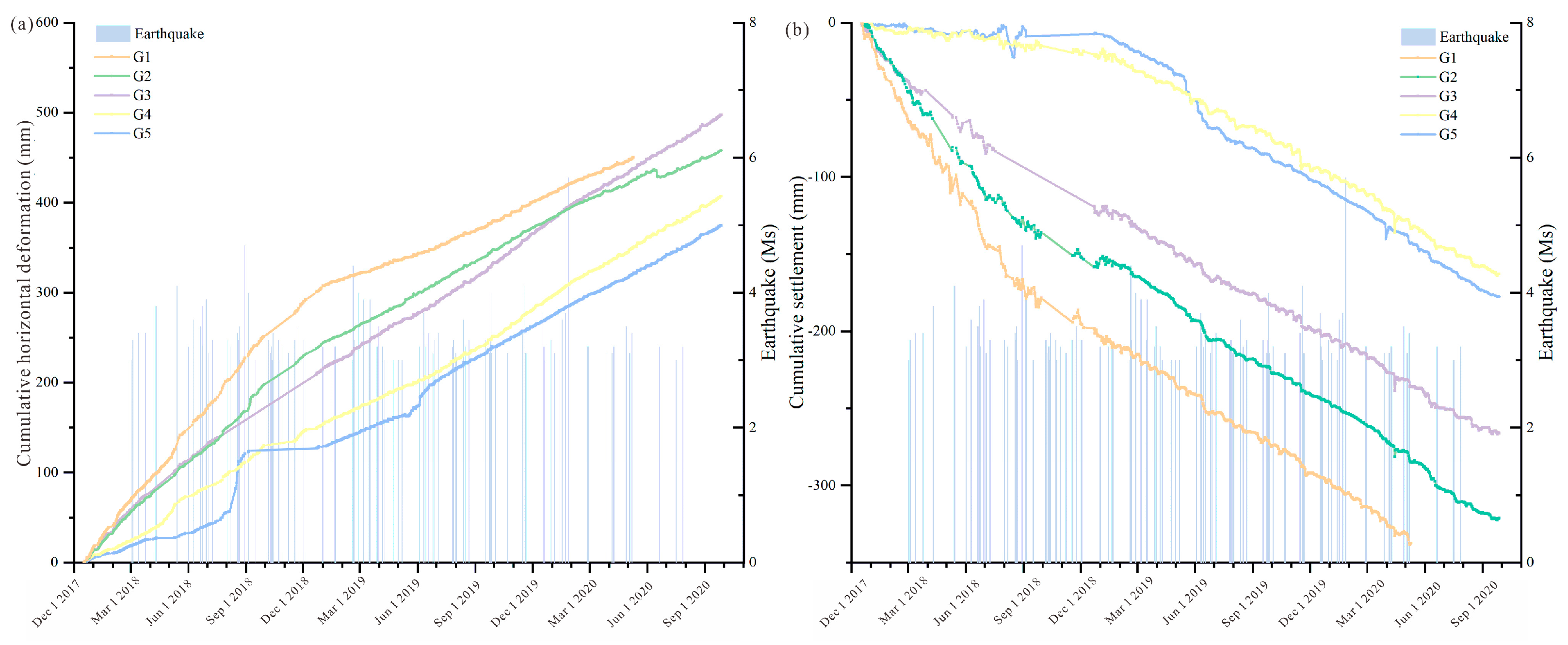
4.1. Spatio-Temporal Deformation Evolutionary Characteristics

According to the historical multi-phase optical images (Figure 20 and Figure 21), the TZC Toppling began to deform in 2010, and the deformation rate was slow. In 2014, a rock avalanche occurred at the north side of the leading edge, and deposits with a volume of nearly 6 × 10⁴ m3 washed into the Minjiang River, occupying nearly 1/3 of the river channel. Cracks appeared on the rear edge and the north side of the dump. In the middle of the front edge, there are “chessboard-shaped” cracks that crisscross from north to south and from east to west. In 2017, a through crack appeared at the rear edge and was staggered for more than 10 m. Then, the deformation of the toppling began to converge without any significant new cracks. No obvious settlement occurred in the first three months of 2018 (Figure 22a,b). It was not until June 2018 that settlement began to occur near the rock avalanche (Figure 22c). Then, the deformation range increased (Figure 22d). In December 2018, the cumulative deformation along the satellite LOS direction reached a maximum of −80 mm (Figure 22e). At the same time, the deformation range of the toppling gradually expanded from the north side of the front edge to the back edge and the south side, and the cumulative deformation in the upper south side reached -65 mm. From December 2018 to December 2019 (Figure 22f,g–i), not only did the cumulative deformation of the upper south side and the north leading edge increase continuously, but the cumulative deformation of the central part was also gradually increased by the influence of the north front edge. The temporal deformation evolution characteristics of the toppling were obtained by combining the historical multi-phase optical images and SBAS-InSAR results.
We also found that there were spatial differences in the deformation of the TZC Toppling. Through unmanned aerial vehicle images taken on 10 May 2020, it seems that more, wider, and longer cracks developed on the upstream side of the toppling than on the downstream side. From the upstream side to the downstream side, the number of cracks decreased from 14 to 7, and the type of cracks changed from shear to bulge. In December 2019, the maximum cumulative deformation of the north side of the leading edge reached a maximum of −150 mm, the maximum cumulative deformation of the upper side was more than −100 mm, and the deformation of the south side of the leading edge was less than −100 mm (Figure 22). In order to investigate the spatial deformation evolution of the toppling, the interpolated cloud map of deformation was drawn using the data obtained from 20 fixed non-prism monitoring points (Figure 23). According to Figure 23, it can be seen that the maximum displacement occurred on the north side of the toppling (T18), close to the rock avalanche, and the cumulative displacement reached 1241.9 mm. The surface displacement in the upper part was 100–350 mm. The minimum displacement occurred in the southside, and the cumulative surface deformation was less than 100 mm.
From April 2019 to May 2020, the monitoring point with the largest cumulative deep displacement was D1 located at the north leading edge, followed by D4 and D5 located at the upper south side, and the monitoring points with the smallest cumulative deep displacement were D6 and D7 located at the lower south side of the dumping body (Figure 16). The SBAS-InSAR data, deep displacement data, and slope surface displacement data are consistent. The rock avalanche occurs at the north side of the leading edge to form tension cracks, where the displacement is the largest. Under the influence of sliding traction at the northern leading edge, the upper part of the toppling formed a tensile stress concentration zone and formed tension cracks, while the lower part of the south side of the toppling was extruded and compression-tension cracks were formed with minimum displacement.
The long-term comprehensive remote sensing interpretation and short-term real-time monitoring revealed the spatial and temporal deformation evolution process of the TZC Toppling. However, it is still a debatable issue as to what evolution stage the TZC Toppling is currently in and whether it will suddenly fracture after such a long period of deformation evolution. In order to accurately determine what stage the toppling is currently in, we adopted the acceleration threshold method [40] for the slope with slow creep characteristics. According to Figure 12, Figure 13 and Figure 14, all three monitoring points revealed that the acceleration fluctuated around 0 mm/d2, so the toppling was in the constant deformation stage and did not enter the acceleration deformation stage (Figure 24). However, since the monitoring data in this study only went up to September 2020, it was impossible to determine whether the TZC Toppling is currently in the initial accelerated deformation stage. According to the borehole information in the previous study [41], a layer of silty clay with an RQD value of 0 was found at the bedrock–cover interface of the toppling. According to the electron microscope scanning image, slickensides were found at the bedrock–cover interface on the north side of the toppling (Figure 25a), while the slickensides at the bedrock–cover interface on the south side were characterized as arc-shaped (Figure 25b), which were caused by creeping friction. In addition, the ERT results [41] showed that the fracture zone on the south side of the toppling was stepped. The evidence showed that the south side of the toppling was in the toppling–bending deformation stage. This does not mean that the toppling was in the acceleration deformation stage, even if the surface displacement was large. It needs to be combined with the acceleration threshold method and the subsurface structure to make a comprehensive judgment (Figure 24).

4.2. Deformation Sensitivity

In order to analyze the effects of earthquakes and rainfall on the deformation of the TZC Toppling, we used displacement data and corresponding earthquake and rainfall data. Figure 26 shows the monitored rainfall data from 17 December 2017 to 21 July 2022. The rainfall from 2019 to 2021 was greater than that of 2018 and 2022. The largest amount of rainfall was recorded in 2019, with the greatest rainfall of 87.2 mm on 12 May 2019. It is known from Section 3.2.2 that the historical deformation data extracted based on SBAS-InSAR and GNSS monitoring data have high consistency, but the GNSS monitoring time is longer, so GNSS monitoring data were used to perform the analysis. According to Figure 26, the accumulated deformation of the toppling varied with the rainfall in the rainy season, while the deformation presented nearly uniform deformation during the non-rainy season. After the toppling experienced the maximum rainfall of 87.2 mm during the monitoring period, the cumulative settlement at the five GNSS monitoring points showed significant increases after about 15 days, and the cumulative horizontal displacement at G5 showed a significant increase after 15 days. Then, the toppling resumed a relatively uniform deformation. According to Figure 27, the response of the dumped body to earthquakes from 2017 to 2020 was weak.
In order to clarify the effects of rainfall and earthquake on the deformation of the TZC Toppling, we conducted the Spearman correlation analysis of the GNSS displacements with rainfall and earthquakes, respectively. According to the results of the correlation analysis (Table 4), the deformation was weakly correlated with rainfall, and the data were significant but extremely weakly correlated or uncorrelated with micro-earthquakes, with no statistical difference.

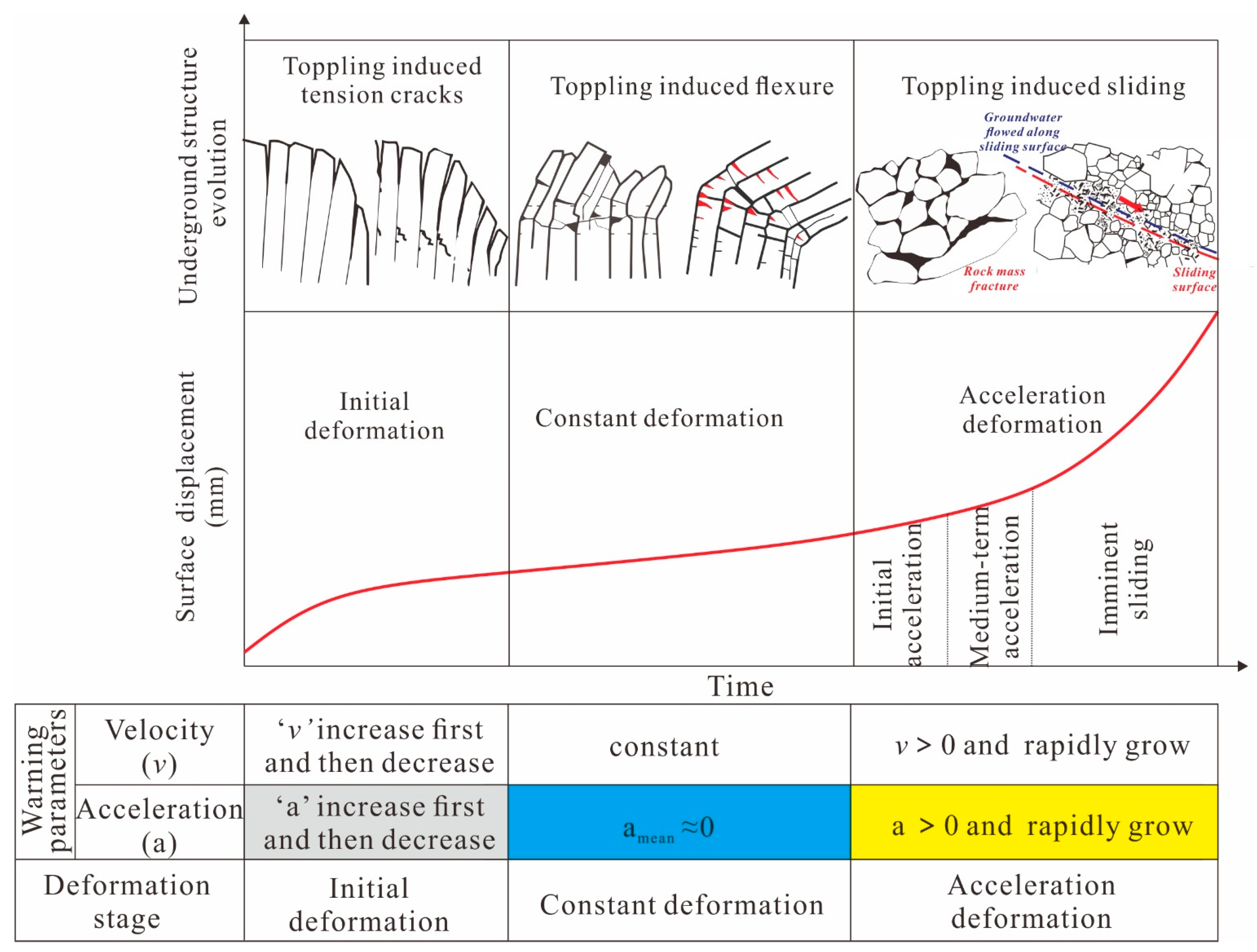
4.3. Geological Model

The TZC Toppling has undergone a long geodynamic development process of downcutting of the Minjiang River valley, unloading of the rock on the reverse slope, toppling–bending, and finally fracture. In this process, the undercutting of the Minjiang River and the lateral erosion of the river has caused the northern side of the toppling to have a good proximity condition. In contrast, the southern front edge has developed with a wide and gentle mountain beam, and this topography improves the stability of the southern slope. According to Figure 5, the tensile fracture (L20) is developed on the front edge of Zone III between the Nine Turn Gully and the Old Bear Cave Gully. The dislocation distance is within 60 cm due to the obstruction of the mountain beams at the front edge. A series of east–west and north–south curved tensile cracks represent the damage in Zone II. The deformation is characterized by uplifting. The width of the cracks varies from 10 to 50 cm, and the depth is more than 1 m. The deformation in Zone II is dominated by the rock avalanche and cracks located at the trailing edge of this zone. The maximum dislocation distance in this zone is 40 m. So, the reason why the deformation tends to be self-stabilizing is inferred to be the existence of the internal structural connection between the north and south parts of the toppling. For the north of the toppling, the rock avalanche occurred at the leading edge, and the deformation range gradually extended to the upper part (Figure 22), forming multiple tensile cracks (L11 and L12 in Figure 5). For the south of the toppling, the tensile stress is concentrated in the upper part and tensile cracks occurred (L08 in Figure 5); the deformation in the upper part is larger than that in the lower part (Figure 18b), and the lower part was squeezed to form obvious bulging cracks (L03 in Figure 5). Therefore, there is a compound evolution mechanism of the TZC Toppling (Figure 28).
The TZC Toppling will enter the overall slip phase after inversion shear occurs in the bulge–cracking part, at which time the overall slope will be initiated. It is known that the TZC Toppling is located in the Minjiang Fault zone. Earthquakes will lead to slope damage on the downstream side, causing the toppling to enter a state of limited equilibrium. So, rainfall and earthquakes will cause the toppling to enter the stage of total slip. Therefore, it is recommended that long-term subsurface and surface deformation monitoring be implemented at the front part of its downstream slope.

5. Conclusions

Deep, unstable slopes especially develop in the Minjiang River Basin, and the TZC Topping is located in Mao County, Sichuan Province, on the right bank of the Minjiang River. The Toppling threatens the safety of 6 households and 30 people on the slope, as well as facilities at the foot of the slope, including the Shidaguan township government, the elementary school, the police station, the gas station, and the G213 national highway, which is the only highway from Wenchuan to Mao County. Therefore, it is important to determine the evolution process of the TZC Toppling. We collected SBAS-InSAR data and optical remote sensing images, and installed real-time monitoring equipment to introduce the main spatial and temporal characteristics of the TZC Toppling. The toppling has undergone an evolution process from increasing deformation to convergence, with the leading edge exhibiting a composite failure mode of “collapse failure” and “bulging cracking”. Furthermore, the correlation between rainfall, earthquakes, and GNSS time series shows that the displacement deformation of the toppling is influenced by rainfall, but the impact of earthquakes is not significant. It is suggested that multi-phase geophysical methods could be carried out to detect the internal structure of the TZC Toppling, so that disaster prevention and mitigation work can be carried out in time once a sudden change in the rock structure is detected.

Author Contributions

All authors significantly contributed to the research. Methodology and investigation, H.W.; resources, X.P. and B.Z.; data curation, L.L. and T.J.; writing—original draft preparation, H.W.; writing—review and editing, S.C. and H.W.; supervision, X.P.; funding acquisition, X.P. and S.C. All authors have read and agreed to the published version of the manuscript.

Funding

This research was funded by the National Key R&D Program of China, grant number 2023YFC3007104, the National Natural Science Foundation of China, grant number 41931296, the State Key Laboratory of Geohazard Prevention and Geoenvironment Pro-tection Independent Research Project, grant number SKLGP2021Z014, and the Sichuan Science and Technology Program, grant number 2022NSFSC1121. H.W. would like to thank the China Scholarship Council (CSC) for funding hisresearch period at the University of Twente (grant number 202309230007).

Data Availability Statement

The processed data required to reproduce these findings cannot be shared at this time as the data also forms part of an ongoing study.

Conflicts of Interest

The authors declare no conflict of interest.

References

  1. Cui, S.H.; Pei, X.J.; Jiang, Y.; Wang, G.H.; Fan, X.M.; Yang, Q.W.; Huang, R.Q. Liquefaction within a bedding fault: Understanding the initiation and movement of the Daguangbao landslide triggered by the 2008 Wenchuan Earthquake (Ms = 8.0). Eng. Geol. 2021, 295, 106455. [Google Scholar] [CrossRef]
  2. Huang, R. Mechanisms of large-scale landslides in China. Bull. Eng. Geol. Environ. 2012, 71, 161–170. [Google Scholar] [CrossRef]
  3. Cenni, N.; Fiaschi, S.; Fabris, M. Integrated use of archival aerial photogrammetry, GNSS, and InSAR data for the monitoring of the Patigno landslide (Northern Apennines, Italy). Landslides 2021, 18, 2247–2263. [Google Scholar] [CrossRef]
  4. Eberhardt, E.; Watson, A.D.; Loew, S. Improving the interpretation ofslopemonitoring and early warning data through better understanding of complex deep-seated landslide failure mechanisms. In Landslides and Engineered Slopes: From the Past to the Future; Chen, Z., Zhang, J., Li, Z., Wu, F., Ho, K., Eds.; Taylor & Francis: London, UK, 2008; pp. 39–51. [Google Scholar]
  5. Irfan, M.; Uchimura, T.; Chen, Y. Effects of soil deformation and saturation on elastic wave velocities in relation to prediction of rain-induced landslides. Eng. Geol. 2017, 230, 84–94. [Google Scholar] [CrossRef]
  6. Shou, K.J.; Wang, C.F. Analysis of the Chiufengershan landslide triggered by the 1999 Chi-Chi earthquake in Taiwan. Eng. Geol. 2003, 68, 237–250. [Google Scholar] [CrossRef]
  7. Tang, H.; Liu, X.; Hu, X.; Griffiths, D.V. Evaluation of landslide mechanisms characterized by high-speed mass ejection and long-run-out based on events following theWenchuan earthquake. Eng. Geol. 2015, 194, 12–24. [Google Scholar] [CrossRef]
  8. Huang, R.Q. Some catastrophic landslides since the twentieth century in the southwest of China. Landslides 2009, 6, 69–81. [Google Scholar]
  9. Sun, H.; Wu, X.; Wang, D.; Xu, H.; Liang, X.; Shang, Y. Analysis of deformation mechanism of landslide in complex geological conditions. Bull. Eng. Geol. Environ. 2019, 78, 4311–4323. [Google Scholar] [CrossRef]
  10. Song, H.F.; Cui, W. A large-scale colluvial landslide caused by multiple factors: Mechanism analysis and phased stabilization. Landslides 2016, 13, 321–335. [Google Scholar] [CrossRef]
  11. Zangerl, C.; Eberhardt, E.; Perzlmaier, S. Kinematic behaviour and velocity characteristics of a complex deep-seated crystalline rockslide system in relation to its interaction with a dam reservoir. Eng. Geol. 2010, 112, 53–67. [Google Scholar] [CrossRef]
  12. Vallet, A.; Charlier, J.B.; Fabbri, O.; Bertrand, C.; Carry, N.; Mudry, J. Functioning and precipitation-displacement modelling of rainfall-induced deep-seated landslides subject to creep deformation. Landslides 2015, 13, 653–670. [Google Scholar] [CrossRef]
  13. Xie, M.L.; Zhao, W.H.; Ju, N.P.; He, C.; Huang, H.; Cui, Q. Landslide evolution assessment based on InSAR and real-time monitoring of a large reactivated landslide, Wenchuan, China. Eng. Geol. 2020, 277, 105781. [Google Scholar] [CrossRef]
  14. Cina, A.; Piras, M. Performance of low-cost GNSS receiver for landslides monitoring: Test and results, Geomatics. Nat. Hazards Risk 2015, 6, 497–514. [Google Scholar] [CrossRef]
  15. Li, M.; Zhang, L.; Dong, J.; Tang, M.; Shi, X.; Liao, M.; Xu, Q. Characterization of pre- and post-failure displacements of the Huangnibazi landslide in Li County with multi-source satellite observations. Eng. Geol. 2019, 257, 105140. [Google Scholar] [CrossRef]
  16. Farina, P.; Colombo, D.; Fumagalli, A.; Marks, F.; Moretti, S. Permanent scatterers for landslide investigations: Outcomes from the ERS-SLAM project. Eng. Geol. 2006, 88, 200–217. [Google Scholar] [CrossRef]
  17. Bulmer, M.H.; Petley, D.N.; Murphy, W.; Mantovani, F. Detecting slope deformation using two-pass differential interferometry: Implications for landslide studies on Earth and other planetary bodies. J. Geophys. Res. 2006, 111, E06S16. [Google Scholar] [CrossRef]
  18. Cascini, L.; Fornaro, G.; Peduto, D. Advanced low- and full-resolution DInSAR map generation for slow-moving landslide analysis at different scales. Eng. Geol. 2010, 112, 29–42. [Google Scholar] [CrossRef]
  19. Zhao, C.Y.; Lu, Z.; Zhang, Q.; Fuente, J.D.L. Large-area landslides detection and monitoring with ALOS/PALSAR imagery data over Northern California and Southern Oregon, USA. Remote Sens. Environ. 2012, 124, 348–359. [Google Scholar] [CrossRef]
  20. Hilley, G.E.; Burgmann, R.; Ferretti, A.; Novali, F.; Rocca, F. Dynamics of slow-moving landslides from permanent scatterer analysis. Science 2004, 304, 1952–1955. [Google Scholar] [CrossRef] [PubMed]
  21. Roering, J.J.; Stimely, L.L.; Mackey, B.H.; Schmidt, D.A. Using DInSAR, airborne LiDAR, and archival air photos to quantify landsliding and sediment transport. Geophys. Res. Lett. 2009, 36, L19402. [Google Scholar] [CrossRef]
  22. Stimely, L.L. Characterizing Landslide Movement at the Boulder Creek Earthflow, Northern California, Using L-Band InSAR. Master’s Thesis, Department of Geological Sciences, Graduate School of the University of Oregon, Eugene, OR, USA, 2009. [Google Scholar]
  23. Calabro, M.D.; Schmidt, D.A.; Roering, J.J. An examination of seasonal deformation at the Portuguese Bend landslide, southern California, using radar interferometry. J. Geophys. Res. 2010, 115, F02020. [Google Scholar] [CrossRef]
  24. Xia, Y.; Kaufmann, H.; Guo, X.F. Landslide monitoring in the Three Gorges area using D-INSAR and corner reflectors. Photogramm. Eng. Remote Sens. 2004, 70, 1167–1172. [Google Scholar]
  25. Fu, X.; Guo, H.; Tian, Q.; Guo, X. Landslide monitoring by corner reflectors differentialinterferometry SAR. Int. J. Remote Sens. 2010, 31, 6387–6400. [Google Scholar] [CrossRef]
  26. Calò, F.; Ardizzone, F.; Castaldo, R.; Lollino, P.; Tizzani, P.; Guzzetti, F.; Lanari, R.; Angeli, M.G.; Pontoni, F.; Manunta, M. Enhanced landslide investigations through advanced DInSAR techniques: The Ivancich case study, Assisi, Italy. Remote Sens. Environ. 2014, 142, 69–82. [Google Scholar] [CrossRef]
  27. Motagh, M.; Akbarimehr, M.; Haghshenas-Haghighi, M. Slope Stability Assessment of the Sarcheshmeh Landslide, Northeast Iran, Investigated Using InSAR and GPS Observations. Remote Sens. 2013, 5, 3681–3700. [Google Scholar]
  28. Carlà, T.; Tofani, V.; Lombardi, L.; Raspini, F.; Bianchini, S.; Bertolo, D.; Thuegaz, P.; Casagli, N. Combination of GNSS, satellite InSAR, and GBInSAR remote sensing monitoring to improve the understanding of a large landslide in high alpine environment. Geomorphology 2019, 335, 62–75. [Google Scholar] [CrossRef]
  29. Allasia, P.; Manconi, A.; Giordan, D.; Baldo, M.; Lollino, G. ADVICE: A new approach for near-real-time monitoring of surface displacements in landslide hazard scenarios. Sensors 2013, 13, 8285–8302. [Google Scholar] [CrossRef]
  30. Bai, S.B.; Lu, P.; Thiebes, B. Comparing characteristics of rainfall and earthquake triggered landslides in the upper Minjiang catchment, China. Eng. Geol. 2020, 268, 105518. [Google Scholar] [CrossRef]
  31. Zhou, R.J.; Alexander, L.D.; Michael, A.E.; He, Y.L.; Li, Y.Z.; Li, X.G. Active tectonics of the Longmen Shan region on the eastern Margin of the Tibetan Plateau. Acta. Geol. Sin. Engl. Ed. 2007, 81, 593–604. [Google Scholar]
  32. Kirby, E.; Whipple, K.X.; Burchfiel, B.C.; Tang, W.T.; Berger, G.; Sun, Z.M.; Chen, Z.L. Neotectonics of the Min Shan, China: Implications for mechanisms driving Quaternary deformation along the eastern margin of the Tibetan Plateau. Geol. Soc. Am. Bull. 2000, 112, 375–393. [Google Scholar] [CrossRef]
  33. Kirby, E.; Reiners, P.W.; Krol, M.A.; Whipple, K.X.; Hodges, K.V.; Farley, K.A.; Tang, W.; Chen, Z. Late Cenozoic evolution of the eastern margin of the Tibetan Plateau: Inferences from 40Ar/39Ar and (U-Th)/He thermochronology. Tectonics 2002, 21, 1–20. [Google Scholar] [CrossRef]
  34. Li, C.; Xu, W.; Wu, J.; Gao, M. Using new models to assess probabilistic seismic hazard of the North–South Seismic Zone in China. Nat. Hazards 2016, 82, 659–681. [Google Scholar] [CrossRef]
  35. Shao, C.; Li, Y.; Lan, H.; Li, P.; Zhou, R.; Ding, H.; Yan, Z.; Dong, S.; Yan, L.; Deng, T. The role of active faults and sliding mechanism analysis of the 2017 Maoxian postseismic landslide in Sichuan, China. Bull. Eng. Geol. Environ. 2019, 78, 5635–5651. [Google Scholar] [CrossRef]
  36. Berardino, P.; Fornaro, G.; Lanari, R.; Sansosti, E. A new algorithm for surface deformation monitoring based on small baseline differential SAR interferograms. IEEE Trans. Geosci. Remote Sens. 2002, 40, 2375–2383. [Google Scholar] [CrossRef]
  37. Zhao, R.; Li, Z.; Feng, G.; Wang, Q.; Hu, J. Monitoring surface deformation over permafrost with an improved SBAS-InSAR algorithm: With emphasis on climatic factors modeling. Remote Sens. Environ. 2016, 184, 276–287. [Google Scholar] [CrossRef]
  38. Wu, L.Z.; Zhao, D.J.; Zhu, J.D.; Peng, J.B.; Zhou, Y. A late Pleistocene riverdamming landslide, Minjiang River, China. Landslides 2020, 17, 433–444. [Google Scholar] [CrossRef]
  39. Xie, M.; Zhao, J.; Ju, N. Study on the Temporal and Spatial Evolution of Landslide Based on Multisource Data—A Case Study of Huangnibazi Landslide in Lixian County; Geomatics and Information Science of Wuhan University: Wuhan, China, 2019. [Google Scholar]
  40. Xu, Q.; Yuan, Y.; Zeng, Y.; Hack, R. Some new pre-warning criteria for creep slope failure. Sci. China Technol. Sci. 2011, 54, 210–220. [Google Scholar] [CrossRef]
  41. Wang, H.; Cui, S.; Pei, X.; Zhu, L.; Yang, Q.; Huang, R. Geology amplification of the seismic response of a large deep-seated rock slope revealed by field monitoring and geophysical methods. Environ. Earth Sci. 2022, 81, 191. [Google Scholar] [CrossRef]
Figure 1. Regional geological structures. (a) Geological plan showing the Longmenshan (LMS) Fault system and location of the study area; (b) geological plan of the study area.
Remotesensing 15 05596 g001
Figure 2. Multi-year monthly rainfall in Shidaguan Township.
Remotesensing 15 05596 g002
Figure 3. (a) Geological plan showing the Longmenshan (LMS) Fault system and location of the study area; (b) geological plan of the study area; (c) the rock avalanche.
Remotesensing 15 05596 g003
Figure 4. The longitudinal section of the TZC Toppling (Profile line I–I′ is shown in Figure 3a).
Remotesensing 15 05596 g004
Figure 5. (ai) Pole plots of equatorial projection of bedding planes and joints (upper hemisphere; equal angle).
Remotesensing 15 05596 g005
Figure 6. Flowchart showing available data and methods in the study.
Remotesensing 15 05596 g006
Figure 7. Plane map of the toppling slope and work arrangement.
Remotesensing 15 05596 g007
Figure 8. Schematic diagram of satellite monitoring of slope surface deformation.
Remotesensing 15 05596 g008
Figure 9. Image data time and location connection diagram.
Remotesensing 15 05596 g009
Figure 10. Diagram of the spatial relationship between satellite LOS monitoring and GNSS monitoring.
Remotesensing 15 05596 g010
Figure 11. Surface advective displacement. (a) North side of the dumping body; (b) south side of the dumping body.
Remotesensing 15 05596 g011
Figure 12. Surface prograde displacement at monitoring point T18 of the TZC Toppling.
Remotesensing 15 05596 g012
Figure 13. Surface prograde displacement of monitoring point T10 of the TZC Toppling.
Remotesensing 15 05596 g013
Figure 14. Surface prograde displacement of monitoring point T1 of the TZC Toppling.
Remotesensing 15 05596 g014
Figure 15. GNSS cumulative horizontal displacement and cumulative settlement.
Remotesensing 15 05596 g015
Figure 16. Results of deep displacement monitoring of Ishidaiguan dumping deformers. (a) D1; (b) D2; (c) D3; (d) D4; (e) D5; (f) D6; (g) D7.
Remotesensing 15 05596 g016
Figure 17. (a) 2018–2019 annual average velocity and deformation monitoring point layout overview; (b) the position of the deformation monitoring points.
Remotesensing 15 05596 g017
Figure 18. Cumulative deformation of the monitoring points from 2 January 2018 to 11 December 2019. (a) A–A′; (b) B–B′.
Remotesensing 15 05596 g018
Figure 19. SBAS-InSAR and GNSS monitoring LOS direction cumulative deformation sequence diagram. (a) G1; (b) G2; (c) G3; (d) G4; (e) G5.
Remotesensing 15 05596 g019
Figure 20. Historical multi-phase optical images. (a) WorldView-2 image on 9 January 2010; (b) Geoeye-1 image on 17 March 2011; (c) WorldView-2 image on 9 January 2016; (d) unmanned aerial imagery on 29 July 2017; (e) Pleiades-A image on 23 October 2019; (f) unmanned aerial imagery on 10 May 2020 (red lines represent cracks and red circles represent the rock avalanche).
Remotesensing 15 05596 g020
Figure 21. Deformation map of road surface deformation from 9 January 2010 to 23 October 2019.
Remotesensing 15 05596 g021
Figure 22. Time sequence diagram of cumulative deformation of the TZC Toppling.
Remotesensing 15 05596 g022
Figure 23. Interpolated cloud map for surface displacement monitoring.
Remotesensing 15 05596 g023
Figure 24. The basis for discriminating the evolutionary process of topplings.
Remotesensing 15 05596 g024
Figure 25. Slickensides at the bedrock–cover interfaces (The red lines represent slickensides).
Remotesensing 15 05596 g025
Figure 26. (a) GNSS cumulative horizontal displacement and rainfall; (b) GNSS cumulative settlement and rainfall.
Remotesensing 15 05596 g026
Figure 27. (a) GNSS cumulative horizontal displacement and earthquakes; (b) GNSS cumulative settlement and earthquakes.
Remotesensing 15 05596 g027
Figure 28. The geological model of (a) the north side of the TZC Toppling; (b) the south side of the TZC Toppling.
Remotesensing 15 05596 g028
Table 1. Optical remote sensing image parameters.
No.Image Shooting TimeSatellite NameResolution/m
19 January 2010WorldView-20.48
217 March 2011Geoeye-10.44
39 January 2016WorldView-20.48
429 July 2017/0.50
523 October 2019Pleiades-A0.50
610 May 2020/0.50
Table 2. Details of selection points for different deformation zones.
No.Point NumberLongitudeLatitudeAnnual
Average Rate (mm/a)
No.Point NumberLongitudeLatitudeAnnual
Average Rate (mm/a)
1159239103.6773731.889311−5.156159897103.6775831.886811−22.00
2165054103.6792431.889102−29.357167649103.6800831.886811−70.17
3171514103.6813331.889102−52.598172817103.6817431.886811−58.68
4175390103.6829931.889102−76.439179923103.6840331.886811−45.94
5188956103.6869531.889102−1.1710187029103.6863331.886811−1.53
Table 3. Correlation table between GNSS and SBAS-InSAR monitoring results.
No. G1 G2 G3 G4 G5
Indicator
Sig.1.3589 × 10−175.5617 × 10−167.0319 × 10−161.0628 × 10−163.8526 × 10⁻¹⁴
r0.9670.9570.9560.9620.940
Table 4. Correlation table of GNSS with rainfall and earthquakes.
Horizontal Displacement of G1Horizontal Displacement of G2Horizontal Displacement of G3Horizontal Displacement of G4Horizontal Displacement of G5
| r | sig. | r | sig. | r | sig. | r | sig. | r | sig.
Rainfall0.237 **0.0000.275 **0.0000.250 **0.0000.276 **0.0000.288 **0.000
Earthquake−0.1130.224−0.1130.225−0.1130.226−0.1130.225−0.1130.226
Horizontal displacement of G1Horizontal displacement of G2Horizontal displacement of G3Horizontal displacement of G4Horizontal displacement of G5
| r | sig. | r | sig. | r | | r | sig. | r | sig.
Rainfall0.236 **0.0000.276 **0.0000.249 **0.0000.273 **0.0000.287 **0.000
Earthquake−0.1090.240−0.1130.225−0.0960.305−0.0820.379−0.1380.137
** represent that significant correlation at 0.01 level (two-tailed).
Disclaimer/Publisher’s Note: The statements, opinions and data contained in all publications are solely those of the individual author(s) and contributor(s) and not of MDPI and/or the editor(s). MDPI and/or the editor(s) disclaim responsibility for any injury to people or property resulting from any ideas, methods, instructions or products referred to in the content.

