Multi-Scale Remote Sensing Assessment of Ecological Environment Quality and Its Driving Factors in Watersheds: A Case Study of Huashan Creek Watershed in China

Abstract

The Huashan Creek watershed is the largest water source and the main production area of honeydew in Pinghe County, whose extensive cultivation of honeydew has exacerbated soil and water pollution. However, the spatial application of remote sensing ecological index (RSEI) in this watershed and key driving factors are not clear considering the applicability of data quality and the diversity of methodological scales. To explore the RSEI and driving factors at distinct scales in Huashan Creek watershed, this study constructed the RSEI based on the environmental balance matrix at seven scales in 2020, revealed its spatial response characteristics at different scales, and analyzed the key drivers. The results show that the 240 m grid as well as rural and watershed scale convergence analyses satisfy the assessment of RSEI, whose Moran indexes are 0.558, 0.595, and 0.146, respectively. The RSEIs at different scales have significant spatial aggregation characteristics, but the overall status is moderate. The central town–riparian area with poor RSEI contrasts with the western mountainous area, which has comparatively better quality. Population has a major influence on RSEI at multiple scales (0.8), with elevation and patch index acting significantly at the village and grid scales, respectively. These findings help to identify the spatial distribution of quality and control mechanisms of RSEI in the Huashan Creek watershed and provide new insights into key scales and drivers of ecological restoration practices in the watershed.

1. Introduction

Assessing the ecological quality of watersheds is paramount in assessing the health of natural ecosystems and understanding the effects of human activities on vital components of ecosystems, such as vegetation, water, soil, and climate [1]. This understanding is essential for scientific research and effective watershed management, providing valuable insights into ecological processes, ecosystem services, environmental risks, and conservation strategies [2]. However, the rapid growth of socioeconomic activities and population expansion has led to increased human intervention, resource degradation, and unsustainable exploitation [3,4]. Approximately 40% of land on Earth suffers from degradation or desertification, 70% of freshwater resources are overused or contaminated, and 60% of wetlands are degraded or have disappeared in the past century [2]. These challenges not only harm human well-being but also jeopardize the Earth’s life-support systems. Therefore, studying the ecological quality of rapidly developing watersheds and the factors affecting them are urgent requirements.

The Huashan Creek watershed is highly typical, hence its proposed rational management measurement. The honeydew industry and town expansion in the watershed will generate a series of ecological and environmental problems, exerting an impact on the ecological quality of the region.

The Huashan Creek watershed in southeastern coastal China presents unique challenges and opportunities due to its agricultural activity, coastal proximity, and diverse land use patterns. This region is emblematic of the challenges faced by rapidly developing coastal areas, where ecological status directly impacts local communities and essential ecosystem services [5]. Cai [6] studied the measures used for water environment protection in Huashan Creek in Pinghe County. Moreover, Huang et al. [7] reported that in recent decades, anthropogenic production activities, the loss of native vegetation in the Huashan Creek watershed, and the massive loss of the soil surface layer have severely constrained the development of local agricultural production. Furthermore, Han [8] reported that the only drinking water source for 80,000 people in Pinghe County is Huashan Creek, which is under honeydew cultivation that endangers the water quality.

In recent years, models and statistical techniques based on remote sensing data have gained prominence for assessing ecological environmental quality across diverse landscapes [9,10,11,12,13]. Remote Sensing Earth Satellite Unity, with its high-resolution, long-term data series, and extensive monitoring capabilities, can observe different ecosystems in their radiometric bands as a means of constructing a remotely sensed ecological index (RSEI) and revealing spatial distribution and drivers of different landscapes [14,15]. The indicator system and method selection are key to assessing RSEI.

Currently, commonly used indicator systems include land use/cover type; vegetation cover; leaf area index; primary productivity; soil organic carbon content, which reflects the watershed subsurface elements and ecosystem structural characteristics [16]; precipitation; evapotranspiration; surface runoff; groundwater level; and hydrological connectivity, which reflects the input, output, and storage of moisture in the watershed [11,12,15]. Among these systems, the use of principal component analysis (PCA), the construction of a comprehensive remote sensing index based on greenness, humidity, dryness, and warmth; the determination of weighting coefficients of ecological indicators; as well as the quantitative characterization of RSEI have become popular methods for assessing ecological environmental quality [11,13,17].

Measurement and statistical techniques usually include the single or composite index method, model-based simulation method, and statistical analysis method based on remote sensing data. Among these methods, the data analysis strategy of using spatial autocorrelation analysis to determine the spatial distribution of RSEI based on remotely sensed data of ecological indicators combined with geodetectors and geographically weighted regression to determine driving factors has been widely used [18,19]. Comprehensive remote sensing indices amalgamate multiple indicators to effectively assess ecological conditions [16]. For instance, Xu et al. [20] employed PCA to derive RSEI based on factors such as greenness, humidity, dryness, and warmth. Moreover, RSEI has found wide-ranging applications in regional ecological monitoring [21,22,23,24,25], reflecting environmental changes driven by human activities, shifts in vegetation cover, and climate fluctuations. RSEI offers scalability, comparability across scales, and high reliability [20].

While existing research primarily addresses the distribution of RSEI at a single spatial scale, long-term trends, and driver evaluation, it often overlooks spatial variations at different scales. Assessments at large scales can obscure differences between ecological subsystems, while small scales may not be suitable for broad ecological regulation applications. Hence, the selection of an appropriate assessment scale unit is critical [26]. This selection enhances the objectivity, credibility, and practicality of results, thereby facilitating decision-making in ecological quality regulation and security [27]. Most RSEI studies focus on single scales and static analyses but lack a systematic exploration of suitable scales for regional assessments and their underlying mechanisms.

Geographically weighted regression (GWR) is a spatial analysis technique that is widely used in geography and related disciplines involving the analysis of spatial patterns. GWR explores the spatial changes of a study object at a certain scale and related drivers by creating local regression equations at each point in the spatial scale and can be used for the prediction of future results [19].

Since GWR considers the local effects of spatial objects, it has the advantage of high accuracy. In the Huashan Creek watershed in Pinghe County, GWR can be used to study soil and water environmental pollution. For example, GWR can be utilized to explore how honeydew cultivation, fertilizer use, soil erosion, and other factors affect changes in water quality in the watershed by establishing local regression equations at each point. This approach can be borrowed and applied to the assessment of ecological quality drivers to clearly understand the impact of these factors in different geographic locations, thus providing a basis for developing targeted management strategies [28].

A key feature of GWR compared to other data analysis techniques is that it considers the effect of spatial location. While traditional global regression models usually assume that the effect of an explanatory variable on the dependent variable is the same in all locations, GWR allows for this effect to differ across locations [29]. In addition, GWR allows the computation of local parameter estimates for each explanatory variable at each location, thus revealing the characteristics of the spatial distribution of the effect of the explanatory variable on the dependent variable [30]. Therefore, the application of GWR in assessing factors and mechanisms of ecological quality at different scales is crucial for conservation and sustainable development.

This research concentrated on the agriculturally disturbed Huashan Creek watershed in southeastern China. Using the RSEI model, we assessed ecological quality at different grid resolutions, including the administrative village level and sub-watershed level. We employed spatial correlation (Moran index) and GWR to analyze ecological quality across these scales. The objectives of this study were to (1) characterize ecological quality at an appropriate watershed scale, (2) explore spatial responses across scales, and (3) quantitatively assess the impact of various driving forces. By achieving these goals, this study aimed to provide insights into ecological changes that support conservation and sustainable development.

2. Materials and Methods

2.1. Study Area

A comprehensive multiscale remote sensing approach was used to evaluate the quality of the ecological environment and to identify its associated driving factors in the Huashan Creek watershed, which is in Pinghe County, Zhangzhou City, Fujian Province, China (24°11’–24°31’N; 117°05’–117°25’E; shown in Figure 1). The watershed, which covers an area of approximately 864 km² and includes 158 administrative villages has a subtropical monsoon climate, with an average annual temperature of approximately 20.9 °C. Rainfall in the region is highly variable, ranging from 980 mm to 2100 mm per year. The region experiences sunshine and solar radiation for a moderate amount of time, the temperature difference between spring, fall, and winter is small, while the climate is warm and is suitable for growing various agricultural crops and making industrial investment. The region is abundant in water resources and is mainly characterized by subtropical broadleaf evergreen forests.

The landscape of the Huashan Creek watershed is characterized by mountains, valleys, and urban areas. The soil types in the creek are representative of subtropical soils such as humid-thermo ferralitic, lateritic red earth, red earth, and yellow earth, which are gradually acidified and sloughed under the influence of human activities such as honeydew production. The total length of the catchment is approximately 88 km, and the catchment boasts an average gradient of 2.8‰. This watershed, which is geographically located in the hilly areas of southeastern Fujian Province, plays a critical role in soil and water conservation and the preservation of biodiversity for the southwestern portion of Fujian Province and the Taiwan Strait.

Notably, Pinghe County, which is within this watershed, is the primary producer of China’s Guanxi honey pomelo and contributes significantly to the region’s economy, which has an annual GDP of CNY 17.6 billion, of which 67% is attributed to agricultural output. Pomelo orchards cover approximately 60% of the total land area in the Huashan Creek watershed. In 2020, Pinghe honey pomelo production reached 2.1058 million tons, accounting for 21.1% of the national total for citrus fruits. The Huashan Creek watershed is the only drinking water source for nearly 80,000 people in Pinghe County, supplying approximately 42,500 t/d of drinking water. In 2019, 10.44 million m³ of domestic water and 4.99 million m³ of industrial water were supplied, and most of the remaining water was used to supply the 700,000-acre honeydew growing area. Over the past three decades, the expansion of agricultural land and the growth of the Guanxi honey pomelo industry in Pinghe have increased the vulnerability of the Huashan Creek watershed ecological environment to human activities [31].

Given this context, our study focused on the ecological environment quality of the primary Guanxi honey pomelo region, namely the Huashan Creek watershed. The objectives of our research were to investigate spatial variations in ecological quality within this watershed and to identify the key driving forces responsible for these variations.

2.2. Data Collection and Processing

In this investigation, we harnessed the capabilities of the Google Earth Engine (GEE) platform to access Landsat 8 OLI series satellite imagery from the year 2020. This selection of imagery was predicated on the minimal cloud cover of the Huashan Creek watershed, which does not exceed 10%, rendering GEE our primary data source. Subsequently, this acquired imagery was leveraged to facilitate the computation of RSEI. Notably, the satellite remote sensing images presented an average temporal resolution of 24 days.

The potential driving factors under consideration encompassed a comprehensive suite of land use indices, population density, road network density, landscape pattern indices, elevation, and proximity to water bodies. To ensure uniformity and facilitate comparative analysis, we standardized these diverse factors to a spatial resolution of 500 m, employing ArcGIS 10.8 as our tool of choice for this purpose. A comprehensive summary of our principal data sources is furnished in

Table 1. List of products in the catalog of remote sensing data used in this study.

Data Name	Data Source	Website	Date	Resolution
Landsat8 OLI	United States Geological Survey	https://earthexplorer.usgs.gov/	Accessed on 1 May 2020.	30 m
Landcover data	GlobeLand30 Dataset	https://www.globallandcover.com/	Accessed on 1 May 2020.	30 m
Population density data	Socio-economic Data and Applications Center	https://sedac.ciesin.columbia.edu/	Accessed on 1 May 2020.	1 km
DEM	Geospatial Data Cloud	https://www.gscloud.cn/sources/	Accessed on 1 May 2020.	30 m
Scope of Huashan Creek Watchment	Resource and Environment Science and Data Center	https://www.resdc.cn	Accessed on 1 May 2020.	-

for reference.

The software instruments enlisted for processing these data included SPSS 25 [32], ArcGIS 10.8 [33], and Fragstats 4.2 [34]. The deployment of this comprehensive suite of tools was undertaken with a deliberate objective: to augment the precision and resilience of our subsequent analytical endeavors.

2.2.1. Options for Different Scales

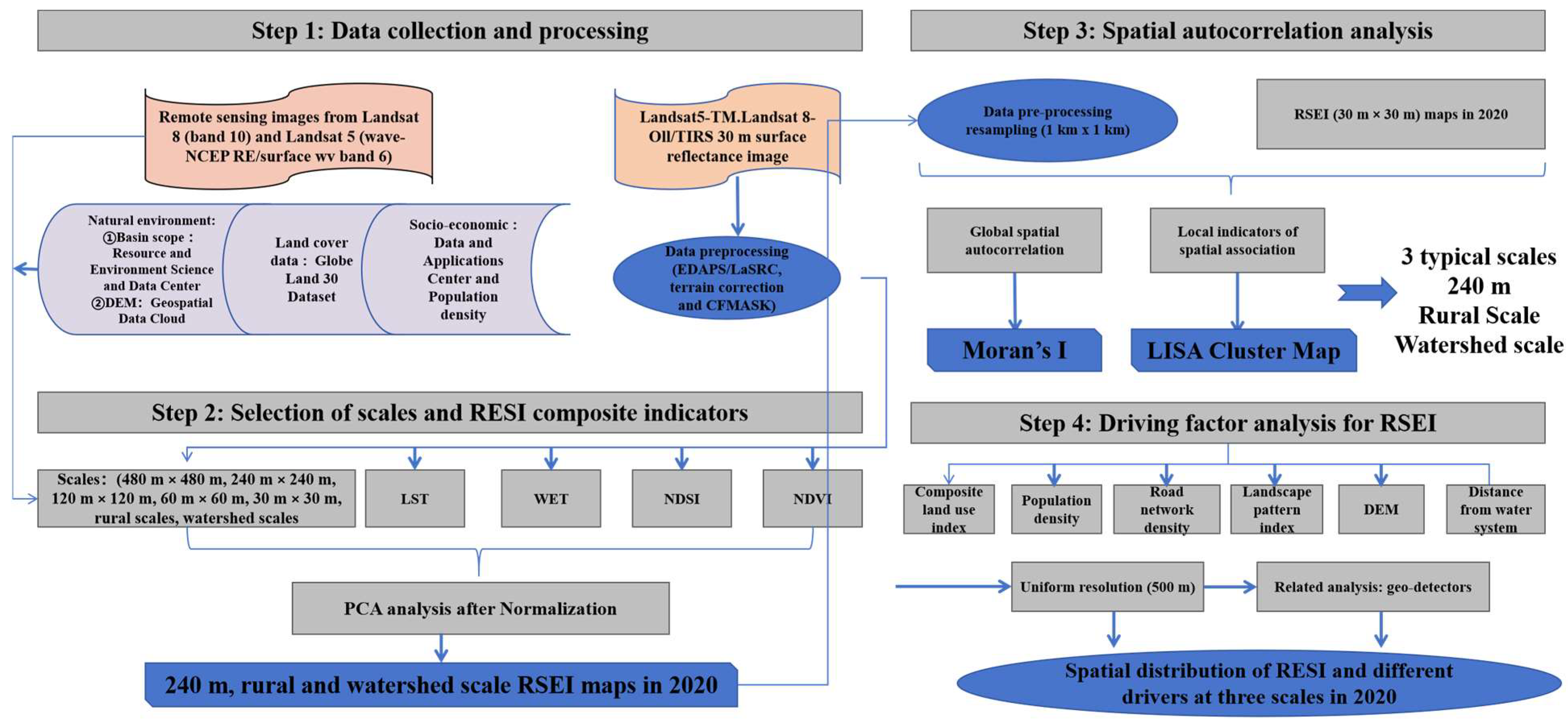
This study addressed the prevailing limitations of singularity and staticity inherent in the selection of evaluation units within RSEI investigations. Leveraging ArcGIS 10.3 grid sampling and magnitude transformation techniques, we systematically delineated a comprehensive framework comprising three distinctive categories of evaluation units, spanning a total of seven hierarchical levels. These units encompassed a range of isotropic scales (480 m × 480 m, 240 m × 240 m, 120 m × 120 m, 60 m × 60 m, and 30 m × 30 m). The selection of sample unit magnitudes within this range, spanning from 30 m to 480 m, is primarily influenced by data resolution parameters and the typical area dimensions of township administrative units within the Huashan Creek watershed.

Leveraging this diversified array of assessment units, we conducted a multifaceted assessment of RSEI within the Huashan Creek watershed. This holistic approach enabled us to conduct a comparative analysis of the spatial distribution of RSEI, discerning variations in heterogeneity across different scales within the study region. Additionally, this analysis unveiled the distinctive attributes characterizing the responsiveness of RSEI to alterations in spatial scales, shedding light on the underlying mechanisms influencing RSEI within the Huashan Creek watershed. By adopting this multifaceted approach, we aimed to mitigate against potential errors arising from a singular scale-centric perspective and ameliorate the issue of inadequately addressing spatial heterogeneity in the subjective delineation of evaluation units. See Figure 2 below for details.

2.2.2. RSEI

RSEI is a recently introduced comprehensive ecological assessment tool tailored to examine ecological conditions exclusively through remote sensing techniques [20]. RSEI comprises four distinct metrics, namely greenness, humidity, dryness, and heat (see

Table 2. Formulas and explanations for the four eco-quality indicators WET, NDVI, NDSI, and LST.

Index	Formula	Explanation
WET	β1Bblue + β2Bgreen + β3Bred + β4Bnir + β5Bswir1 + β6Bswir2	Bblue, Bgreen, Bred, Bnir, Bswir1, Bswir2represent the blue (0.45–0.51 µm), green (0.53–0.59 µm), red (0.64–0.67 µm), near-infrared (0.85–0.88 µm), short-wave infrared 1 (1.57–1.65 µm) and short-wave infrared 2 (2.11–2.29 µm) bands of Landsat 5 TM and Landsat 8 OLI/TIRS, respectively. βi is the corresponding band parameter [35,36];
NDVI	(Bnir − Bred)/(Bnir + Bred)
NDSI	(SI + IBI)/2	SI and IBI represent soil index and building index respectively [37];
LST	K1/ln(K1/D(t) + 1)	K1 and D(t) represent Planck’s constant and the radiative luminosity of a blackbody [38];

), each of which plays a critical role in ecological quality and can be directly perceived by human observers [35,36,37,38]. These metrics are derived from remote-sensing data, thereby ensuring a unified data source and minimizing the potential for errors stemming from disparate data sources. Prior research has substantiated the consistency, reliability, interpretability, and scalability of RSEI across diverse spatial and temporal scales [20]. Consequently, the computation of these metrics serves as a valuable tool for assessing ecological status based on readily available remote sensing data, often with minimal human intervention [39]. The formulas and significance of these indicators are presented in Figure S1.

In the initial step of the analysis, Landsat 8 satellite imagery underwent preprocessing involving removing clouds and identifying water bodies, accomplished through the GEE Platform. Concurrently, the four ecological indicators were subjected to wavelet transformation to derive normalized proxies. Ultimately, RSEI was obtained through PCA, which synthesized the contributions of each component. This comprehensive evaluation function ascertains the weighting of individual principal components, reflecting the proportion of information contributed by each component relative to the total information contained in the original dataset. This approach effectively mitigates the pitfalls associated with arbitrary weighting assignments and circumvents the impact of correlations among indicators, leading to a rational and objective determination of weights.

Moreover, the load weight of Principal Component 1 (PC1), as extracted from each indicator in the database through PCA, indicates significant changes. This method dispels the subjectivity inherent in conventional weighting approaches, yielding results that objectively, reliably, and expeditiously monitor and appraise the quality of the regional ecological environment. The functional expression of RSEI can be formulated as follows [40]:

$$\mathrm{R}\mathrm{S}\mathrm{E}\mathrm{I}={\mathrm{P}\mathrm{C}}_1\left[f\right(NDVI, \mathrm{Wet}, \mathrm{L}\mathrm{S}\mathrm{T}, NDSI\left)\right]$$

(1)

The applicable range of RSEI is [0,1] [33]. The proximity of the RSEI value to 1 signifies a high level of environmental quality. Within the context of this research, a comprehensive classification of the RSEI was conducted to gain deep insights into the spatial distribution patterns associated with remote sensing of ecological and environmental quality within the Huashan Creek watershed. This classification framework enables a quantitative and visually informative analysis [11]. To clarify, the RSEI of the Huashan Creek watershed was classified into 5 distinct grades at 0.2 isometric intervals, namely, “poor” (0–0.2), “fair” (0.2–0.4), “moderate” (0.4–0.6), “good” (0.6–0.8), and “excellent” (0.8–1) [23,33].

2.2.3. Characterization of RSEI

In the context of our investigation, PCA showed that the cumulative variance explained by PCA1 and PC2 accounted for 65.84% and 91.21% of the total variance, respectively. Deconstructing the contributions of the four constituent indicators within PC1, it was observed that the Green Index (NDVI) and the Wetness Index (WET) made positive contributions, while the Dryness Index (NDBSI) and the High-Temperature Index exhibited negative influences [41]. These findings affirm that enhanced greenness and wetness favorably impact ecosystem integrity, whereas increased dryness and elevated temperatures exert detrimental effects, aligning with real-world observations [37]. Conversely, the interpretation of positive and negative signals within the other principal components (PC2, PC3, and PC4) proved to be volatile and challenging to ascribe to ecological phenomena [33]. Given that PC1 encapsulates the majority of pertinent features and that the loadings of each indicator on the first principal component were uniformly distributed, the utilization of information extracted from PC1 for the characterization of RSEI in our study is a logical and sound approach.

2.2.4. Spatial Autocorrelation Analyses

The primary objective of Exploratory Spatial Data Analysis (ESDA) is to unveil the spatial configurations and associations among geographical entities, wherein geospatial location and arrangement play pivotal roles in determining the correlation among attribute values of these entities. ESDA elucidates geographical phenomena spatial distribution patterns and traits by employing diverse statistical metrics and analytical tools, including spatial autocorrelation, aggregation, and discrete indicators. Consequently, exploratory spatial statistics serve as a means to identify and investigate the clustering distribution pattern, spatial heterogeneity, and the presence or absence of spatial spillover effects within the realm of RSEI.

(1)

Global spatial autocorrelation (Global Moran’s I: MI)

The MI index measures the overall extent of global autocorrelation, encompassing the degree of spatial correlation heterogeneity and the differentiation in the distribution of RSEI. The vector formula for calculating Moran’s Index is presented below [3]:

$$\mathrm{M}\mathrm{I}=\frac{n}{\sum _i\sum _j{G}_{ij}}\mathrm{\ast }\frac{\sum _i\sum _j{G}_{ij}(x_i-\overline{x})(x_j-\overline{x})}{{\sum _i(x_i-\overline{x})}^2},$$

(2)

In this equation, MI denotes the global index, n is the total number of grid cells; Gij signifies the (i, j) element of the spatial weight matrix G (based on the variable K nearest neighbors, K = 4), following the principles of the first law of geography and inverse distance weighting. The values x_i and x_j correspond to the RSEI values of samples i and j, respectively, with $\overline{x}$ denoting the average RSEI values across the study area. MI is normalized by the spatial weight matrix G, yielding values within the range of [–1,1]. Regarding confidence levels, positive MI values indicate spatial clustering of RSEI in the province, with varying degrees of similarity and typicality. A close proximity to +1 signifies a positively correlated, significant clustering pattern, while a distant proximity from +1 implies a substantial divergence in atypical clustering, denoting a significant negative correlation with dispersion. Notably, MI values approximating or equal to zero signify a spatial distribution characterized by randomness, with no discernible correlation [42]. Additionally, the significance of the MI index was assessed using the Z-Score standardized statistic [42]:

$$\mathrm{Z}=\frac{MI-E\left(MI\right)}{SD\left(MI\right)},$$

(3)

where E(I) and SD(I) represent the theoretical mean and standardized variance, respectively, and MI signifies the global index. Specifically, when MI > 0 and Z-Score > 1.96, a considerable value indicates a vital and significant spatial positive correlation; conversely, a small value indicates a strong negative correlation and significant spatial variability [43].

(2)

Local spatial autocorrelation (Local Moran’s I: LI)

The RSEI MI solely captures the collective degree of divergence apparent within the broad spatial distribution of its density: it fails to elucidate localized disparities or pinpoint areas of concentration, as previously noted [44]. While LI is the decomposition of MI, the combination of LISA (local spatial association index to measure the level of significance) and the Moran scatterplot can reveal the scale or intensity of RSEI at the local, regional scale and its spatial autocorrelation with its neighboring places and its degree of significance. The formula for the LI is as follows [45]:

$${\mathrm{L}\mathrm{I}}_i={\mathrm{Z}}_i\mathrm{\ast }{\sum }_{j=1}^n{G}_{ij} \ast {\mathrm{Z}}_j,$$

(4)

$${\mathrm{Z}}_i=\frac{x_i-\overline{x}}{S^2},$$

(5)

$${\mathrm{Z}}_j=(x_j-\overline{x}),$$

(6)

where S² is the discrete variance of province i; Z_i and Z_j are the standardized mean values of RSEI for grids i and j, respectively, and the other variables have the same meanings as in Equation (2).

The Moran scatterplot form, which describes the correlation between variable A_i and its spatial lag vector B_(Ai), is dissected into distinct quadrants and categorized into five typologies [46], namely: random distribution of the origin (non-significant), clustering of high values (H–H type), low values surrounded by high values (L–H type), clustering of low values (L–L type), and high values surrounded by low values (H–L type). Among these values, under the given confidence level, if LI_i significantly > 0 and Z_i > 0, grid i is in the H–H quadrant; if LI_i significantly > 0 and Z_i < 0, grid i is located in the L–H quadrant; if LI_i significantly < 0 and Z_i > 0, grid i is located in the H–L quadrant; if LI_i significantly < 0 and Z_i < 0, grid i is located in the L–L quadrant [46].

2.2.5. Driver Analysis

(1)

Driver selection

The dynamics of RSEI are subject to a multifaceted interplay of factors encompassing natural attributes, land utilization, and socio-economic influences [47,48]. In this complex framework, natural determinants are paramount over extended time scales. Therefore, our investigation primarily highlights the pivotal role of specific natural elements affecting ecological traits within the focal area, which serves as the primary area for honeydew production. Among these salient natural determinants are elevation, which embodies considerations related to terrain, and proximity to water bodies, reflecting the importance of water sources.

Altitude significantly modulates the illumination, thermal conditions, hydrologic parameters, and nutrient status within the study domain, thus exerting a dominant influence on the distribution patterns of the landscape [49]. Simultaneously, rivers function as vital hydrologic conduits, attracting and reshaping nearby distributions of biodiversity, human activities, and ecosystem services, thus exerting a notable influence on the ecological milieu [50,51].

On the other hand, anthropogenic forces exert immediate and pronounced impacts at short temporal scales, ultimately directing the trajectory of local ecosystems in the long term. This study relies on indicators such as patterns of land use, socioeconomic parameters, and the spatial configuration of the landscape to gauge anthropogenic disturbance [14,52,53,54,55]. Among these indicators, changes in land use—manifested through shifts in structure, composition, and management practices—exert a pivotal influence on the functional and spatial balance of RSEI [56,57].

Socioeconomic factors such as the density of the population (an underlying determinant of human activities) and gross domestic product (GDP; acting as a visual gauge of ecosystem service value influenced by anthropogenic actions), tend to precipitate alterations in patterns of RSEI depletion as well as the quantity and quality of ecological amenities. This displacement results from social policies and developmental processes, further exacerbating the disruption of RSEI [58,59,60]. On the other hand, alterations in the spatial configuration of landscapes give rise to specific and discernable consequences by influencing the composition, structure, and ecological processes of ecosystems [61], thus molding RSEI [62,63].

In this study, we select indicators of landscape patterns designed to characterize landscape heterogeneity and levels of fragmentation, with the detailed meaning of these indicators elucidated in Figure S1. Therefore, a composite index consisting of land-use extent (La), population density (Pop), road distance (Dis_road), aggregation index (AI), maximum patch index (LPI), patch density (PD), Shannon’s diversity index (SHDI), distance from water (Dis_water), and elevation (DEM) is adopted, while its components serve as independent variables driving the factors in the RSEI model.

All data are normalized to a uniform spatial resolution of 500 m prior to analysis. In order to mitigate issues arising from collinearity between factors, we perform a correlation analysis and principal components analysis and select relevant scales (at the basin level and village level, covering an area of 240 km × 240 km) in order to ensure robust findings that are not affected by covariance between factors.

(2)

GWR

GWR is a valuable extension to the technique of local linear regression, designed to characterize spatially varying relationships within a given geographic region. This approach results in a regression model that elucidates local associations in discrete locations within a study area, effectively capturing localized spatial relationships and the inherent heterogeneity of variables. Finally, it should be noted that GWR has the distinct advantage of accounting for spatial dependence as well as variability within data, which is a departure from conventional global parameter estimation [3].

Another distinguishing feature of GWR is the inclusion of a weighting function, as it minimizes sample redundancy compared to traditional least squares methods, thereby increasing the accuracy of regression results and allowing spatially non-stationary relationships to be examined simultaneously [64,65]. The calculation model of GWR is

$${\mathrm{y}}_i={\beta }_0(u_i, v_i)+{\sum }_k^m{\beta }_k(u_i, v_i)\ast x_{ik}+{ϵ}_i$$

(7)

where y_i represents the dependent variable’s value at position i, k stands for the total number of grid cells, x_ik (k = 1, 2,..., m) signifies the value of the kth independent variable at point i, while (u_i, v_i) denotes the spatial coordinate of sampling point i. Furthermore, β₀ (u_i, v_i) corresponds to the intercept term of sample i, and β_k (u_i, v_i) embodies the regression coefficient for the k-th independent variable, x_ik, at sampling point i. This coefficient is a function of geographic location, ascertained through a weighted function method in the estimation process, and ϵ_i is the error term.

The accuracy of the GWR model is highly dependent on the choice of kernel function and bandwidth. We adopt the AIC method to determine the optimal bandwidth in this study given the ability of AIC to address accuracy quickly and efficiently. It is imperative to point out that a low AIC value in the model corresponds to a superior fit to the observed data, which indicates superior performance [66]. The degree to which various factors influence RSEI diverges across different spatial scales. Therefore, we use RSEI as a dependent variable and each influencing factor as an independent variable by building GWR models on three representative scales, which were selected based on the similarities and differences observed through spatial clustering, the availability and precision of the driving factors, the specificity of the administrative villages, the natural characteristics of the watershed, and the economy of the overall effort. The regression coefficients from these GWR models offer insights into the magnitude of influence exerted by the influencing factors on RSEI.

3. Result

3.1. Patterns of Spatial Differentiation in Ecosystem Quality at Multiple Scales

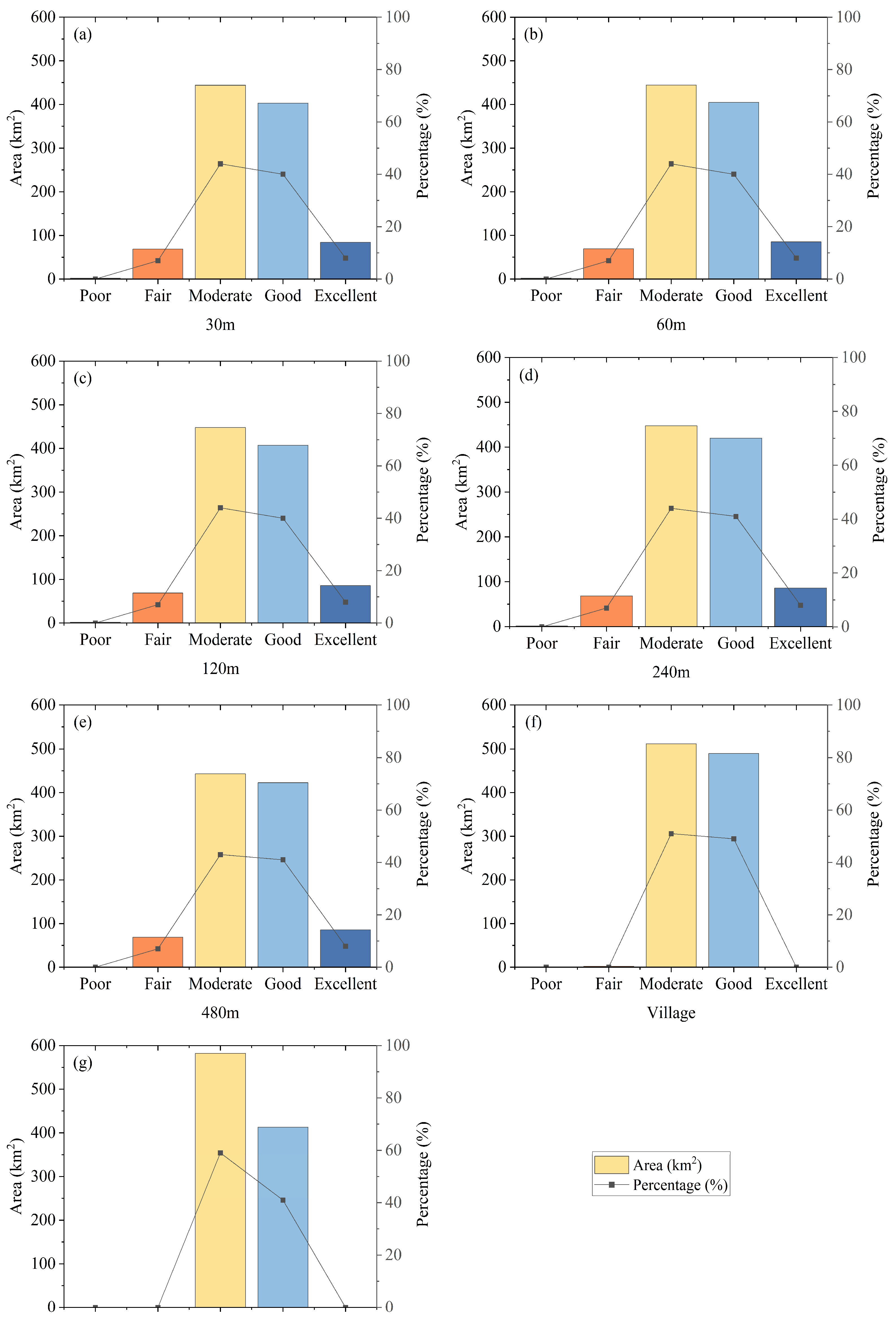
In order to elucidate the characteristics of ecological quality responses within the Huashan Creek catchment in relation to variations in spatial scale, we meticulously examine RSEI values across three separate scale units encompassing seven gradations in total. Correspondingly, we undertake a comprehensive analysis of the magnitude and inherent trends within these values. Figure 3 reveals distinctive spatial patterns in the distribution of RSEI across a variety of scales while retaining overall similarity. It should be noted that across scales, the predominant proportion of the surface exhibits a state of moderate RSEI, with favorable conditions seen in the eastern and western regions, juxtaposed with poorer quality conditions in the central region. As the scale decreases from 480 km to 60 km, the spatial granularity of the RSEI information within the grid cell types becomes finer, with relatively marginal differences exhibiting some degree of similarity. Regions characterized by excellent and good RSEI are scattered in the extreme east and west of the study area, respectively, creating a spot-like pattern.

The moderate RSEI region assumes a pentagram-like shape that is roughly positioned in the center of the region although areas showing poor RSEI concentrations are notably located in the north–central part of the study area, mainly at sub-rural scales, with sporadic occurrences in the north-western and south-central areas. At the rural and catchment scale, the distribution of RSEI occurs predominantly within the central core and periphery, showcasing moderate to high-quality performance. The extreme low zones (0–0.2) lie in the central watershed, which is in the core area of Pinghe County. Furthermore, taking advantage of the increased resolution of the 240 m grid, this study conducts an assessment of ecological environment quality scores at this scale, classifying them into 5 separate grades based on the size of the area: excellent (41.1%), good (43.7%), moderate (8.4%), fair (6.7%), and poor (0.1%). The results in Figure 4 reveal that the quality of the ecological environment within the Huashan Creek watershed predominantly occupies the moderate rating category at 8.4%, which is indicative of an overall moderate ecological status. To summarize, the overall distribution pattern of RSEI, whether at the administrative village level (Figure 4f) or at the grid scale (Figure 4a–e), highlights a prevalence of moderate and good conditions in contrast to a concentration of poor conditions in the urban center.

The magnitude of moderate RSEI coverage at the catchment scale (Figure 4g) exceeds that at the administrative village scale, with a noted concentration in the west–central part of the study area. Furthermore, the grid-scale delineates fine-scale areas with inferior RSEI distribution.

3.2. Spatially Dependent Characterization of Ecosystem Quality at Multiple Scales

3.2.1. Global Spatial Correlation Multi-Scale Spatial Response Characteristics of Remotely Sensed Ecological Quality

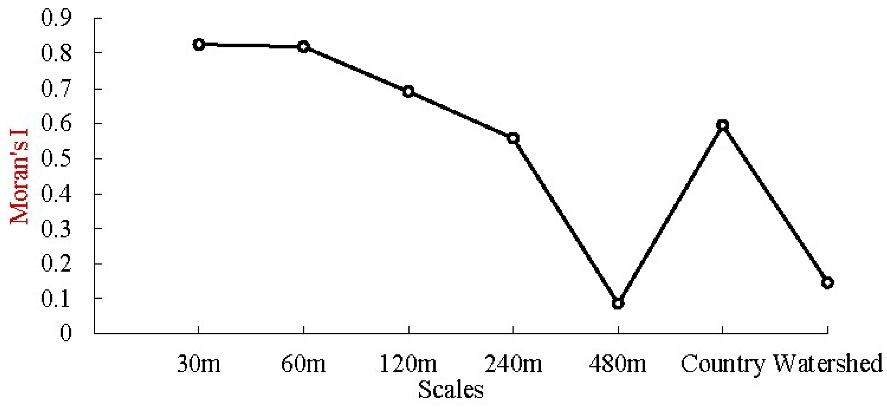
To analyze the spatial distribution differences of RSEI at three types of seven scales, this study describes the equilibrium pattern of RSEI using statistical parameters. Therefore, global indices of spatial autocorrelation derived from the Spatial Data Exploration and Analysis Methodology (SDEAM) are used as described in Equation (3). As illustrated in Figure 5, Moran’s I values for RSEI, computed at seven different scales over the course of 2020, showed a fluctuating pattern described as “increasing–decreasing–increasing” as the scale was decreased, revealing the presence of two scales characterized by indices of dissimilar spatial autocorrelation.

The overall pattern of fluctuations with respect to scale reduction follows a “bottom-up” pattern, indicating the existence of two scale cutoffs at the 480 km × 480 km scale (the lower limit) and the village scale (the steepest). Note that the transition from a grid scale of 30 m to 240 m results in a gradual decrease in the Moran I value, accompanied by minimal variations in its amplitude, which remained persistently greater than 0.6, indicative of a conspicuous spatial clustering. Then when the scale reached 140 m, the Moran I value showed a steep decline to 0.1 followed by a rapid rise to 0.6 at the village scale and finally decreasing to approximately 0.15 at the basin scale.

Overall, global Moran’s I values for RSEIs at the various scales consistently exceeded zero, with p values mostly below 0.001, with the Z-Score clearly exceeding 1.96, which clearly means the prevalence of highly significant positive spatial clustering in the spatial distribution of RSEIs across the seven separate scales of varying magnitudes. However, it is pertinent to note that the positive correlation features of agglomeration within the same grid scale type and across different scale types (grid, village, and watershed) manifest discernible differences.

In particular, when comparing the eigenvalues of the 5-level RSEI scale within grid scale types, there is a gradual increase in the overall Moran’s I value from 0.086 for the 480 m × 480 m case to 0.825 for the 30 km × 30 km case, with the former approaching minimum values near 0 and the latter approaching unity. Correspondingly, the Z-Score displays a rising trajectory as the range of scales decreases (ranging from 8 to 3379). This progression accentuates the significance and strength of the clustering of positive correlations within the RSEI at the grid scale, which becomes pronounced as the scale decreases. In addition, there is a remarkable jump in the Moran’s I value during the transition from 480 m × 480 m to 240 m × 240 m, while subsequent shifts between the remaining scales experience a change of roughly an order of magnitude, albeit with Moran’s I value dropping below 0.69 beyond 120 m × 120 m, indicative of decreasing significance in the clustering of positive spatial correlations.

Additionally, when contrasting village and watershed scale-type 2 scales, the global Moran’s I value for the former RSEI (0.595) substantially exceeds that of the latter (0.146), while the Z-Score exhibits a 13-fold increase (14.319 > 1.426). This divergence highlights the increased and statistically significant clustering of positive correlations evident at the village level. In addition, compared to the grid scale, the RSEI at the village scale displays similar Moran’s I values and Z-Scores to those observed at 240 m × 240 m, while the largest catchment scale stands out as unique, characterized by a Z-Score of less than 1.96, signifying clustering by weakly significant spatial correlation of RSEI.

With a Moran’s I value of 0.146, the watershed scale demonstrates a lack of statistically significant spatial clustering across cells, diverging from the pattern observed in the other assessments. As a result, it is discernible that within assessment cells of the same grid type, at microscopic scales of assessment, high Moran’s I values correspond to a great degree of spatial clustering in RSEI. In contrast, spatial clustering at the macroscopic catchment scale, similar to the case of 480 m × 480 m, lacks statistical significance. On the other hand, the mesoscopic scale of the village, analogous to the case of 240 m × 240 m, exerts a noteworthy influence on the spatial clustering of RSEI. Thus, the next section will focus on characterizing and analytically exploring the spatial distribution of RSEI at the microscale of 240 m × 240 m, at the meso-village scale, and at the macroscale of the watershed.

3.2.2. Local Spatial Correlation Multi-Scale Spatial Response Characteristics of Remotely Sensed Ecological Quality

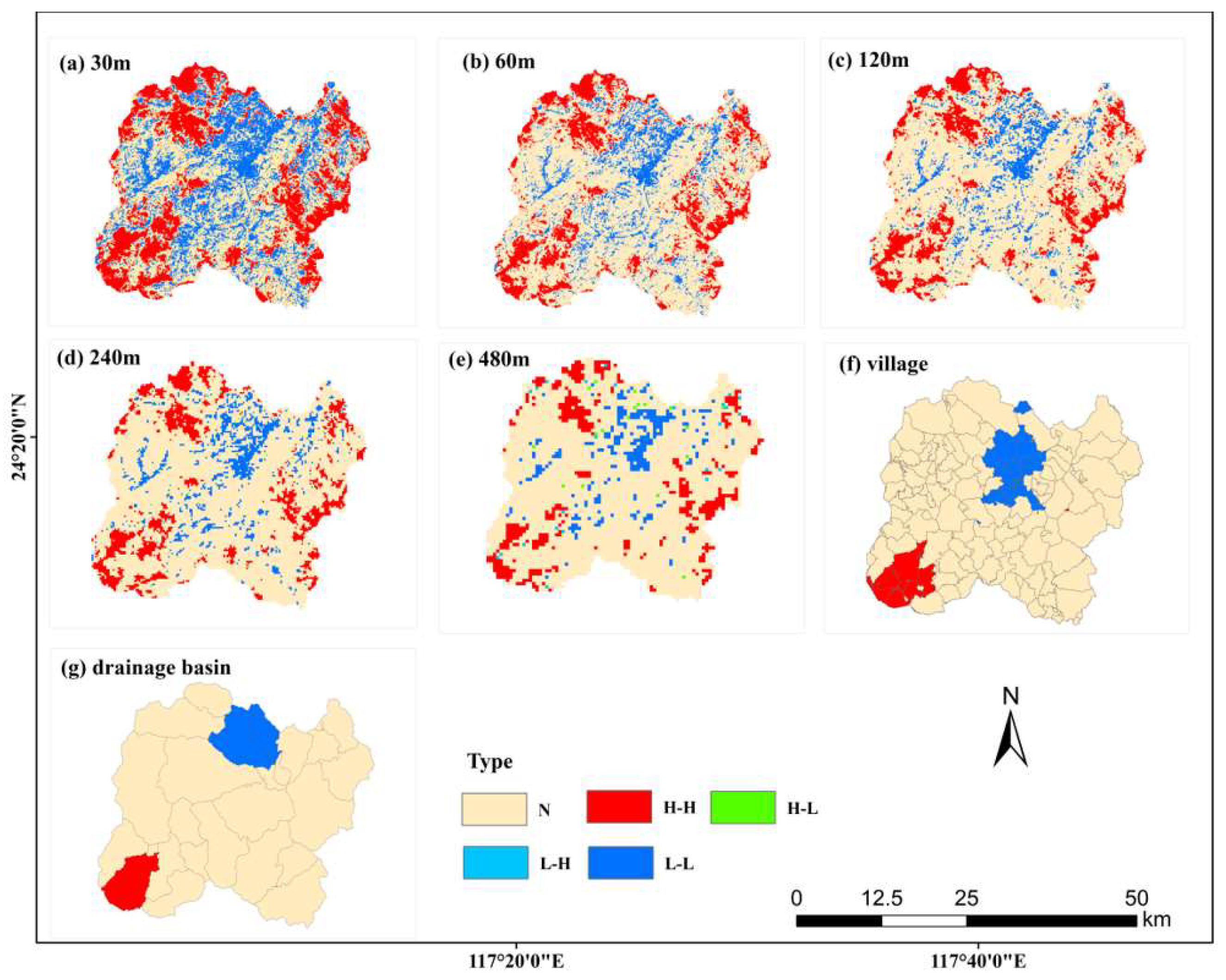
To further elucidate the local spatial autocorrelation and multiscale response characteristics of RSEI, this study employed a cross-scale assessment approach. In particular, the 240 m × 240 m grid scales, village administrative districts, and catchment scales exhibiting similar Moran’s I values are carefully chosen. The indices of local spatial autocorrelation derived from Equation (4) were then used to assess and analyze heterogeneity in the spatial correlation of RSEI across the study region as it experienced changes in the scales of the geographical unit types. Finally, it should be noted that there were both shared patterns as well as significant disparities in the local spatial differences in RSEI observed across varying scales.

As illustrated in Figure 6, except at the meso-village and macro-catchment scales, the spatial clustering pattern of RSEI at the grid scales was characterized by a non-random spatial distribution, while the non-significant regions increased in extent as the scales expanded. In addition, areas characterized as L–L and H–H types showed variation between scales. It is interesting to note that L–L and H–H regions consistently covered larger areas than those of the H–L type, and no regions exhibited the L–H type. Specifically, at the macro watershed scale, a multi-region spread displayed a combination of southwestern H–H and northern L–L types.

Similar distribution patterns were observed at a range of scales. On a meso-village scale, H–H continuous villages were prominent in the north–central region. At the 480 m × 480 m scale, there were few H–L types in the north–central region, with scattered H–H types in the SE and NW regions. At the 240 m × 240 m scale, there was a scattered H–L distribution, with a gradual concentration of H–H types in both the SE and NW. At the 120 km × 120 km scale, the H–L pattern was absent, with the central L–L pattern becoming continuous and the H–H pattern notably present in the NW, SW, and eastern parts of the country. At the 60 m × 60 m scale, an alternating pattern of H–H and L–L was observed in the east, center, and west. The alternating pattern between H–H and L–L was most distinct at the fine scale of 30 m × 30 m, especially in the upper, middle, and lower regions of the west. The H–H type was mainly located in the mountainous and vegetation-rich areas of the east and west, while the L–L type was prevalent in the central plains.

3.3. Response and Difference Analysis of Multiscale Drivers of Remotely Sensed Ecological Quality

A 240 m × 240 m grid was chosen for the identification of extraction points, informed by the ability of the grid to effectively mitigate outcome bias arising from covariance effects between factors as determined by correlation analysis and principal component analysis. A total of 11,141 sample points were then identified, each associated with specific driver values. Through an extensive filtering process employing correlation analysis, five independent variables were identified as suitable drivers, namely, distance from road (Dis_Road), population density (POP), density of patches (PD), distance from a water body (Dis_Water), and elevation (DEM). We then meticulously evaluated the impact of these variables on the RSEI dependent variable through GWR, which was conducted at multiple spatial scales. In order to provide deep insights into the factors that influence the local spatial distribution of RSEI, 3 separate geospatial cell scales: micro (240 m × 240 m), meso (village administrative district), and macro (watershed)-based were selected on the basis of their similarity in Moran’s I values. We then used the local GWR spatial coefficients derived from Equation (5) in order to dissect the variations in the effects of these five drivers across these diverse scales of geospatial cells.

3.3.1. Local Spatial Correlation: Multi-Scale Spatial Response Characteristics of Remotely Sensed Ecological Quality

Overall, the GWR results revealed a corrected R² of 0.42 and a condition number that was less than 0. These findings reflect the robustness of the model, which successfully withstood rigorous evaluations for multiple covariance considerations. The corrected R² surpasses the threshold of 0.6, indicating a relatively strong model fit. The regression coefficients within the GWR model provided insights into the individual indicators’ respective impacts on RSEI. We conducted a comparative assessment of these regression coefficients, focusing on the primary driving variables for RSEI within the Huashan Creek catchment at various spatial scales (i.e., watershed, village, and 240 m × 240 m) (see Figure 7). The driving variables for RSEI were observed to have positive influences at all three scales, with values greater than 0 indicating substantial positive effects. Among these, the socioeconomic variable POP displayed the most significant influence, consistently exceeding 0.7.

In addition to POP, the variables DEM and PD demonstrated noteworthy influences on RSEI. However, disparities emerged when comparing the magnitudes of these influences across different spatial scales. Notably, Dis_Road and POP maintained consistent coefficients across watershed scales, with approximate values of 0.4 and 0.8, respectively. Conversely, Dis_Water had the least impact at the village scale, registering a coefficient of 0.2 while displaying intermediate effects at other scales (0.5). In contrast, DEM exhibited its highest influence at the village scale (0.7) and intermediate impacts at other scales (0.5).

3.3.2. Analysis of Spatial Differences in Multi-Scale Remote Sensing Ecosystem Quality Drivers Based on GWR

Figure S1 depicts the spatial distribution of the five drivers, highlighting significant spatial variability in the relationship between RSEI and these factors, contingent on the analysis scale. Given this spatial layout, we categorized the regression coefficients into five distinct levels of intensity: 0 to 0.2 (low), 0.2 to 0.4 (low), 0.4 to 0.6 (medium), 0.6 to 0.8 (high), and 0.8 to 1 (high). In the same scale, specifically at the micro-grid level of 240 m × 240 m, DEM exhibited a systematic distribution of coefficient classes, with a concentration of coefficients ranging from moderate to high intensity extending from the central area of low-intensity coefficients to the periphery.

Approximately two-thirds of the area was dominated by moderate and high-intensity classes, with river valleys, characterized by lower topography, making a smaller contribution to RSEI at the grid scale. POP displayed four classes of coefficients above the low-intensity range, with the high and medium intensities being widespread and the high intensity contiguous. Moderate, weak, and strong intensities were mostly clustered in the southwestern corner of the study area. Both Dis_Road and Dis_Water methods covered all coefficient classes. The distribution of Dis_Road appeared patchy, primarily in the north–central to south–central areas, with the moderate intensity area predominating. On the other hand, Dis_Water exhibited an alternating cluster-band pattern, with the moderate intensity area being the most extensive and the lower intensity low appearing as scattered spots.

The high-intensity area was primarily located to the northwest and south. PD extended across all gradient levels, with coefficients increasing toward the southeast in the northwest corner. In the rest of the region, the high-intensity center retreated outward, with the moderate area mostly in the southwest-to-eastern margins. At the rural mesocosmic scale, DEM exhibited three high-intensity coefficient classes, covering most of the region in an east-west and south-north direction, while the moderate-intensity class dotted the edges from east to west. On this scale, POP had four coefficients lower than the high intensity, with the low-intensity class spanning the region, and the moderate to high-intensity classes primarily found in the southwest corner.

Dis_Road, Dis_Water, and PD showed the full range of classes. Dis_Road featured a substantial area of high intensity that was contiguous to the west, with intensity gradually increasing from south to the northeast. Dis_Water displayed a gradual increase in intensity from the southwest to the northeast, with an area of high intensity to the northeast. PD showed a distinct increase in intensity from north to south, with a notable presence of average intensity in the northeast corner. At the macro watershed scale, each factor consisted of five classes and displayed a more even distribution. DEM, Dis_Water, and PD showed a gradual increase from the west to the east, with Dis_Water showing the most pronounced increase. DEM showed a high-intensity region in the southeast-northeast corner, while PD displayed a high-intensity area in the southeast-northeast corner. On the other hand, POP demonstrated an increase in intensity from the south to the north, whereas Dis_Road showed an increasing distribution from east to west.

With respect to the impact of the same driver at different spatial scales, the influence of DEM on RSEI increased as the scale transitioned from the microgrid scale to the meso-grid scale, subsequently exhibiting a slight attenuation at the macroscale of the watershed. The impact of POP on RSEI was most pronounced at the micro-scale and minimized at the meso scale, with relatively uniform contributions observed at the macro-catchment scale and within sub-catchments. The strength of the effects of Dis_Road and Dis_Water also intensified as the scale broadened, whereas the spatial distribution shifted from a pattern of dispersed clusters to a hierarchical east-west distribution. Of note, the range of PD’s high-intensity impacts steadily decreased with the increase in scale.

4. Discussion

4.1. RSEI Response to Spatial Scales

For the three scale categories, as the scale resolution increases from 60 m to the catchment scale, the response of the ecological environmental suitability scale at seven distinct levels primarily shifts in attributes related to RSEI, ranging from complex and detailed spatial distributions to more straightforward and clearer models. However, there is a risk that the perception of a shift might obscure critical information [28]. Notably, RSEI spatial correlation reaches its lowest point as the scale expands to 480 m. Moreover, at the village scale, the spatial distribution results diverge markedly from those at the earlier scale, with the disparity growing significantly at the catchment scale (see Figure 3).

The study area was examined using the same research methods and data. The spatial distribution characteristics exhibit distinct patterns due to variations in the scale of the assessment units. This behavior reveals significant variability between scale categories but limited variability within each category. This variability occurs because evaluations of differences in environmental quality are sensitive to changes in the size of the assessment units involved. Large units reflect the local composition of the landscape or specific terrestrial ecological subsystems. Furthermore, as the unit size increases, RSEI evaluations tend to minimize differences in landscape elements within the unit [28].

In summary, this study highlights the importance of conducting RSEI response analyses at various spatial scales. Reliance on single-scale assessments alone often fails to accurately assess regional ecological quality since it does not comprehensively represent the true state of an area and desired outcomes. Thus, employing RSEI to analyze responses at different spatial scales is advantageous. Such an approach can mitigate errors arising from single-scale divisions and address issues related to the incomplete consideration of spatial heterogeneity in the division of assessment units. The choice of scale, however, should reflect analytic goals, available information, and decision-making requirements [67].

In this study, the alteration of spatial scope yields distinct characteristics in the global autocorrelation spatial analysis of ecological quality and functional control across three scale levels: sample grid, administrative boundary, and watershed scales, all based on natural ecosystems. The Moran’s I value of the RSEI exhibits a fluctuating “decreasing-increasing-decreasing” pattern as the scale expands, revealing notable variations. In particular, as the scale of the grid increases, the information becomes less detailed, resulting in a gradual decrease in Moran’s I.

The most significant difference in Moran’s I value of RSEI was observed between the 240 m scale and the 480 m scale. This is because, at the 240 m scale, RSEI’s spatial performance is similar to that calculated in rural areas, resulting in a higher spatial autocorrelation of 0.6. This result is much higher than the spatial autocorrelation of 0.15 at the watershed cell scale and 0.1 at the 480 m grid sample scale. Therefore, the 240 m and rural scales are useful for identifying spatial differences in ecological quality within the Huashan Creek watershed as well as for further analysis. The central valley examined in this study, characterized by poor drainage, has a more significant influence than elevation alone, primarily due to population growth and socio-economic development. Original forested areas and water bodies were cleared for agriculture and construction, increasing the amount of land used for these purposes. The change led to the fragmentation of once-contiguous forests and the formation of only a few isolated forested patches and small lakes. The actions exacerbated fragmentation, affecting the RSEI of the watershed and contributing to the land’s unsuitability for honeydew cultivation. The western and eastern areas are closer to transportation routes that fragment the original forest cover and water bodies, resulting in areas that are at a greater distance from water bodies. However, the highly impacted area in the northwest corner may be used as a nature reserve, creating an ecological barrier that fosters biodiversity, raising the RSEI.

At the 480 m scale, spatial correlation is lowest because of its masking effect on finer ecological features, such as small lakes and vegetation. In the Huashan Creek watershed, where a significant portion of the land is used for honeydew production, the rural and the watershed scales are both appropriate for RSEI assessments. The approach is justified by the practicalities of collecting data and establishing ecological control models within administrative units, making it more feasible than utilizing larger watershed units spanning multiple regions. Administrative data at the village level offers greater accuracy for higher-level units and, when combined with grid-scale data, provides detailed support for village and catchment planning and protection efforts [68].

We utilized 240 m, rural, and watershed scales to assess RSEI within the district because we recognized the importance of natural catchment boundaries for the assessment of land use impacts and water quality change. Local autocorrelation spatial analysis was used to examine RSEI clustering. At larger scales, the finer grid scales fail to establish spatial correlation because they average high RSEI values across the eastern and western portions of the district.

Analysis using the 240 m, the village, and catchment scales revealed areas of excellent ecological quality (H–H), which are clustered in mountainous areas with dense vegetation cover, notably in the south-west. In contrast, poor ecological quality (L–L) areas are in the central–northern region, marked by low relief, degraded vegetation, urbanization, and high population densities. Mixed ecological quality areas are found in flat areas where urban and natural ecosystems co-exist. The central area, marked by low elevation and high population density, exhibits moderately poor ecological quality [23].

4.2. Response of RSEI Drivers to Spatial Scales

4.2.1. Key Drivers of RSEI

RSEI within the Huashan Creek watershed is influenced by various factors, including DEM, POP, Dis_Road, Dis_Water, and PD. However, the extent of these influences and their spatial distribution varies across scales and locations. Collectively, POP, DEM, and PD determine the magnitude and spatial pattern of RSEI at all scales, with POP having the most significant impact (approaching 0.8). Natural population growth and migration can result in urban expansion, reduced vegetative cover, and frequent changes in land use. Anthropogenic activity contributes to increased water use and elevated greenhouse gas emissions, affecting urban climate factors such as temperature, humidity, and aridity [69,70,71]. Elevation has a significant influence on factors such as rainfall distribution, temperature, radiation intensity, soil quality, plant ecology, growth, and overall ecological quality. It shapes human activities, including agriculture, industry, and transportation, with lower elevations generally experiencing a greater human impact, which increases the RSEI. Specifically, areas at lower elevations usually have higher population densities, road densities, patch densities, and distances to water bodies. Areas with these types of integrated landscapes are more susceptible to soil erosion and pollutant transport from upstream areas, which can reduce ecological quality [69]. The areas where DEM had the highest influence primarily consisted of those at lower elevations that were suitable for honeydew cultivation, where greenness, temperature, humidity, and desiccation had a significant influence. As Xiong et al. [33] indicate, ecological restoration or agro-industrial planning at the larger scale of the Minjiang River should first be done on steep north-facing slopes at low elevations. Shao et al. [72] also demonstrated that the combination of topographic superimposition of conditions such as humidity and greenness and anthropogenic activities is the key factor influencing the ecological quality of Qingdao city.

Regarding the other variables, there was significant spatial heterogeneity in the influencing factors in different regions and at different scales [73]. Li et al. [34] suggest that human activities contribute to the improvement of eco-environmental quality by reducing the degree of landscape fragmentation and the intensity of land use. Xiong et al. [33] indicate that the relationship between NDVI and topography is scale-dependent. Wu et al. [74] reveal that precipitation and land use are the main factors affecting the Sichuan-Yunnan Ecological Barrier Area, but they have different interpretations at different unit scales. Ling et al. [75] pointed out that vegetation, anthropogenic disturbances, and aridity index were the main factors influencing ecosystem services in the Manas River basin.

Furthermore, changes in landscape patterns, such as fragmentation, have implications for functions such as productivity, connectivity, climate regulation, and ecosystem health. Comparing key drivers at different scales, it is clear that proximity to roads and water bodies has a relatively similar impact on catchment scales, highlighting the rivers’ vital role as water conduits. At the village level, proximity to water bodies has a more substantial effect than road distance because of the importance of irrigation, which affects water quantity and quality [20]. The construction of government road networks in rural areas highlights the importance of road distances to the characterization of an ecological environment. The performance of the 240 m grid scale is similar to that of watershed scales. Overall, the quality of an ecological environment is shaped by natural factors and changes in land use. Therefore, at lower elevations, anthropogenic activities will outweigh the effects of elevation. The increase of cultivated land, transportation, and construction land exacerbates the fragmentation of existing landscape patches such as forests and water bodies, whereas the establishment of nature reserves restores the environmental characteristics. These impacts will inevitably alter the RSEI.

4.2.2. Driven Response of RSEI at Different Scales

At the microgrid scale, regions with smaller contributions to RSEI are clustered in the central lowlands. Areas with higher populations and diverse land-use patches extend outward from the central region, forming a “pentagram” pattern. This pattern arises because of the significant influence of human activity, especially in poorly drained areas. Although drainage is limited, the central valleys provide an environment conducive to development. The increase in population and economic development leads to the expansion of agriculture and construction in the core areas, fragmenting the landscape and affecting the measured ecological quality. The transformation of forests and aquatic ecosystems into cultivation land leads to the fragmentation of forests and small lakes, thereby negatively impacting the ecological quality of watersheds.

Furthermore, the proximity of transportation routes to the western and eastern regions, facilitated by external links, intensifies the reduction of forest cover and the fragmentation of water bodies [76]. Factors associated with dispersed clusters of water bodies at varying distances are observed, with many areas showing negligible impact due to water resource depletion caused by human activity. In contrast, specific high-impact regions in the northwest corner play a crucial role because water bodies function as ecological obstacles and biodiversity reserves. Villages at the meso-rural level were influenced by the composition of rural populations and the fragmentation of land, reducing local human disturbances by minimizing the impact of rural out-migration on RSEI at larger scales. Additionally, villages in environmentally sensitive areas, especially at higher elevations in the southwest, may have a substantial influence on RSEI. At this scale, natural factors such as elevation and water bodies dominate. The “Y”-shaped area in the northern and central regions, which is close to water bodies and roads, provides ample resources for honeydew production and attracts residents.

Unsustainable practices and chemical inputs can contaminate and harm biodiversity and ecosystems [77]. At the macro watershed scale, the five influencing factors show a more even spatial distribution because watershed analysis smooths the impact of subtle features such as slope, water masses, and patch density. As we move eastward into the Huashan Creek drainage basin, decreasing elevation and increasing water masses result in the fragmentation of patches, intensifying the combined effect of these factors. Significant differences can be observed in the northern region, which houses a central urbanized catchment area where anthropogenic disturbance is more pronounced. Conversely, the high-elevation, sparsely populated western region features minor human activity in vulnerable mountainous areas, particularly in less developed regions such as Xiazhai Town and Guoqiang Town. In more isolated regions, the expansion of roadways can lead to the depletion of resources, permanently damaging the natural environment.

Notably, the smaller and larger scales of POP influence have a more pronounced effect on the spatial distribution of RSEI. However, the spatial pattern of the influence of DEM is apparent at larger rural scales [33], indicating that the higher the elevation, the more pronounced the spatial spread of RSEI. When the grid size employed in the analysis is smaller than typical micro geomorphic unit sizes, the finding highlights the importance of regional landscape, population density, and patch fragmentation. In contrast, when the grid size employed in the analysis is larger than the mean grid size, this approach is more likely to identify the impact of broader topographic patterns, water masses, and the distribution of transport routes while potentially neglecting finer-scale subtleties [78,79]. Overall, conducting a multi-scale driver analysis is more beneficial to our understanding of the mechanisms driving RSEI, offering valuable information on selecting environmental motivators at various levels.

4.3. Selection of Scale

This study examines the spatial response patterns of RSEI at different scales, such as 30 m, 60 m, 120 m, 240 m, 480 m, rural, and watershed scales. Previous research has demonstrated that the Huashan Creek watershed, where human activities and natural elements affect each other, is subject to considerable ecological strain [80,81]. Significantly, the spatial patterns of RSEI exhibit incongruous regional disparities in scale and location. Although detailed micro-level research can provide exact information, a more thorough examination may be needed [82]. Although administrative village scales effectively provide information on overall distribution and they may help decision-makers in precise management based on administrative boundaries, they may need to identify micro-spatial intricacies to make better decisions. Huang et al. and other researchers note the need for deeper understanding when evaluating the Chengdu-Chongqing Urban Agglomeration on a larger scale, indicating it is common for assessments to fail to acknowledge the variations in small-scale landscape components and structures [67].

Consequently, depending solely on a single-scale evaluation provides an inadequate approach for identifying varied ecological characteristics, suggesting there is no universally applicable scale for comprehensive assessments. Instead, it is essential to employ global and local spatial autocorrelation to assess attribute values and spatial discrepancies among geographic units that are created while paying attention to the unique qualities of various sizes [83,84]. Figure 6 highlights the substantial influence of spatial clustering at the scale of the mesocosmic village, such as the 240 m × 240 m scale, exhibiting a relatively large Moran’s I of 0.6. This observation is important in both grid and administrative scale evaluations. The watershed-scale also demonstrates distinctive representativeness, with natural ecosystems delineating watershed boundaries, providing a more intuitive and scientifically sound basis for assessing land use and water quality change. It is worth noting that the Huashan River, a major tributary of the West Creek of the Jiulong River that is located in an area that engages primarily in honeydew production, has been the focus of significant local government efforts relating to economic development and environmental management [31].

By examining the similarities and differences in the observed spatial clustering, the availability and precision of the driving factors at different scales, the social specificity of the administrative areas, the overall typicality of the Huashan Creek Watershed, the variability of Moran’s I, and the economy and sustainability of the overall workload, the 240-metre grid, the villages, and the watershed scales were used as the criteria for assessment. Moran’s I at 240 m was found to be relatively high and close to 0.6 at the village scale (Figure 5), reflecting more information spatially than at the village scale. This comprehensive assessment methodology facilitates the examination of spatial discrepancies in geographical characteristics, topography, and administrative area size within the district. Additionally, the assessment approach supports the development of ecological management and compensation strategies, the extraction of accurate village-level data, and the production of individual watershed maps. Ultimately, this method can help researchers create an all-encompassing database containing both natural and socio-economic data. In summary, it is essential to ensure that the scale chosen for RSEI management policies is in line with analytical objectives, available information, and scale-related data, meeting stakeholders’ decision-making needs to achieve maximum relevance.

4.4. Policy Implications

Gaining insight into the elements contributing to disparities in ecological quality in the Huashan Creek watershed is critical for formulating plans to manage ecosystem operations and coordinate efforts to ensure ecological preservation and enhance economic activities suitable for local circumstances. Examining the factors influencing RSEI spatial differentiation using geographically weighted regression across different scales demonstrates that considering the collective impacts of human activities, natural elements, and landscape patterns significantly enhances our ability to identify RSEI spatial disparities. Landscape fragmentation can have a multitude of impacts on the ecological quality of the Huashan Creek watershed, influencing population dynamics, elevation, watershed water management, and honeydew production zones. These impacts can have cascading effects on the water, air, land, soils, and biological diversity of the environment.

The idea of ‘patches’ illustrates how land-use changes can drastically alter the ecological balance of a given area, which is frequently linked to the numerous honeydew gardens that constitute almost 60% of the Huashan Creek watershed. To ensure the successful management of ecological services, it is essential to implement specific strategies to minimize other human-caused disruptions and enhance the regional landscape structure and patterns, particularly considering the simultaneous impact of diverse landscape arrangements and activities associated with the thriving growth of the honeydew sector.

For instance, in high-altitude western mountainous regions characterized by intensive land development, efforts should reduce socio-economic activities while promoting environmentally friendly sectors such as sightseeing, eco-agriculture, and recreational demonstration facilities. Additionally, when expanding the honeydew industry, it is imperative to bolster ecological control and protection initiatives to prevent the exacerbation of problems such as soil erosion, forest cover reduction, water scarcity, and desertification. The optimization of regional landscape structures is particularly important because it enhances ecological security and diminishes the risk of compromising ecosystem functions due to the combined influences of elevation and human interference.

Enhancing ecological environmental quality requires optimizing activities based on landscape patterns in areas marked by intense human economic activities, such as the central plain zone within the area under study. This approach helps mitigate the potentially adverse effects of the interaction between anthropogenic interference factors and landscape pattern index factors on regional environmental quality, thereby preventing a decline in ecological environmental quality. It is essential to strictly adhere to arable land protection policies, which should be enforced in grain-producing regions to prevent arable land degradation and promote high-quality green development. During periods of population growth, urban expansion should adhere to well-defined boundaries between rural and urban areas. This approach can lead to efficient land use practices, restraining haphazard expansion and minimizing land resource wastage. Furthermore, the establishment of ecological corridors, green buffer zones, and ecological parks in and around central cities can enhance livability and support sustainable urban development.

4.5. Limitations and Prospects

In this study, we use human–land interaction theory and landscape ecology to develop a comprehensive framework consisting of two distinct approaches and three modes of operation. Our findings can be used to regulate the quality of the ecological environment within the Huashan Creek watershed. First, this analysis is conducted at the scale of township administrative units, where the Huashan Creek watershed could be effectively managed through two strategies: “change in land-use pattern and improve land-based ecosystem service function” and “adjust land-use structure and improve land ecosystem service function”. These strategies are implemented within the overarching framework of “synergizing regional economic development, protecting the ecological environment, and precisely alleviating poverty”.

In the context of “coordinated regional economic development, ecological, environmental protection, and precise poverty alleviation”, optimizing ecological environment quality is achieved through “changing the land use mode to improve the function of land ecosystem services” and “modifying the land use structure to optimize the allocation of ecological landscape resources”. This work was facilitated by a regulatory approach characterized by “precision, differentiation, and diversification”. Conducting comparative assessments across multiple administrative unit scales, specifically focusing on the Huashan Creek watershed, is crucial for future research. This will help determine the most suitable administrative unit scale that aligns with the distinctive attributes of the study area, facilitating further investigations. Exploring the feasibility of gathering information on specific drivers of change, especially for assessing long-term ecological quality developments in the research region, could be a promising approach for forecasting future changes.

It is essential that a more comprehensive range of independent variables is considered when making decisions, including economic regulation, ecological compensation, zoning adjustments, and regional monitoring. The impact of employing these elements needs to be assessed. Therefore, a thorough comprehension of their intricate connections with natural, socio-economic, land-use, and policy elements and their effects on ecological quality is needed. Because current ecological quality models may not fully capture the complexity of the regional ecosystem quality, it is crucial that more suitable and representative indicators are identified to aid the integration of a broader array of data sources to enhance the assessment of regional ecological quality [41].

This research provides a useful examination of how, across different areas and scales, specific drivers of change impact RSEI in the Huashan Creek watershed. The primary objective of this study is to establish a reliable and effective system for continuously assessing the ecological quality of a region. By exploring the elements that may influence changes in the ecological environment and delving deeply into how various elements shape ecological environmental quality, this research provides a foundation for implementing well-informed ecological protection and urban development strategies within the study area [85]. Empirical evidence has confirmed the effectiveness of remote sensing ecological indices in effectively depicting the ecological environment. Ongoing efforts to enhance correlation indices and understand the connections between these index factors are expanding the horizons of research [81,86].

5. Conclusions

Based on the environmental equilibrium matrix of the Huashan Creek watershed at three types and seven scales in 2020, this study constructed a regional environmental index (RSEI), revealed spatial response characteristics of the RSEI to different scales, and analyzed the key drivers of the RSEI. The results are as follows:

(1)

Global autocorrelation revealed that the size and area information associated with the RSEI gradually transitioned from a complex-detailed to a more intuitive and clearer pattern as the scale resolution decreased. The fusion analysis of 240 m unit, rural, and watershed scales can not only encompass the rich information on RSEI spatial differences but can also provide data support and a more intuitive scientific assessment of the impacts of land use and water quality changes;

(2)

Local autocorrelation showed that RSEI exhibits relatively apparent spatial aggregation characteristics at different scales. The RSEI of the Huashan Creek watershed in 2020 was generally moderate. Areas with poor RSEI were concentrated in the built-up areas and riparian zones of the towns and cities in the central plain area. In contrast, areas with higher RSEI were concentrated in the western mountains with greater vegetation cover;

(3)

Using PCA, we identified five key factors affecting RSEI: DEM, POP, Dis_Road, Dis_Water, and PD. Moreover, using GWR and controlling for confounding geographic factors, we found that human activities had a significant effect on environmental quality. The population was found to have a significant effect at all three scales. Elevation was significant at the administrative village level, while the patch landscape index significantly affected the grid and catchment scales. Complex interactions between natural features, land use, and socio-economic factors exacerbate the fragmentation of landscape patches, amplifying their effects on ecosystem quality in a non-linear manner. These complex interactions highlight the critical role of elevation, population, proximity to roads, and proximity to water bodies in shaping the ecological integrity of the region.

References

1. Venter, O.; Sanderson, E.W.; Magrach, A.; Allan, J.R.; Beher, J.; Jones, K.R.; Possingham, H.P.; Laurance, W.F.; Wood, P.; Fekete, B.M. Sixteen years of change in the global terrestrial human footprint and implications for biodiversity conservation. Nat. Commun. 2016, 7, 12558. [Google Scholar] [CrossRef] [PubMed]
2. Costanza, R.; d’Arge, R.; De Groot, R.; Farber, S.; Grasso, M.; Hannon, B.; Limburg, K.; Naeem, S.; O’neill, R.V.; Paruelo, J. The value of the world’s ecosystem services and natural capital. Nature 1997, 387, 253–260. [Google Scholar] [CrossRef]
3. Liu, Z.; Wu, R.; Chen, Y.; Fang, C.; Wang, S. Factors of ecosystem service values in a fast-developing region in China: Insights from the joint impacts of human activities and natural conditions. J. Clean. Prod. 2021, 297, 126588. [Google Scholar] [CrossRef]
4. McDonnell, M.J.; MacGregor-Fors, I. The ecological future of cities. Science 2016, 352, 936–938. [Google Scholar] [CrossRef] [PubMed]
5. Lin, J.; Huang, J.; Hadjikakou, M.; Huang, Y.; Li, K.; Bryan, B.A. Reframing water-related ecosystem services flows. Ecosyst. Serv. 2021, 50, 101306. [Google Scholar] [CrossRef]
6. Cai, J. Study on water environmental protection countermeasures of Huashan Stream in Pinghe County. Leather Manuf. Environ. Technol. 2021, 2, 18–20. [Google Scholar]
7. Huang, W.; Chen, G.; Hu, C. Real time regional soil erosion evaluation based on RS technique—Case study in Huashanxi Watershed, Fujian Province. Chin. J. Geol. Hazard Contr. 2003, 14, 118–120, 126. [Google Scholar]
8. Han, S. Optimal allocation of water resources in Pinghe County and its surrounding towns. Hydr. Sci. Technol. 2023, 1, 14–17. [Google Scholar]
9. Wen, X.; Lin, Z.; Tang, F. Remote sensing analysis of ecological change caused by construction of the new island city: Pingtan Comprehensive Experimental Zone, Fujian Province. J. Appl. Ecol. 2015, 26, 541–547. [Google Scholar]
10. Wang, G.Y.; Mang, S.; Cai, H.S.; Liu, S.R.; Zhang, Z.Q.; Wang, L.G.; Innes, J.L. Integrated watershed management: Evolution, development and emerging trends. J. For. Res. 2016, 27, 967–994. [Google Scholar] [CrossRef]
11. Song, H.M.; Xue, L. Dynamic monitoring and analysis of ecological environment in Weinan City, Northwest China based on RSEI model. J. Appl. Ecol. 2016, 27, 3913–3919. [Google Scholar]
12. Wu, Z.; Wang, M.; Chen, S.; Zou, D. Monitoring and evaluation of ecological environments spatio-temporal variation in mine based on RSEI a case of Yongding mine. Ecol. Sci. 2016, 35, 200. [Google Scholar]
13. Zhang, H.; Du, P.; Luo, J.; Li, E. Ecological change analysis of Nanjing city based on remote sensing ecological index. Geosp. Inf. 2017, 15, 58–62. [Google Scholar]
14. Xu, M.; Chen, C.; Deng, X. Systematic analysis of the coordination degree of China’s economy-ecological environment system and its influencing factor. Environ. Sci. Pollut. Res. 2019, 26, 29722–29735. [Google Scholar] [CrossRef] [PubMed]
15. Xiao, W.; Guo, J.; He, T.; Lei, K.; Deng, X. Assessing the ecological impacts of opencast coal mining in Qinghai-Tibet Plateau-a case study in Muli coal field, China. Ecol. Indic. 2023, 153, 110454. [Google Scholar] [CrossRef]
16. Sishodia, R.P.; Ray, R.L.; Singh, S.K. Applications of remote sensing in precision agriculture: A review. Remote Sens. 2020, 12, 3136. [Google Scholar] [CrossRef]
17. Wang, S.; Zhang, X.-X.; Zhu, T.; Yang, W.; Zhao, J. Assessment of ecological environment quality in the Changbai Mountain Nature Reserve based on remote sensing technology. Prog. Geogr. 2016, 35, 1269–1278. [Google Scholar]
18. Liu, C.; Wu, X.; Wang, L. Analysis on land ecological security change and affect factors using RS and GWR in the Danjiangkou Reservoir area, China. Appl. Geogr. 2019, 105, 1–14. [Google Scholar] [CrossRef]
19. Zhang, R.; Li, C.K.; Yao, S.; Li, W. Study on the change factors of construction land in Taiyuan by integrating geographic detector and geographically weighted regression. Bull. Surv. Mapp. 2022, 5, 106–109, 119. [Google Scholar]
20. Xu, H.; Wang, M.; Shi, T.; Guan, H.; Fang, C.; Lin, Z. Prediction of ecological effects of potential population and impervious surface increases using a remote sensing based ecological index (RSEI). Ecol. Indic. 2018, 93, 730–740. [Google Scholar] [CrossRef]
21. Gao, P.; Kasimu, A.; Zhao, Y.; Lin, B.; Chai, J.; Ruzi, T.; Zhao, H. Evaluation of the temporal and spatial changes of ecological quality in the Hami oasis based on RSEI. Sustainability 2020, 12, 7716. [Google Scholar] [CrossRef]
22. Hang, X.; Li, Y.; Luo, X.; Xu, M.; Han, X. Assessing the ecological quality of Nanjing during its urbanization process by using satellite, meteorological, and socioeconomic data. J. Meteorolog. Res. 2020, 34, 280–293. [Google Scholar] [CrossRef]
23. Xiong, Y.; Xu, W.; Lu, N.; Huang, S.; Wu, C.; Wang, L.; Dai, F.; Kou, W. Assessment of spatial–temporal changes of ecological environment quality based on RSEI and GEE: A case study in Erhai Lake Basin, Yunnan province, China. Ecol. Indic. 2021, 125, 107518. [Google Scholar] [CrossRef]
24. Yang, C.; Zhang, C.; Li, Q.; Liu, H.; Gao, W.; Shi, T.; Liu, X.; Wu, G. Rapid urbanization and policy variation greatly drive ecological quality evolution in Guangdong-Hong Kong-Macau Greater Bay Area of China: A remote sensing perspective. Ecol. Indic. 2020, 115, 106373. [Google Scholar] [CrossRef]
25. Zhang, T.; Yang, R.; Yang, Y.; Li, L.; Chen, L. Assessing the urban eco-environmental quality by the remote-sensing ecological index: Application to Tianjin, North China. ISPRS Int. J. Geo-Inf. 2021, 10, 475. [Google Scholar] [CrossRef]
26. Zhang, H.; Ouyang, Z.; Zheng, H. Spatial scale characteristics of ecosystem services. Chin. J. Ecol. 2007, 26, 1432–1437. [Google Scholar]
27. Fu, B.; Zhou, G.; Bai, Y.; Song, C.; Liu, J.; Zhang, H.; Lv, Y.; Zheng, H.; Xie, G. The Main Terrestrial Ecosystem Services and Ecological Security in China. Adv. Earth Sci. 2009, 24, 571–576. [Google Scholar]
28. Jiang, F.; Zhang, Y.; Li, J.; Sun, Z. Research on remote sensing ecological environmental assessment method optimized by regional scale. Environ. Sci. Pollut. Res. Int. 2021, 28, 68174–68187. [Google Scholar] [CrossRef]
29. Geng, J.; Yu, K.; Xie, Z.; Zhao, G.; Ai, J.; Yang, L.; Yang, H.; Liu, J. Analysis of spatiotemporal variation and drivers of ecological quality in Fuzhou based on RSEI. Remote Sens. 2022, 14, 4900. [Google Scholar] [CrossRef]
30. Jin, Y.; Ge, Y.; Wang, J.; Heuvelink, G.B.M.; Wang, L. Geographically weighted area-to-point regression kriging for spatial downscaling in remote sensing. Remote Sens. 2018, 10, 579. [Google Scholar] [CrossRef]
31. Huang, Y.; Huang, J.; Ervinia, A.; Duan, S.; Kaushal, S.S. Land use and climate variability amplifies watershed nitrogen exports in coastal China. Ocean Coastal Manag. 2021, 207, 104428. [Google Scholar] [CrossRef]
32. Leece, J.; Parker, F. Use and Misuse of SPSS. Software Pract. Exper. 1978, 8, 301–311. [Google Scholar] [CrossRef]
33. Xiong, Y.; Li, Y.; Xiong, S.; Wu, G.; Deng, O. Multi-scale spatial correlation between vegetation index and terrain attributes in a small watershed of the upper Minjiang River. Ecol. Indic. 2021, 126, 107610. [Google Scholar] [CrossRef]
34. Li, Y.; Li, Z.; Wang, J.; Zeng, H. Analyses of driving factors on the spatial variations in regional eco-environmental quality using two types of species distribution models: A case study of Minjiang River Basin, China. Ecol. Indic. 2022, 139, 108980. [Google Scholar] [CrossRef]
35. Baig, M.H.A.; Zhang, L.; Shuai, T.; Tong, Q. Derivation of a tasselled cap transformation based on Landsat 8 at-satellite reflectance. Remote Sens. Lett. 2014, 5, 423–431. [Google Scholar] [CrossRef]
36. Crist, E.P. A TM tasseled cap equivalent transformation for reflectance factor data. Remote Sens. Environ. 1985, 17, 301–306. [Google Scholar] [CrossRef]
37. Hu, X.; Xu, H. A new remote sensing index for assessing the spatial heterogeneity in urban ecological quality: A case from Fuzhou City, China. Ecol. Indic. 2018, 89, 11–21. [Google Scholar] [CrossRef]
38. Kumar, B.P.; Babu, K.R.; Anusha, B.; Rajasekhar, M. Geo-environmental monitoring and assessment of land degradation and desertification in the semi-arid regions using Landsat 8 OLI/TIRS, LST, and NDVI approach. Environ. Chall. 2022, 8, 100578. [Google Scholar] [CrossRef]
39. Xu, H. A remote sensing index for assessment of regional ecological changes. China Environ. Sci. 2013, 33, 889–897. [Google Scholar]
40. Jing, Y.; Zhang, F.; He, Y.; Johnson, V.C.; Arikena, M. Assessment of spatial and temporal variation of ecological environment quality in Ebinur Lake Wetland National Nature Reserve, Xinjiang, China. Ecol. Indic. 2020, 110, 105874. [Google Scholar] [CrossRef]
41. Pabortsava, K.; Lampitt, R.S.; Benson, J.; Crowe, C.; McLachlan, R.; Le Moigne, F.A.; Mark Moore, C.; Pebody, C.; Provost, P.; Rees, A.P. Carbon sequestration in the deep Atlantic enhanced by Saharan dust. Nat. Geosci. 2017, 10, 189–194. [Google Scholar] [CrossRef]
42. Tepanosyan, G.; Sahakyan, L.; Zhang, C.; Saghatelyan, A. The application of Local Moran’s I to identify spatial clusters and hot spots of Pb, Mo and Ti in urban soils of Yerevan. Appl. Geochem. 2019, 104, 116–123. [Google Scholar] [CrossRef]
43. Yuan, Y.; Cave, M.; Zhang, C. Using Local Moran’s I to identify contamination hotspots of rare earth elements in urban soils of London. Appl. Geochem. 2018, 88, 167–178. [Google Scholar] [CrossRef]
44. Zhao, Z.; Gao, J.; Wang, Y.; Liu, J.; Li, S. Exploring spatially variable relationships between NDVI and climatic factors in a transition zone using geographically weighted regression. Theor. Appl. Climatol. 2015, 120, 507–519. [Google Scholar] [CrossRef]
45. Anselin, L. Local indicators of spatial association—LISA. Geog. Anal. 1995, 27, 93–115. [Google Scholar] [CrossRef]
46. Chen, Y.-G. Reconstructing the mathematical process of spatial autocorrelation based on Moran’s statistics. Geogr. Res. 2009, 28, 1449–1463. [Google Scholar]
47. Chen, W.; Chi, G.; Li, J. The spatial aspect of ecosystem services balance and its determinants. Land Use Policy 2020, 90, 104263. [Google Scholar] [CrossRef]
48. Liu, Z.; Wang, S.; Fang, C. Spatiotemporal evolution and influencing mechanism of ecosystem service value in the Guangdong-Hong Kong-Macao Greater Bay Area. J. Geog. Sci. 2023, 33, 1226–1244. [Google Scholar] [CrossRef]
49. Wu, X.; Liu, S.; Zhao, S.; Hou, X.; Xu, J.; Dong, S.; Liu, G. Quantification and driving force analysis of ecosystem services supply, demand and balance in China. Sci. Total Environ. 2019, 652, 1375–1386. [Google Scholar] [CrossRef]
50. Arthington, A.H.; Bunn, S.E.; Poff, N.L.; Naiman, R.J. The challenge of providing environmental flow rules to sustain river ecosystems. Ecol. Appl. 2006, 16, 1311–1318. [Google Scholar] [CrossRef]
51. Liu, T.; Wang, H.-Z.; Wang, H.-Z.; Xu, H. The spatiotemporal evolution of ecological security in China based on the ecological footprint model with localization of parameters. Ecol. Indic. 2021, 126, 107636. [Google Scholar] [CrossRef]
52. Wang, C.; Li, X.; Yu, H.; Wang, Y. Tracing the spatial variation and value change of ecosystem services in Yellow River Delta, China. Ecol. Indic. 2019, 96, 270–277. [Google Scholar] [CrossRef]
53. Wang, S.-X.; Yao, Y.; Zhou, Y. Analysis of ecological quality of the environment and influencing factors in China during 2005–2010. Int. J. Environ. Res. Public Health 2014, 11, 1673–1693. [Google Scholar] [CrossRef] [PubMed]
54. Peng, J.; Xie, P.; Liu, Y.; Ma, J. Urban thermal environment dynamics and associated landscape pattern factors: A case study in the Beijing metropolitan region. Remote Sens. Environ. 2016, 173, 145–155. [Google Scholar] [CrossRef]
55. Di, X.; Hou, X.; Wang, Y.; Wu, L. Spatial-temporal characteristics of land use intensity of coastal zone in China during 2000–2010. Chin. Geogr. Sci. 2015, 25, 51–61. [Google Scholar] [CrossRef]
56. Chen, W.; Chi, G. Urbanization and ecosystem services: The multi-scale spatial spillover effects and spatial variations. Land Use Policy 2022, 114, 105964. [Google Scholar] [CrossRef]
57. Pan, Z.; Wang, J. Spatially heterogeneity response of ecosystem services supply and demand to urbanization in China. Ecol. Eng. 2021, 169, 106303. [Google Scholar] [CrossRef]
58. Song, Y. Relationships Between On-road FFCO2 Emission and Socio-economics/Urban Form Factors. Ph.D. Dissertation, Arizona State University, Phoenix, AZ, USA, 2018. [Google Scholar]
59. Deng, C.; Liu, J.; Liu, Y.; Li, Z.; Nie, X.; Hu, X.; Wang, L.; Zhang, Y.; Zhang, G.; Zhu, D. Spatiotemporal dislocation of urbanization and ecological construction increased the ecosystem service supply and demand imbalance. J. Environ. Manag. 2021, 288, 112478. [Google Scholar] [CrossRef]
60. Wilkerson, M.L.; Mitchell, M.G.; Shanahan, D.; Wilson, K.A.; Ives, C.D.; Lovelock, C.E.; Rhodes, J.R. The role of socio-economic factors in planning and managing urban ecosystem services. Ecosyst. Serv. 2018, 31, 102–110. [Google Scholar] [CrossRef]
61. Olsson, E.G.A.; Austrheim, G.; Grenne, S.N. Landscape change patterns in mountains, land use and environmental diversity, Mid-Norway 1960–1993. Landscape Ecol. 2000, 15, 155–170. [Google Scholar] [CrossRef]
62. Haddad, N.M.; Brudvig, L.A.; Clobert, J.; Davies, K.F.; Gonzalez, A.; Holt, R.D.; Lovejoy, T.E.; Sexton, J.O.; Austin, M.P.; Collins, C.D. Habitat fragmentation and its lasting impact on Earth’s ecosystems. Sci. Adv. 2015, 1, e1500052. [Google Scholar] [CrossRef]
63. O’Neill, R.V.; Krummel, J.R.; Gardner, R.H.E.A.; Sugihara, G.; Jackson, B.; DeAngelis, D.L.; Milne, B.T.; Turner, M.G.; Zygmunt, B.; Christensen, S.W. Indices of landscape pattern. Landscape Ecol. 1988, 1, 153–162. [Google Scholar] [CrossRef]
64. Wang, H.; Liu, Y.; Zhang, B.; Xu, S.; Ja, K.; Hong, S. Analysis of driving forces of urban land expansion in Wuhan metropolitan area based on Logistic-GTWR model. Trans. Chin. Soc. Agr. Eng. 2018, 34, 256–265. [Google Scholar]
65. Zhang, J.; Yang, Y.; Jiang, T.; Xu, S. The evolution analysis of Shanghai housing price based on spatiotemporal heterogeneity detection. Sci. Survey. Mapp. 2020, 45, 175–180, 196. [Google Scholar]
66. Gao, Y.; Huang, J.; Li, S.; Li, S. Spatial pattern of non-stationarity and scale-dependent relationships between NDVI and climatic factors—A case study in Qinghai-Tibet Plateau, China. Ecol. Indic. 2012, 20, 170–176. [Google Scholar] [CrossRef]
67. Huang, M.; Yue, W.; Fang, B.; Feng, S. Scale response characteristics and geographic exploration mechanism of spatial differentiation of ecosystem service values in Dabie Mountain area, central China from 1970 to 2015. Res. Marx. Aesthet. 2019, 74, 1904–1920. [Google Scholar]
68. Liu, Y.; Bi, J.; Lv, J.S.; Ma, Z.W.; Wang, C. Spatial multi-scale relationships of ecosystem services: A case study using a geostatistical methodology. Sci. Rep. 2017, 7, 9486. [Google Scholar] [CrossRef] [PubMed]
69. Huang, W.; Zhang, L.; Furumi, S.; Muramatsu, K.; Daigo, M.; Li, P. Topographic effects on estimating net primary productivity of green coniferous forest in complex terrain using Landsat data: A case study of Yoshino Mountain, Japan. Int. J. Remote Sens. 2010, 31, 2941–2957. [Google Scholar] [CrossRef]
70. Muñoz, J.D.; Kravchenko, A. Deriving the optimal scale for relating topographic attributes and cover crop plant biomass. Geomorphology 2012, 179, 197–207. [Google Scholar] [CrossRef]
71. Wang, Y.; Hou, X.; Wang, M.; Wu, L.; Ying, L.; Feng, Y. Topographic controls on vegetation index in a hilly landscape: A case study in the Jiaodong Peninsula, eastern China. Environ. Earth Sci. 2013, 70, 625–634. [Google Scholar] [CrossRef]
72. Shao, Z.; Tun, X.; Zhang, J.; Zhang, Z.; Gao, P.; Xu, J.; Zhang, Y. Temporal and spatial changes of ecological quality in Qingdao city based on remote sensing. Sci. Soil Water Conserv. 2022, 20, 34–40. [Google Scholar]
73. Zhang, Z.; Cai, Z.; Yang, J.; Guo, X. Ecological environmental quality assessment of Chinese estuarine wetlands during 2000–2020 based on a remote sensing ecological index. Front. Mar. Sci. 2022, 9, 981139. [Google Scholar] [CrossRef]
74. Wu, Y.; Wu, Y.; Li, C.; Gao, B.; Zheng, K.; Li, C. Multi-Scale Spatial Differentiation and Geographic Detection Response of Ecosystem Service Value in Sichuan-Yunnan Ecological Barrier Based on the Modifiable Areal Unit Problem. Res. Soil Water Conserv. 2023, 30, 333–342. [Google Scholar]
75. Ling, H.; Yan, J.; Xu, H.; Guo, B.; Zhang, Q. Estimates of shifts in ecosystem service values due to changes in key factors in the Manas River basin, northwest China. Sci. Total Environ. 2019, 659, 177–187. [Google Scholar] [CrossRef] [PubMed]
76. Yuan, B.; Fu, L.; Zou, Y.; Zhang, S.; Chen, X.; Li, F.; Deng, Z.; Xie, Y. Spatiotemporal change detection of ecological quality and the associated affecting factors in Dongting Lake Basin, based on RSEI. J. Clean. Prod. 2021, 302, 126995. [Google Scholar] [CrossRef]
77. Huang, J.L.; Lin, J.; Zhang, Y.Z.; Li, Q.S.; Hong, H.S. Analysis of phosphorus concentration in a subtropical river basin in southeast China: Implications for management. Ocean Coastal Manag. 2013, 81, 29–37. [Google Scholar] [CrossRef]
78. Xie, J.; Liu, T. Characterization of spatial scaling relationships between vegetation pattern and topography at different directions in Gurbantunggut desert, China. Ecol. Complex. 2010, 7, 234–242. [Google Scholar] [CrossRef]
79. Zhou, Q.; Wei, X.; Zhou, X.; Cai, M.; Xu, Y. Vegetation coverage change and its response to topography in a typical karst region: The Lianjiang River Basin in Southwest China. Environ. Earth Sci. 2019, 78, 191. [Google Scholar] [CrossRef]
80. Wang, J.; Tian, J.; Li, X.; Ma, Y.; Yi, W. Evaluation of concordance between environment and economy in Qinghai Lake Watershed, Qinghai-Tibet Plateau. J. Geogr. Sci. 2011, 21, 949–960. [Google Scholar] [CrossRef]
81. Qiu, L.; He, Y.; Zhang, L.; Wang, W.; Tang, Y. Spatiotemporal variation characteristics and influence factors of MODIS LST in Qilian Mountains. Arid. Land Geogr. 2020, 43, 726–737. [Google Scholar]
82. Chen, Y.; Yang, J.; Yu, W.; Ren, J.; Xiao, X.; Xia, J.C. Relationship between urban spatial form and seasonal land surface temperature under different grid scales. Sustain. Cities Soc. 2023, 89, 104374. [Google Scholar] [CrossRef]
83. Goodchild, M.F. The validity and usefulness of laws in geographic information science and geography. Ann. Am. Assoc. Geogr. 2004, 94, 300–303. [Google Scholar] [CrossRef]
84. Wang, B.; Zhang, Q.; Cui, F. Scientific research on ecosystem services and human well-being: A bibliometric analysis. Ecol. Indic. 2021, 125, 107449. [Google Scholar] [CrossRef]
85. Miao, X.; Liang, Q. Analysis of ecological environment changes in Yongjiang River basin based on remote sensing ecological index. Resour. Environ. Yangtze Basin 2021, 30, 427–438. [Google Scholar]
86. Wang, F.; Li, W.-H.; Lin, Y.-M.; Nan, X.-X.; Hu, Z.-R. Spatiotemporal Pattern and Driving Force Analysis of Ecological Environmental Quality in Typical Ecological Areas of the Yellow River Basin from 1990 to 2020. Environ. Sci. 2023, 44, 2518–2527. [Google Scholar]
Figure 1. Digital elevation model (DEM)-based map of Huashan Creek Watershed in China. (a) The location of Fujian Province in China. (b) The location of Huashan Creek Watershed in Fujian Province. (c) The boundaries of Huashan Creek Watershed.
Remotesensing 15 05633 g001
Figure 2. The framework of the research idea and methodology.
Remotesensing 15 05633 g002
Figure 3. Characteristics of the spatial distribution of RSEI values in the Huashan Creek watershed in response to changes in scale.
Remotesensing 15 05633 g003
Figure 4. Area statistics for the five classes of RSEI at seven spatial scales.(a) 30 m scale (b) 60 m scale (c) 120 m scale (d) 240 m scale (e) 480 m scale (f) Village scale (g) Watershed scale.
Remotesensing 15 05633 g004
Figure 5. Moran’s I values for RSEI at different scales.
Remotesensing 15 05633 g005
Figure 6. Spatial response characteristics of the local Moran’s index to different scales: (a) 30 m, (b) 60 m, (c) 120 m, (d) 240 m, (e) 480 m, (f) Village, and (g) Watershed.
Remotesensing 15 05633 g006
Figure 7. Regression coefficients for the drivers of the five RSEI (a) watershed scale, (b) village scale (c) 240 m raster scale.
Remotesensing 15 05633 g007