Article

Correcting for Mobile X-Band Weather Radar Tilt Using Solar Interference

1
National Centre for Atmospheric Science, Leeds LS2 9PH, UK
2
School of Earth and Environment, University of Leeds, Leeds LS2 9JT, UK
3
UK Centre for Ecology & Hydrology, Wallingford OX10 8BB, UK
*
Author to whom correspondence should be addressed.
Remote Sens. 2023, 15(24), 5637; https://doi.org/10.3390/rs15245637
Submission received: 14 November 2023 / Revised: 29 November 2023 / Accepted: 29 November 2023 / Published: 5 December 2023
(This article belongs to the Section Atmospheric Remote Sensing)

Abstract

:
Precise knowledge of the antenna pointing direction is a key facet to ensure the accuracy of observations from scanning weather radars. The sun is an often-used reference point to aid accurate alignment of weather radar systems and is particularly useful when observed as interference during normal scanning operations. In this study, we combine two online solar interference approaches to determine the pointing accuracy of an X-band mobile weather radar system deployed for 26 months in northern England (54.517°N, 3.615°W). During the deployment, several shifts in the tilt of the radar system are diagnosed between site visits. One extended period of time (>11 months) is shown to have a changing tilt that is independent of human intervention. To verify the corrections derived from this combined approach, quantitative precipitation estimates (QPEs) from the radar system are compared to surface observations: an approach that takes advantage of the variations in the magnitude of partial beam blockage corrections required due to tilting of the radar system close to mountainous terrain. The observed improvements in QPE performance after correction support the use of the derived tilt corrections for further applications using the corrected dataset. Finally, recommendations for future deployments are made, with particular focus on higher latitudes where solar interference spikes show more seasonality than those at mid-latitudes.

1. Introduction

Weather surveillance radars are an important tool for atmospheric scientists and hydrologists and are deployed both operationally in national networks and to support specific research objectives [1,2]. One of the most fundamental considerations for the use of weather radar data is having precise (within 0.1° [3]) knowledge of the pointing position of the electromagnetic beam. At the broad scale, antenna pointing determines the accurate geolocation of the observed radar echoes, but it is also critical for mitigating several common sources of uncertainty in weather radar observations, including partial beam blockage, where the beam blockage fraction can be computed from terrain models when the beam position is known accurately, and the “bright-band”, where integration of external data relies on accurate knowledge of position [4,5]. These impacts are more pronounced in areas of complex orography where partial beam blockage is more severe, potentially impacting multiple elevation angles, and the melting layer is typically closer to the surface and is observed more frequently at the lowest usable radar beam elevation [6].
As an electromagnetic source with a precisely known position in time, the sun has become an often-employed tool for accurately assessing the pointing accuracy of weather radars [7,8,9]. Any variation between the known position and radar-observed position of the sun can be considered to be representative of a pointing offset in the radar system and compensated for. The positional offset value can include variations due to position encoder errors, pedestal tilt and offsets of the electromagnetic axis of the antenna assembly relative to its mechanical position [10,11]. The most precise assessment of position offset is typically achieved through the use of solar box (i.e., raster) scans, where the known position of the sun is slowly scanned by the radar system at high resolution, recording power observations with the transmitter turned off. However, it is known that position offset can vary as a function of the actual azimuth and elevation angle of the radar system (due to pedestal tilt or encoder error, for example), requiring multiple box scans to be undertaken at a range of azimuths and elevations to fully characterise the pointing accuracy of the system. As these box scans are often manual interventions in the radar system, they are typically not performed on a routine basis and thus are not able to fully monitor the pointing accuracy of the radar system through time. Instead, the most commonly employed technique for ongoing monitoring is that developed by Huuskonen and Holleman [12], where opportune instances of solar interference from repetitive volume scans (as typically implemented in national weather radar networks) are analysed to determine pointing accuracy. Comparison of the box scan and solar interference techniques shows good agreement between the two, especially where the weather radar system is capable of obtaining multiple opportune solar hits each day [13]. The interference technique has been widely applied to large operational networks [14,15]; however, it is less commonly used for research radars. Research radars often have shorter deployments and transmit at higher frequencies, such that the solar interference is closer to the noise floor of the radar receivers [7]. The sun has also been used to assess whether a radar system is tilting relative to the horizontal plane [11,13,16]. Recently, Curtis et al. [16] demonstrated the possibility of inferring pedestal tilt for operational C-band and S-band radar systems using solar interference, with tilt being identifiable even when analysing relatively short (16 week) time windows. Such a short time window raises the possibility of applying the methodology to non-permanent deployments of research radars.
The research presented here focuses on the application of online solar monitoring to an X-band research radar (now referred to as NXPol-1 [17]). Our analysis considers the potential for tilting of the radar rotational axis through time, as the observing platform was installed indirectly on soft ground for a total of 26 months, during which time access for maintenance was restricted due to the COVID-19 pandemic. In contrast to the study of Curtis et al. [16], the system analysed here was located at a higher latitude (54.5°N), where wintertime solar interference is restricted to the southern sky (Northern Hemisphere) at lower elevation angles, leading to analytical challenges when considering a tilting platform.
This paper begins with a discussion of the NXPol-1 radar system deployment in Cumbria, UK, including factors that may influence its positioning accuracy during the deployment. Then follows a description of the online solar interference methodology applied to the NXPol-1 volume scans, including raw results from the 26-month deployment. This includes a description of the methods applied to derive time-variant positioning offsets from the solar interference data, including the magnitude and bearing of antenna tilt relative to the horizontal plane. We then consider the accuracy of these corrections and how they can be verified using radar and ground observations. A discussion of the impact radar tilt can have on derived radar products (particularly surface precipitation) in regions of complex orography follows, along with a discussion of the wider applicability of the methodology and verification options, considering both radar specification and the location and duration of the radar deployment. Finally, we provide future recommendations focused particularly on short- to medium-term deployments of higher-frequency weather radar systems.

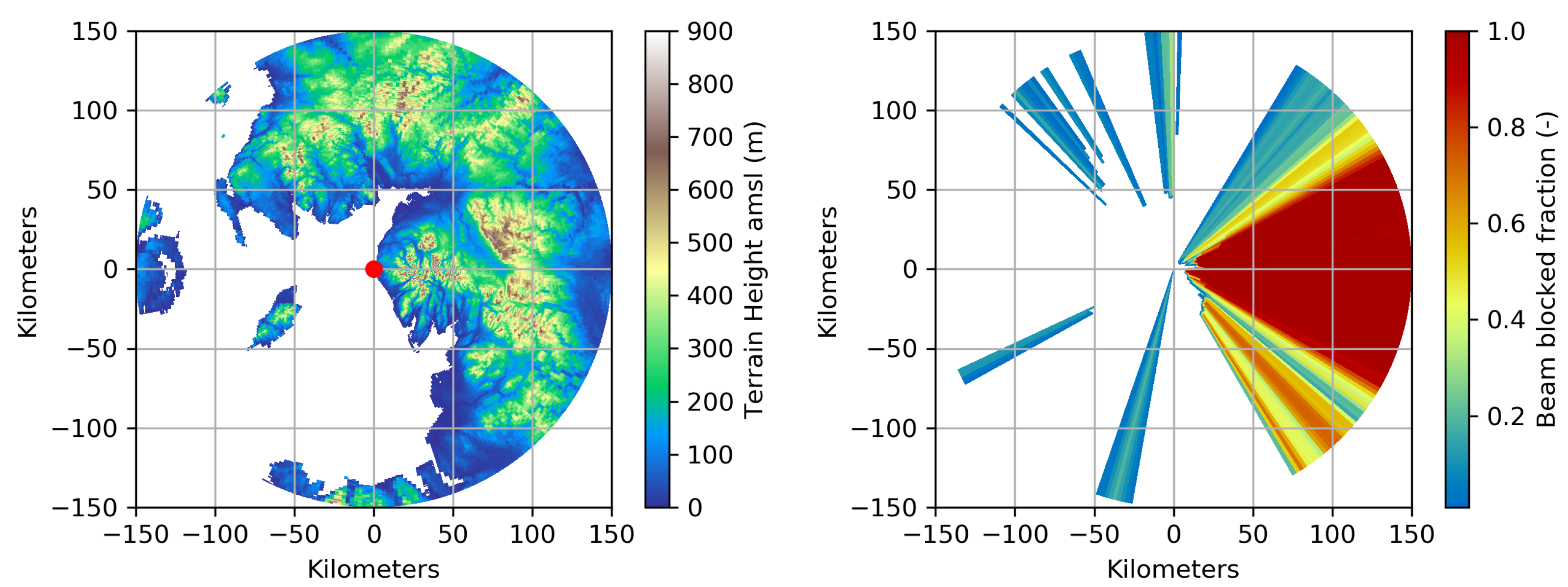
2. Weather Radar Deployment and Data

NXPol-1 is a dual-polarisation mobile X-band research radar that undertakes short (one month) to medium (two year) duration deployments [17]. NXPol-1 is a single-axle trailer-mounted system built by Leonardo Germany GmbH and is capable of operating independently using only the trailer. NXPol-1 is, however, typically deployed on top of two 20-foot (6.06 m) shipping containers, which house radar control computers and additional field campaign supplies while elevating the radar above the surrounding environment (Figure 1). The radar is manually levelled on top of the platform using the trailer’s three adjustable legs: two at the rear and one centred at the front. A dual-axis bubble level provides 0.05° precision per graduation for this process and is mounted on the radar trailer.
The focus of this paper is NXPol-1’s deployment for the Radar Applications in Northern England (RAiN-E) campaign [18]. The radar was deployed from October 2018 to December 2020 at the United Utilities reservoir near Sandwith in Cumbria (54.517°N, 3.615°W). Given the radar’s location, site visits were limited by travel time and typically occurred bi-monthly during the first year of the project. However, following the onset of the COVID-19 pandemic, visits were restricted to emergency situations only for the majority of 2020 (all visits are shown in Table 1). These site visits were primarily to check on site safety or to address minor non-radar issues. During this deployment, the two shipping containers were placed on a scaffold subframe supported on multiple legs with wooden bases constructed over a grassed (soft surface) area (Figure 1). As a result, the radar was routinely re-levelled on its container platform to account for potential settling of the scaffold frame on site. During the entire deployment, NXPol-1 scanned a volume coverage pattern of 10 elevations from 0.5° to 20° (at 0.5, 1, 1.5, 2, 3, 4.5, 6, 7.5, 10 and 20 degrees) followed by a 90° elevation rotation and a semi-hemispheric (180°) range-height indicator (RHI) scan along a fixed azimuth (90° to 270°), with the whole sequence repeating roughly every 6 min. The radar collected dual-polarimetric moments including reflectivity in both horizontal and vertical channels, differential reflectivity, cross-polar correlation coefficient and differential phase shift, along with the signal-to-noise ratios in both channels. A complete set of the radar moments stored can be found in the open-access radar data archive [18].
While NXPol-1’s control software (RAVIS®, Leonardo Germany GmbH, Neuss, Germany) allows offline solar raster scans, they cannot be scheduled to occur at regular intervals; instead, they require manual intervention. These were, therefore, only used during the radar’s initial deployment (to align the azimuth angles to north and check the elevation) and following intervention with the radar system. For a period of four days in September 2020, multiple raster scans were undertaken to provide an additional assessment of the preliminary results that led to this study. The results from these scans cannot be automatically saved for further analysis. In this case, the elevation, azimuth and receiver (Rx) offsets were manually recorded along with the time of the scan. These results can be found in Table A1 in Appendix A.
To further support the analysis presented here, observations made by NXPol-1 at the Chilbolton Observatory (51.145°N, 1.439°W) have also been utilised [19]. The data in question are from a seven-week (2 February 2017 to 21 March 2017) test period during which the radar’s signal-to-noise ratio (SNR) required for data storage was reduced. While the reduction led to the retention of a significant amount of background noise, it also captured a greatly increased number of opportune solar hits at a reduced intensity, which have been useful for analysing the NXPol-1 system.
In addition to data from NXPol-1, raingauge data from the Environment Agency (EA) and Scottish Environment Protection Agency (SEPA) are used to provide external verification of the tilt corrections. Fifteen-minute accumulation time series are used during the study, with data quality-control and processing discussed in Section 5.2.2.

3. Solar Interference Assessment Methodology

Leveraging opportune solar hits collected during standard-volume scanning provides the most accessible option for ongoing monitoring of the pointing of the NXPol-1 radar system and is the only option for assessing historic campaigns. To assess this historic campaign, we implement the multi-step methodology described in the following sections.

3.1. Solar Hit Identification

To determine instances of solar interference within the RAiN-E observations, a combination of open-source radar tools (including the scansun module of BALTRAD’s RAVE toolbox and PyART) were used to parse the CfRadial files and identify interference spikes occurring close to the sun’s position [20,21,22]. The BALTRAD RAVE toolbox implements KNMI’s scansun functionality, first described by Huuskonen and Holleman [12]. For this work, we use unfiltered horizontal reflectivity as input to the RAVE scansun tool. Within the RAVE toolbox, the following process occurs to identify solar hits for further analysis. Firstly, using the ray timestamps within the radar files, a search radius of five degrees around the sun’s known position is calculated and used to find radials that contain a near-continuous (>70%) linear echo (at least 20 km long) at a consistent power level (within 2 dB of a first-estimated mean power value) at high elevations (i.e., higher in altitude than typical weather signals: 8 km for first identification in this case, and 4 km for the second filtered estimation). The RAVE toolbox then converts this power to solar equivalent units (dBsfu) using the radar’s calibration constant and fixed parameters (wavelength, antenna gain, etc.), which allows potential monitoring and calibration of the radar receiver in addition to providing a basic indication of the radar’s pointing accuracy. We then use the pvlib Python package [23] to update the position information from these interference spikes to account for local pressure and temperature information (observed by an automatic weather station deployed with NXPol-1), adjusting the solar position to its apparent position as a result of refraction. These solar identifications (i.e., ’hits’) can then be analysed using the methods described in the following sections to better characterise radar positioning offsets.

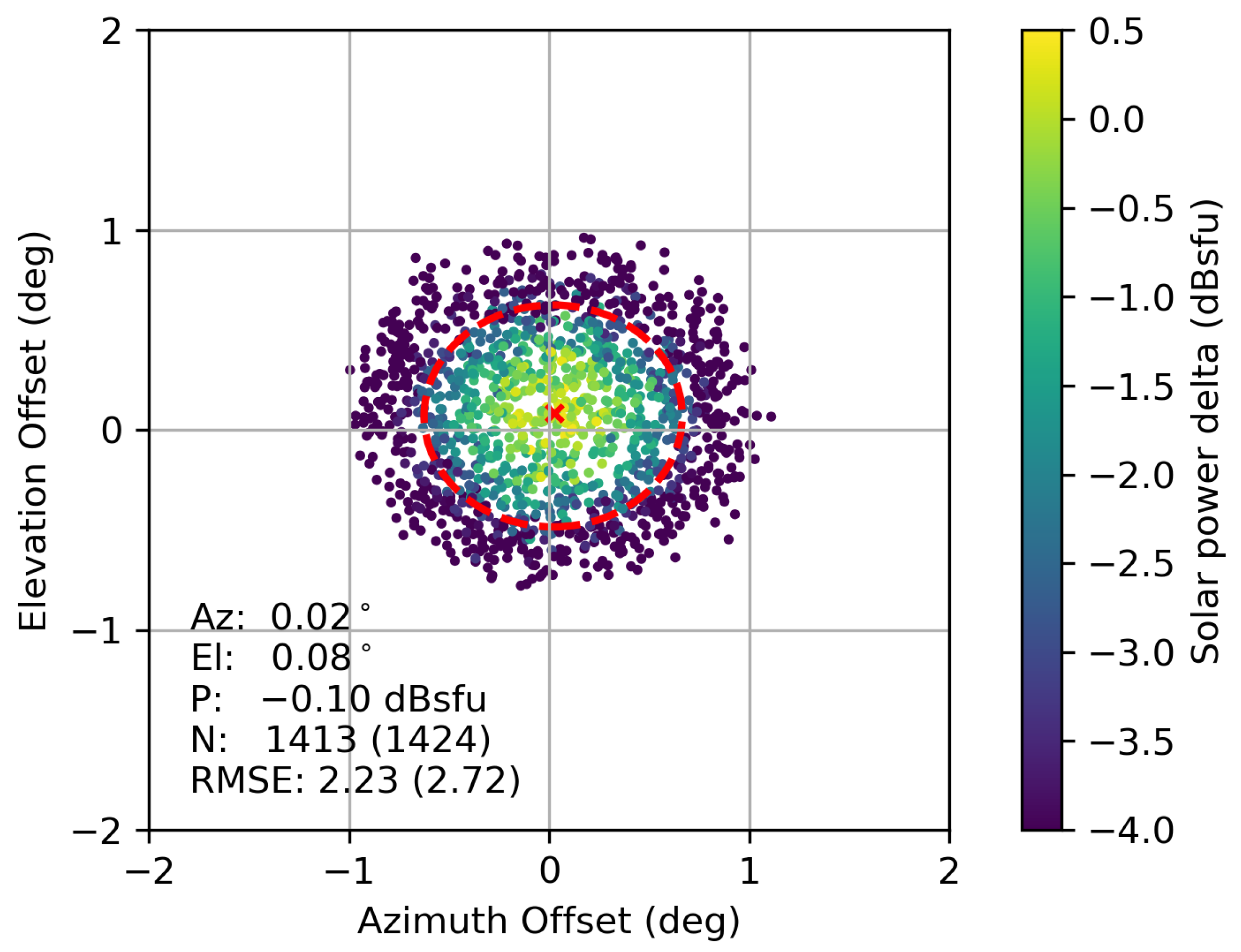
3.2. Application of a Multi-Parameter 2D Gaussian (Bullseye) Fit

To analyse the raw solar hits, a five-parameter model is fitted to their position offsets and recorded solar power. This models the two-dimensional Gaussian form of the combined sun, antenna beam shape and azimuthal beam averaging as first proposed by Huuskonen and Holleman [12]. This approach is commonly referred to as the “bullseye” method, as the solar power decreases from the centre of the disk, producing a bullseye target. The Huuskonen and Holleman [12] method is set out here for completeness. The form of this model is:
p ( x , y ) = a 1 x 2 + a 2 y 2 + b 1 x + b 2 y + c
where p ( x , y ) is the received solar power, x is the difference between the radar azimuth and the solar azimuth (read-sun), and y is the difference between the radar elevation and the solar elevation (read-sun). The equation is described by the linear parameters a 1 , 2 , b 1 , 2 and c, allowing the solar hit data to be fit to it using least squares regression.
From these linear parameters, five physical parameters: azimuth width ( Δ ϕ ), elevation width ( Δ θ ), azimuth offset ( x 0 ), elevation offset ( y 0 ) and peak solar power ( p 0 ) can be calculated through the following equations:
Δ ϕ = 40 log 10 2 a 1 ,
Δ θ = 40 log 10 2 a 2 ,
x 0 = b 1 2 a 1 ,
y 0 = b 2 2 a 2 ,
and
p 0 = c b 1 2 4 a 1 b 2 2 4 a 2 .
Here it is important to note that the azimuth and elevation widths are a function of the convolution of the antenna beam widths and the apparent width of the solar radiation rather than the absolute beam widths of the weather radar, which are already known. To further improve the quality of the fit, outliers are removed based on a comparison to the initial modelled parameters. In this case, any solar hits that deviate by more than 1 dBsfu from the modelled Gaussian form are removed before refitting the model. In the case of both the initial and second (final) fits, the root mean square error (RMSE) is calculated to assess the bullseye model. The RMSE is calculated as follows:
RMSE = Σ n = 1 N ( p n p ^ n ) 2 N
where p n is the observed relative solar flux, p ^ n is the relative solar flux predicted by Equation (1), and N is the total number of solar observations in the analysis window. Calculating the RMSE also allows comparison of different time windows.
During their work, Huuskonen and Holleman [12] used a daily time interval for fitting their data, whereby they were able to obtain 20 to 30 solar hits per day across a range of elevations. In contrast, the NXPol-1’s RAiN-E dataset typically contains fewer than ten hits per day. To mitigate this reduced number of hits and increase the stability of the resulting fit, two modifications are made to their original methodology. Firstly the azimuth and elevation widths ( Δ a z and Δ e l ) are fixed to 1.29° and 1.11° respectively, for the RAiN-E campaign, and secondly, the time windows analysed are lengthened.
The model azimuth and elevation widths used here (1.29° and 1.11°) were derived using the five-parameter fitted model using data from a previous NXPol-1 deployment at Chilbolton Observatory where, during a 7-week period, decreased SNR requirements led to a greater number of low-intensity (estimated solar power below −110 dBm) observations being recorded across a wider elevation and azimuth range (off-axis hits). The additional observations enable a more precise derivation of the 2D power Gaussian as expected considering NXPol-1’s beam width of 0.98°, the antenna rotation speed and the apparent width of the solar radiation source (Figure 2). This step is essential to provide a robust fit with respect to the peak solar power, as otherwise, the narrow sampling of the solar disk when the SNR threshold is increased allows too much freedom for a five-parameter model to broaden the Gaussian through inflation of the azimuth and elevation widths. If an empirical fit is not possible due to sensitivity limitations, theoretically derived values for the model widths can be used instead; Altube [24] covers how to derive these in great detail.
The second modification is to extend the time window used for model fitting to increase the number of observations available. The extension of the time interval has previously been shown to be valid provided that the Sun’s solar emissions do not vary significantly during the period being investigated [12]. While this is generally the case for the duration of the project (brown line, Figure 3), the observations here are converted to relative solar flux using the closest available observations from the Dominion Radio Astrophysical Observatory (DRAO) to reduce the impact of variable solar activity on the resulting fit. Gabella and Leuenberger [25] previously applied such an approach while using solar interference as an absolute calibration source for the radar receiver chain. They employ Tapping’s [26] approximation for 3 cm wavelength to convert DRAO observations from S-band to X-band, and here we take the same approach, which is as follows:
P X = 10 log 10 ( 255 + 0.69 ( F S 64 ) )
where F S is the observed S-band solar flux in solar flux units (sfu), and P X is the equivalent solar flux at X-band in logarithmic solar flux units (dBsfu).
Conversion from absolute observations of solar emission to relative values (termed solar power delta in this work) allows the time windows to be extended without introducing uncertainty due to variability in the Sun’s emissions, increasing the number of observations available and allowing cross-comparison of these multi-parameter power fit estimates with the long-duration tilt estimates described in the following section.

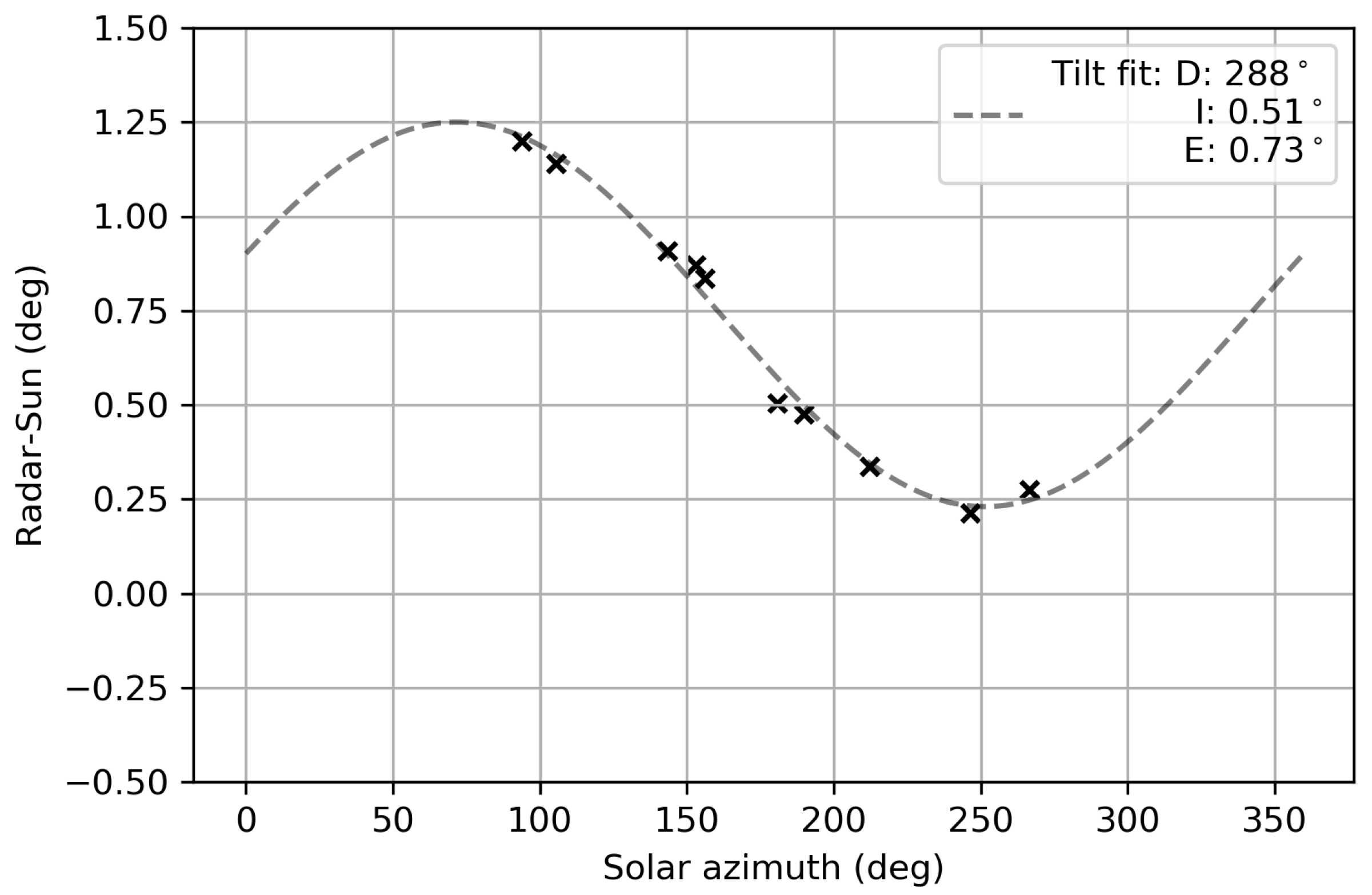
3.3. Using Online Solar Hits to Assess Radar Axis Tilt

The potential for radar axis tilt is assessed here following the ideas presented in Muth et al. [11] and Curtis et al. [16], whereby online solar hits are analysed as a function of solar azimuth. For a visual depiction of these bias sources, see Muth et al. [11], which presents them well. In this case, the tilt is modelled using a simple sine approximation, where only the impact of the tilt on elevation offsets is considered, as the impact on azimuth is significantly smaller for low-elevation angle scanning data at small degrees of tilt. This allows a three-parameter model of the offset
E ϕ = I . cos ( D + ϕ ) + y 0
to be fit to the observed azimuthal distribution of elevation offsets (difference between radar elevation and solar elevation; a function of the pointing biases and position of the radar beam within the solar disk) using least squares regression, for which the three parameters that define the tilt are the orientation of the tilt, declination (D); the magnitude of the tilt, inclination (I); and a fixed elevation offset parameter ( y 0 ) such that the tilt varies between y 0 + I and y 0 I depending on the solar azimuth ( ϕ ). As per Curtis et al. [16], the power of the observed interference is omitted from the analysis, which thus relies on only the positional information.
This approach provides an alternative estimate of the fixed elevation offset ( y 0 ) to the bullseye approach outlined in the previous section. Where there is no observable tilt, these two estimates will be near equivalent due to the expected symmetry of the solar observation. Where they are not equivalent, it provides a strong indication that tilt is impacting the radar system and the bullseye results are being biased by asymmetric observations.

3.4. Combined Methodology

Both the bullseye (2D Gaussian) analysis and the tilt analysis provide complementary information that can inform the most probable correction required for already collected data or the likelihood that corrective maintenance is required when used in real-time. To analyse historical data, the dates of site visits are treated as boundary conditions, where each intervening period is considered individually unless the analysis for consecutive intervals suggests they can be combined. Key factors to consider when determining the correction required are the RMSE of the bullseye fits along with the number of points removed as outliers, the magnitude and direction of the modelled tilt, and the consistency between the fixed offset between the two methods. Another necessary factor to consider is the quality of the radar data as a whole, particularly whether the wider radar observations are consistent with the modelled results. For example, where the results indicate a significant tilt, the melting layer signal observed in a PPI would be more oblate in shape, while patterns would also be visible in ground clutter returns and beam blockage at low elevations. Considering each of these factors in turn, high original RMSE’s along with large reductions in RMSE between the two fits and removal of numerous points by the 1 dB filter are indicative of potential tilt, where the bullseye model fails to fit the observations well due to the points having a bi-modal distribution. This leads to the 2D Gaussian being fit to pass through the two modes with a peak between them, thus also overestimating the solar power delta and leading to filtering of points that lie between the two modes. The declination of the tilt also needs careful consideration, as declination results aligned near north could be due to the semi-sinusoidal path of the sun through the sky, which becomes particularly evident at higher latitudes. In this case, the slow procession of the sun through the sky at relatively low elevation angles creates a sinusoidal track in the offset results, which can lead to the misdiagnosis of tilt aligned to north, particularly as the solar power delta of these hits is not considered when assessing radar axis tilt. The magnitude of the inclination is easier to consider, with high magnitudes less likely to occur and easier to visually confirm with inspection of PPIs at low elevation. For example, visual inspection of PPIs during widespread stratiform precipitation can indicate whether beam blockage has increased preferentially in a certain direction, which could be an indicator of tilt. This may also be visible as an elliptical or oblate melting-layer signal within the PPIs, particularly when viewing a field such as the co-polar correlation coefficient as the sweep no longer cuts through the melting layer at a constant range for each azimuth (care must be taken that this is not a function of heterogeneous temperature profiles though). Through consideration of these factors, it is possible to determine a pointing correction for historical data even when time periods are data sparse; this leads to improvements in radar data quality, as will be discussed in the following two sections.

4. Results of the Tilt Estimation Method

Figure 3 shows the positional offsets (radar recorded position minus solar known position) of the identified solar interference observations from the RAiN-E project through time, with the azimuth record shaded by solar elevation in Figure 3 (Panel A) and the elevation record conversely shaded by solar azimuth in Figure 3 (Panel B) to highlight any potential dependencies through time. For an accurately pointing radar with zero tilt, the identified solar interference would vary around zero offset in both azimuth and elevation as the radar traverses the solar disk. However, these results show significant variation in both directions. The elevation time series consistently shows a positive offset, which increases in magnitude from July 2019 and then splits in summer 2020 with observations of low/high azimuths displaying increasing/decreasing trends, respectively. These initial findings indicate significant errors (>0.2°) in the radar pointing accuracy, which can potentially be attributed to changes in NXPol-1’s tilt. It is also noticeable that solar hits are observed more frequently after July 2019, when the radar receiver board was replaced due to a fault, which also coincides with a change in the relative offset between the radar-observed solar flux and the equivalent observations from DRAO, as shown in Figure 3 (Panel C).
Also shown in Figure 3 are the site visits detailed in Table 1. These interventions subdivide the time period into the nine periods shown in Table 2, which vary in length from 7 to 344 days, with only the longest sector (Period 8) exceeding Curtis et al. [16]’s recommended length of 16 weeks for a stable diagnosis of antenna tilt. Table 2 also indicates that NXPol-1 observed significantly fewer (fewer than half as many per day) solar interference spikes than other systems outlined in the literature, particularly during the first eight months of the deployment, as a result of the reduced sensitivity of NXPol-1 and the scanning geometry.
To analyse each of these periods, the combined methodology outlined above is applied to each separately. Figure 4 is an example of this approach for Period 8, while Table 3 summarises the results for all of the time periods. To determine the correction for each time period, an informed assessment of the consistency of these results is undertaken. To demonstrate this, we here take Period 8 (Figure 4) as a detailed example, from which it can be observed that:
  • A significant number (>40%) of points are excluded between the first and second fit of the bullseye model, which is accompanied by a large reduction in the RMSE from 1.34 to 0.50 (seen on the lower-right panel of Figure 4). This suggests that a Gaussian model with fixed offsets does not model the observations well.
  • The estimated solar power offset of 1.64 dBsfu exceeds expectations based on Figure 3, again indicating the fitted model is not characterising the observations.
  • The estimated elevation offsets of the two approaches agree very closely (within 0.05 ) despite the limitations of the bullseye fit due to averaging through time, which increases confidence in the results.
  • The magnitude of the inclination is significant enough (>0.1°) to impact radar observations through time without being such a severe deviation from the previous period (>0.5°) as to prompt immediate intervention.
  • The bullseye figure has a v-shaped distribution of points, with more-extreme elevation offsets also having more positive azimuth offsets. This is a particularly unusual distribution of points, even for a system with tilt, and is an indication that the offsets (either tilt/fixed or both) have changed through time, particularly as the solar flux delta is high within these distributions.
  • Further evidence of time-variant offsets are the broad distribution of points across an extended elevation offset range (>1.0°, the typical maximum bullseye size given the radar sensitivity during the project) between 60 and 120 azimuth and the time-series plot (Figure 3), where the distribution of points is clearly asymmetric around the summer solstice. In the case of a system with a constant tilt through time, you would expect a more-symmetrical distribution as the azimuths sampled within the radar volume during spring are the same as those sampled during autumn.
Period 8 is unique in the dataset as it is the only period to be longer than the 16 week interval recommended by Curtis et al. [16] and is also the only time period during which offline raster scans were taken, which act as a complementary assessment. A total of ten raster scans (Table A1) were undertaken across a 3-day period from 14 to 17 September 2020, covering elevation angles from 5 to 40 degrees and an azimuth range of 173 degrees (94° to 267°). These results also show the elevation offset to be azimuthally dependent, where the fitted tilt model has a declination of 288.4°, an inclination of 0.51° and a fixed elevation offset of 0.74°(Figure A1). While these are roughly comparable to the results of the analysis of solar hits collected during normal operation of the radar, there is a factor of two increase in the inclination compared to the period as a whole. This is accompanied by a subtle shift in the declination, perhaps indicating the radar platform as a whole or some component of it (trailer/scaffold etc.) sank during this time period (see later discussion).
Given the significant change in magnitude and the length of the data record for Period 8, it has been split into two periods (5 November 2019 to 15 June 2020 and 15 June 2020 to 14 October 2020) to derive the final correction. The final 16 weeks of the period (from 15 June 2020) were analysed separately, and a tilt model of 261° declination, 0.48° inclination and 0.58° offset was derived, which is similar to the raster scan observations if refraction correction is applied to those results. The results are not a closer match, as the split into two time periods does not fully characterise the changes in pointing offsets occurring during this period. Alternative approaches to characterising the variable tilt during Period 8 were explored, including a short-duration (7-day) moving window approach and splitting the period into shorter arbitrary time windows, but given the potential non-linearity of the tilting system (it is not clear whether the changes are step-changes at fixed points in time or rather more gradual changes that may or may not have a constant rate of change) and the greater uncertainty of small time windows for tilt estimation, the simple approach of an arbitrary split was used for the final correction. The final fitted tilt model for the first part of Period 8 is shown in Table 4, which shows the final corrections used for all of the time periods.
Each of the other time periods was assessed using the metrics in Table 3 along with additional observations and expert intuition, leading to the final corrections shown in Table 4. Given the small yet non-negligible impact of tilt on the azimuth offset, the final azimuth corrections were recalculated using a bullseye model after undergoing tilt and elevation offset correction. These tilt corrections were then applied to the data within each time period such that 10 different corrections were applied during the whole duration of the project. In almost all cases, the tilt model approach was employed: however, notable exceptions are as follows. Firstly, Periods 2 and 3 were combined, using a single correction for both due to the closeness of their original results in Table 3. During this combined period, the fitted tilt model was also discounted as more general radar observations (individual reflectivity PPIs and monthly echo occurrence plots, for example) showed no evidence of a pointing offset in excess of 1.0°, with this result highlighting the difficulty of applying a tilt correction at high latitudes in winter (see discussion). The other period for which the tilt model was discounted was Period 5, which was the second-shortest period, with a low number of solar hits per day. In this case, the bullseye fit was taken as a final correction based on analysis of polar volume radar data and processed data products (see verification). Given all but one of the corrections is based on a time interval significantly shorter than the 16 weeks recommended by Curtis et al. [16], additional verification of the correction has been considered prior to acceptance of the corrections for application to future work. The following section describes that approach and its results.

5. Pointing Correction Verification

While the methods utilised here have a strong theoretical underpinning and have previously been implemented successfully for identifying radar defects, there still remains a degree of underlying uncertainty for the results shown in Table 4 that is difficult to quantify due to the data sparsity in many time periods and the location of the radar at a high latitude that limits the observed solar hits to a narrow azimuth range in winter. As a result, post-correction verification is an essential step for understanding the results and the limitations of the underlying methods for high-latitude locations. Here we present two approaches: the first based on reanalysis of the solar hits themselves and the second being an analysis of radar quantitative precipitation estimates (QPEs) before and after correction. The first approach can be considered a simple sense check of the results, while the second approach provides a much wider verification but is prone to its own uncertainties. Alternative approaches were also considered, such as an analysis of retrieved melting layers (again prone to a wide degree of uncertainty due to atmospheric variations), but the two presented here are more robust and provide additional verification to support the derived corrections.

5.1. Solar Hit Reanalysis

The simplest method for verifying the correction is to consider its impact on the solar hits themselves. Re-analysis of the solar hits using the 2D Gaussian fit model indicates an increase in consistency across the field campaign (even though the power differential has not been addressed). Figure 5 shows these fits for the entire campaign both before and after correction. In addition to the derived offsets now being near zero, there is an improvement to both the first and second fit RMSEs along with the second fit now retaining all but seven of the data points. While these results are a strong indication that the correction has improved the pointing accuracy of the data, they do not provide independent verification; this is considered in the following section on radar QPE.

5.2. Radar QPE and Verification with External Data

Assessing the impact of tilt and its correction on the accuracy of QPEs allows external verification of the tilt correction using ground data while also being indicative of the benefit of the correction for future end users. The assessment conducted here compares radar QPEs to precipitation surfaces produced by the interpolation of raingauge networks and assesses performance by comparing areal averages calculated over hydrological catchments. This approach was used in preference to a direct assessment against raingauge measurements at point locations because catchment averages are more indicative of whether improvements due to the tilt correction will be carried forward to a final use such as hydrological modelling, and they are also less sensitive to any potential localised radar artefacts. The verification was undertaken considering the project as a whole but also for each individual time period. This allows each individual correction to be assessed independently while also considering whether the overall performance of the data improves for the project.
The verification is not a perfect assessment of the tilt correction given the underlying complexities of radar QPE [6,27], but here we demonstrate the value of this approach when dealing with a polarimetric processing chain, which is described in the following section. This verification is also only possible due to the orographic environment the radar was deployed in, where partial beam blockage (PBB) from high topography at multiple ranges from the radar has a significant impact on radar visibility and power returns. We demonstrate this in Section 5.2.3, where the widespread availability of rainfall observations from regions of varying blockage severity is illustrated, followed by a discussion of the results of the comparison and their value for assessing the tilt correction.

5.2.1. Radar QPE Methodology

Quantitative precipitation estimates are generated for this study using the processing methodology developed for NXPol-1 and previously used to assess QPE in northern Scotland [28,29,30]. The methodology first corrects for PBB with a high-resolution DEM (SRTM 1-arc second global data [31]) using the open-source Wradlib processing library [32]. Figure 6 shows the terrain altitude within 150km of the radar location along with the resulting blocked beam fraction assuming a constant elevation angle of 0.5° for the entire sweep. In this work, the PBB correction has been modified to allow variation within a sweep of the elevation angle, where the correction is applied with a precision of 0.1° in elevation. After correction for PBB, the reflectivity data are cleaned using a fuzzy-logic classifier to remove non-meteorological echoes and are then corrected for attenuation and converted to precipitation intensity using the Marshall–Palmer relationship [33]. The QPEs are solely derived using a reflectivity-only estimate of precipitation intensity rather than incorporating dual-polarisation estimators in order to reduce the complexity of the subsequent results given other radar moments are immune to partial beam blockage. Two estimates are compared here: one where PBB is corrected using the radar’s recorded azimuth and elevation data as truth and one where tilt correction is applied before PBB correction. All other processing steps are identical for both estimates. As per Wallbank et al. [28], after precipitation intensity is estimated for all radar sweeps, the volume is flattened using a fixed lowest usable elevation look-up table and then remapped from polar coordinates onto a 1 km Cartesian rectilinear grid using the area-weighted average of all 2D polar radar pixels intersecting with each Cartesian grid cell. The gridded precipitation intensities (produced approximately every 6 min) were then accumulated using a simple trapezoidal rule to produce hourly gridded accumulations that were used for comparison to raingauge observations (as detailed below). Any period of greater than 10 min without a radar scan was treated as missing.

5.2.2. Verification Using External Data

Raingauge network data over England and Scotland were obtained from the Environment Agency and Scottish Environment Protection Agency, respectively, and processed separately using the methods described in Wallbank et al. [28]. Briefly, this entailed an initial quality control step followed by spatial interpolation of the raingauge values using the multiquadric method to produce 1 km-resolution precipitation grids that were accumulated to an hourly timestep. These 1 km grids match those produced for the radar data in the previous section. In total, there were 233 raingauges within 150 km of the radar site.
Verification was performed by comparing catchment averages of the hourly gridded radar QPE and raingauge surfaces over the 215 catchments outlined in Figure 7. Of these, 85 catchments (shown with bold outlines on Figure 7) have a mean lowest usable elevation for the radar beam of less than 2 km, indicating that the beam elevation should not be considered excessive for these catchments. Several statistical quantities were then computed over each catchment in order to assess different aspects of the performance of the radar QPE.
The first statistic,
percentage bias = 100 % p i P i P i ,
assesses the relative difference in the total depths of water between radar and raingauge QPE, where p i and P i are the hourly catchment averages of the radar QPE and raingauge interpolation “truth”, respectively, and angular brackets, , denote temporal averaging over all non-missing timesteps. A second statistic,
MAPE = 100 % | p i P i | P i ,
was used to assess relative error in the radar QPE. It was chosen in preference to alternatives such as the R 2 efficiency (Nash–Sutcliffe Efficiency) as it is insensitive to the zero-inflated nature of precipitation data (which has a value of zero for a considerable portion of timesteps). A final statistic, the correlation coefficient, r, was used to assess the size of errors in the data independent of any overall bias. Note that the last two statistics are sensitive to the choice of the hourly timesteps used in the calculation. This was deemed to be a relevant timescale over which accurate precipitation data would be needed for modelling flood hydrology in this region.

5.2.3. QPE Correction Results

Figure 7 displays the change in radar QPE performance after tilt correction, assessed over the whole campaign period. Precipitation in this region, as calculated using the raingauge network, varies considerably. The wettest catchments are in the west, with the wettest catchment totalling an average of 6562.3 mm of precipitation during the campaign period (equivalent to 3078.6 mm/yr), compared to the driest catchments, in the east, with precipitation totals as low as 1281.8 mm (equivalent to 601.3 mm/yr). This trend is further exaggerated in the radar QPE due to the high radar beam elevation necessary in the east due to the interposing Lake District fells (Figure 6). This results in the radar beam overshooting large portions of the precipitation in this region and consequently produces strongly negative biases and poor MAPE and correlation in the radar QPE regardless of any tilt correction. Because of this, it is often instructive to limit the analysis to those 85 catchments, outlined in bold in Figure 7, with a Lowest Useable Elevation (LUE) of less than 2 km. Here, vertical processes (including melting, orographic enhancement and advection) are less likely to influence the QPE comparisons [28], and they additionally tend to be closer to the radar (due to the radar beam propagating at a positive elevation angle), thus limiting the influences of beam broadening, reduced radar sensitivity and partial beam filling on the QPE comparisons.
The percentage biases shown in Figure 7 are negative to a greater or lesser extent for all catchments, including those with LUEs less than 2 km. However, the application of the tilt correction does result in a systematic improvement in bias over the entire radar domain, including a median increase in bias of 11% for catchments with LUEs less than 2 km. This is expected given the majority of the tilt correction periods lead to an increase in the magnitude of the partial beam blockage correction across the entire domain. This is due to all the computed elevation offsets (static + tilt) having a positive sign, which indicates the radar is always pointing at a lower elevation than requested. As the elevation angle is lower than requested, the partial beam blockage correction applied in the first instance is insufficient and must increase in magnitude to correct for the elevation offsets. The absence of positive percentage biases across all catchments in the corrected QPE is a strong indicator that the increase in tilt correction is not an overestimation, which would introduce too much beam blockage correction and hence positive rainfall biases.
The benefit of using the tilt correction is also clear in the general trend to lower MAPE. This statistic displays a median reduction of 5% for catchments with LUEs less than 2 km. There are, however, two catchments in Scotland that suffer a slight (less than 3%) increase in MAPE, which highlights the spatially distributed impact of applying a tilt correction that is strongly dependent on local topography.
The application of the tilt correction produces a more mixed effect on the correlation coefficient, with some of the catchment with LUEs less than 2 km displaying a modest increase (five display increases > 0.05 ), some displaying slight decreases (three display decreases < 0.02 ) and the majority displaying little change, particularly among those with acceptable correlation coefficients to begin with. Given the tilt correction changes temporally, this suggests that the variability it creates from period to period is not the dominant control for the correlation of the QPE with surface observations, and that the correction is not causing additional decorrelation across the dataset.
Figure 8 summarises the performance of radar QPEs both before and after tilt correction for each of the correction periods in turn. In this case, only the 85 catchments with LUEs below 2km are included. The limited influence of tilt correction on the correlation coefficient found for the full campaign is repeated during each of the periods. It is also noticeable that the correlation during each period is higher than that for the dataset as a whole, indicating the temporal variability of radar QPE performance, particularly when using a fixed Z-R relationship. Considerably larger changes are observed in the percentage bias and the MAPE, both of which display improvement for all periods except Period 1. Period 1’s worsening performance is driven by an increasingly negative percentage bias, perhaps suggesting that the positive changes to radar elevation pointing lead to an under-correction of partial beam blockage. Period 1 is, however, only seven days long, and the correction is based on only 40 solar hits, suggesting a limitation of the methodology, particularly when it indicates significant changes to pointing are required. Additionally, seven days is a very limited period over which to assess the data. Results for Period 5, only 13 days long, should also be treated with caution.
The performance clearly varies across the time periods, with a possible decline in performance seen later in the project (periods 6 to 8b, in particular), with an increasingly negative percentage bias, an increase in MAPE and a reduction in correlation. While the tilt correction has a positive effect on these results, it does not fully restore performance. This is likely due to the increasing occurrence of total beam blockage that cannot be corrected. Figure 6 clearly shows total beam blockage occurring at 0.5° elevation to the east of the radar where there is high topography close to the radar location. This total beam blockage occurs more frequently as the elevation offset (both fixed and due to tilt) increases because the radar’s actual elevation angle is lower than the one requested (a nominal elevation angle of 1.0° is actually scanning at 0.5° or lower in some cases). To mitigate this error, one option would be to introduce dynamic elevation selection into the processing, which may recover more information from the dataset; however, this would come from higher elevations, which then have a greater uncertainty due to the impacts of horizontal advection, phase changes and vertical profiles of reflectivity. This highlights the requirement to monitor tilt in real-time, as it can have a fundamental, uncorrectable impact on radar QPE quality depending on its magnitude and the local topography.

6. Discussion and Conclusions

Through the combination of two analysis techniques, this work derives a pointing offset correction for an historical dataset collected by NXPol-1. The study can be generalised to provide recommendations for both the correction of historical data and for future monitoring of radar systems, with a particular focus on deployments/radars at high latitudes.

6.1. Review of the Analysis Methods and Results

The two analysis techniques applied here (a 2D Gaussian model and a sinusoidal tilt model) complement one another through the introduction of quality-of-fit metrics allowing them to be applied to shorter time periods. The methods are of particular relevance to mobile research radars, which are often deployed for short-duration research projects and are more likely to be deployed on less-stable structures than long-term, static operational weather radar. The combination of techniques is especially important given the relatively high latitude of the radar (greater than 50°), which introduces additional uncertainty into the tilt methodology of Curtis et al. [16] due to the concentration of solar hits within a narrow azimuth range (southerly in this case) and the sinusoidal procession of the sun through the sky at lower elevations during this period. Figure 4 clearly shows these artefacts between azimuths of 165° and 195° where the sun is at a low enough elevation to generate a collection of solar hits at the same radar-recorded elevation angle. It is particularly in this context that alternative sources of information are useful: in this case, the additional QPE verification described in Section 5 can be used to assess the plausibility of the derived corrections relative to raingauge observations. In the case of NXPol-1 and the RAiN-E datasets, the improvement in percentage bias and MAPE of the radar QPE for the majority of catchments across the region provides external confidence that the corrections are accurate. In the context of tilt corrections, where QPE variation largely results from changes in partial beam blockage correction, the use of catchment average precipitation rather than gauge point estimates is preferable as it provides a degree of averaging that compensates for the highly spatially variation and non-linear nature of beam blockage change, the varying locations of gauges, and the known variability in radar for point observation comparisons.
While the corrections can be deemed plausible following verification, determining the exact cause of the tilt variation, particularly during Period 8 where no manual intervention occurred, is not possible. The most likely explanation is a settling of the scaffold construction through time, possibly compounded by changes in soil conditions. Other possibilities are movement of the radar’s own legs during such an extended deployment without intervention or, less-likely, differential heating of the radar and containers, leading to movement of the system. While deployment on a concrete foundation would be preferable for future field campaigns, the techniques presented here, along with the following recommendations, would make it easier to manage such an uncertain, soft-ground deployment in the future. In all cases, regular monitoring and site visits would be recommended.

6.2. Recommendations

Based on the analysis presented here, we have the following recommendations, which are applicable to both NXPol-1 and weather radars in general, with a particular focus on higher latitudes.
All weather radars should be monitored for potential errors in pointing accuracy—both mobile research systems and fixed-location operational systems—as demonstrated by this work along with previous studies. During installation/commissioning of radar systems, we recommend more traditional approaches to radar levelling are taken, including the use of manual level assessment using gunners quadrants or high-precision levels. Chandrasekar et al. [34] provide detailed instructions that could be followed to manually assess the tilt of a radar system during deployment. To complement these techniques, we recommend offline raster scans be undertaken on multiple days covering a broad azimuth range to give the highest confidence that the system is level from the beginning. We would also recommend that the results from these raster scans be saved/recorded for further analysis, as demonstrated by Frech et al. [10]. We would also encourage all radar manufacturers to add this functionality to their raster scan procedures in cases where it does not already exist. The online approaches detailed here do not provide results quickly enough to be sufficient for accurate installation.
After installation, record as much data as possible by using a low minimum SNR (or collecting received power/equivalent reflectivity at every range gate if possible) to increase the number of solar hits obtained. This is particularly important for radar systems with a lower sensitivity due to receiver architecture or antenna gain (like X-band systems, which typically have smaller antennas). If collected, online solar hits provide a reliable method for assessing pointing accuracy. We recommend analysing these on an ongoing basis and under standard conditions. Tilt analysis can augment these results once a sufficiently long data sample has been collected. However, if a radar system is found to deviate beyond acceptable pointing accuracy limits using the ongoing monitoring, raster scans should be introduced to assess the potential for tilt more rapidly, as a drift in fixed offset through time and a change in tilt can both produce a comparable signal when assessing ongoing 2D Gaussian fits. Alternatively, site intervention may be the best option if a system is observed to drift in time.
For radar systems at higher latitudes, solar hits may not be a sufficient option for monitoring—at least without additional information. This is particularly true during winter, where the possibility exists that some radars may observe few to no solar hits. For these systems, potential options are the use of indirect assessments, such as analysis of QPE error structures. The use of radar QPE may only be a viable option for verification in areas of complex topography, where partial beam blockage is a potential component of the QPE variability. In flatter regions, the impact of radar tilts of this magnitude on QPE would be significantly lower, though they may lead to an increase in ground clutter returns. This could potentially be monitored or evaluated using the relative calibration adjustment (RCA) technique of Silberstein et al. [35], provided careful consideration of other sources of reflectivity fluctuation are also considered. Another option would be to use dedicated clutter scans of a fixed target such as a television tower or similar, Gabella [36] has been actively pioneering such an approach for dual-polarisation monitoring. It is also likely that independent monitoring of pedestal tilt would be advantageous through the use of a digital inclinometer, for example. While this would allow monitoring of pedestal tilt, it may not capture encoder errors and, therefore, should be viewed as an additional measure rather than a one-stop solution.

Author Contributions

Conceptualization, D.D. and R.R.N.III; methodology, software, formal analysis and visualisation, D.D.; verification J.R.W. and D.D.; data curation D.D., J.R.W. and L.B.; writing—original draft preparation, D.D.; writing—review and editing, D.D., L.B., J.R.W. and R.R.N.III; supervision and funding acquisition, R.R.N.III; All authors have read and agreed to the published version of the manuscript.

Funding

This work was funded by the National Environment Research Council (NERC) grant HydroJULES (NE/S017380/1) and the Environment-Agency-funded RAiN-E project.

Data Availability Statement

Raingauge data used in this study were provided by the Environment Agency (England) and Scottish Environment Protection Agency (Scotland) through open data requests. The radar data used in this study are openly available from the Centre for Environmental Data Analysis (CEDA) archive [18,19]. The corrected data presented in this study are available on request from the corresponding author, as they are not yet a finalised published dataset.

Acknowledgments

The authors would like to thank Robert Moore and Steven Cole for the many valuable discussions on the subject of this work. The authors would also like to acknowledge the Atmospheric Measurement and Observation Facility (AMOF), which is funded by the Natural Environment Research Council (NERC), for providing the radar data. We would also like to thank all those who assisted with the radar deployment at Sandwith, particularly Paul Hodgson and Mark Fawcett from United Utilities and David Snaith from the Environment Agency. The time, comments and suggestions of Patricia Altube Vázquez and two anonymous reviewers are also greatly appreciated.

Conflicts of Interest

The authors declare no conflict of interest. The funders had no role in the design of the study; in the collection, analyses, or interpretation of data; in the writing of the manuscript, or in the decision to publish the results.

Appendix A. Raster Scan Results

The following results (Table A1) were manually recorded from raster scans manually initiated during a short period of the project following some initial analysis of online solar hits. The raster scan procedure is an automated procedure within the Leonardo Ravis operating software that does not provide for saving of the results automatically and provides no functionality beyond a screenshot for saving the results from scanning the solar disk itself (to analyse beam squint, for example). These results were then also used to assess radar tilt (Figure A1).
Table A1. Recorded results from the Leonardo raster scan procedure.
DateTime (UTC)Azimuth OffsetElevation OffsetRx Offset
14 September 202012:12:180.7780.504−1.089
15 September 202010:42:370.6510.871−1.086
15 September 202010:53:540.6630.835−0.966
16 September 202010:07:390.5650.908−0.756
16 September 202012:40:040.7540.476−0.79
16 September 202013:54:230.6550.337−1.281
16 September 202016:10:300.4150.213−1.008
16 September 202017:45:140.3280.274−0.994
17 September 202006:33:580.2141.199−1.226
17 September 202007:30:060.2581.140−1.296
Figure A1. Manual raster scan results plotted as solar azimuth versus elevation offset (black crosses) along with the fitted tilt result (grey dashed line), with the declination (D), inclination (I) and fixed elevation offset (E) shown on the plot legend.
Remotesensing 15 05637 g0a1

References

  1. Sokol, Z.; Szturc, J.; Orellana-Alvear, J.; Popová, J.; Jurczyk, A.; Célleri, R. The Role of Weather Radar in Rainfall Estimation and Its Application in Meteorological and Hydrological Modelling—A Review. Remote Sens. 2021, 13, 351. [Google Scholar] [CrossRef]
  2. Ryzhkov, A.V.; Snyder, J.; Carlin, J.T.; Khain, A.; Pinsky, M. What Polarimetric Weather Radars Offer to Cloud Modelers: Forward Radar Operators and Microphysical/Thermodynamic Retrievals. Atmosphere 2020, 11, 362. [Google Scholar] [CrossRef]
  3. ISO 19926-1:2019; Meteorology—Weather Radar—Part 1: System Performance and Operation; Technical Report. International Organization for Standardization: Geneva, Switzerland, 2019.
  4. Harrison, D.; Georgiou, S.; Gaussiat, N.; Curtis, A. Long-term diagnostics of precipitation estimates and the development of radar hardware monitoring within a radar product data quality management system. Hydrol. Sci. J. 2014, 59, 1277–1292. [Google Scholar] [CrossRef]
  5. Bech, J.; Gjertsen, U.; Haase, G. Modelling weather radar beam propagation and topographical blockage at northern high latitudes. Q. J. R. Meteorol. Soc. 2007, 133, 1191–1204. [Google Scholar] [CrossRef]
  6. Germann, U.; Boscacci, M.; Clementi, L.; Gabella, M.; Hering, A.; Sartori, M.; Sideris, I.V.; Calpini, B. Weather Radar in Complex Orography. Remote Sens. 2022, 14, 503. [Google Scholar] [CrossRef]
  7. Frech, M.; Mathijssen, T.; Mammen, T.; Gabella, M.; Boscacci, M. Monitoring of Weather Radars: Lessons Learned from WXRCalMon17 & WXRCalMon19, and Recommendations. Work Package OA1, EUMETNET OPERA 5. 2020. Available online: https://www.eumetnet.eu/wp-content/uploads/2021/07/opera_monitoring_recommendations_1_21.pdf (accessed on 3 March 2022).
  8. Holleman, I.; Huuskonen, A. Analytical formulas for refraction of radiowaves from exoatmospheric sources. Radio Sci. 2013, 48, 226–231. [Google Scholar] [CrossRef]
  9. Darlington, T.; Kitchen, M.; Sugier, J.; de Rohan-Truba, J. Automated real-time monitoring of radar sensitivity and antenna pointing accuracy. In Proceedings of the 31st Conference on Radar Meteorology, Seattle, WA, USA, 6 August 2003; pp. 538–541. [Google Scholar]
  10. Frech, M.; Mammen, T.; Lange, B. Pointing Accuracy of an Operational Polarimetric Weather Radar. Remote Sens. 2019, 11, 1115. [Google Scholar] [CrossRef]
  11. Muth, X.; Schneebeli, M.; Berne, A. A sun-tracking method to improve the pointing accuracy of weather radar. Atmos. Meas. Tech. 2012, 5, 547–555. [Google Scholar] [CrossRef]
  12. Huuskonen, A.; Holleman, I. Determining Weather Radar Antenna Pointing Using Signals Detected from the Sun at Low Antenna Elevations. J. Atmos. Ocean. Technol. 2007, 24, 476–483. [Google Scholar] [CrossRef]
  13. Altube, P.; Bech, J.; Argemí, O.; Rigo, T.; Pineda, N. Intercomparison and Potential Synergies of Three Methods for Weather Radar Antenna Pointing Assessment. J. Atmos. Ocean. Technol. 2016, 33, 331–343. [Google Scholar] [CrossRef]
  14. Huuskonen, A.; Saltikoff, E.; Holleman, I. The Operational Weather Radar Network in Europe. Bull. Am. Meteorol. Soc. 2013, 95, 897–907. [Google Scholar] [CrossRef]
  15. Holleman, I.; Huuskonen, A.; Gill, R.; Tabary, P. Operational Monitoring of Radar Differential Reflectivity Using the Sun. J. Atmos. Ocean. Technol. 2010, 27, 881–887. [Google Scholar] [CrossRef]
  16. Curtis, M.; Dance, S.; Louf, V.; Protat, A. Diagnosis of Tilted Weather Radars Using Solar Interference. J. Atmos. Ocean. Technol. 2021, 38, 1613–1620. [Google Scholar] [CrossRef]
  17. Neely, R.R., III; Bennett, L.; Blyth, A.; Collier, C.; Dufton, D.; Groves, J.; Walker, D.; Walden, C.; Bradford, J.; Brooks, B.; et al. The NCAS mobile dual-polarisation Doppler X-band weather radar (NXPol). Atmos. Meas. Tech. 2018, 11, 6481–6494. [Google Scholar] [CrossRef]
  18. Bennett, L. RAIN-E: NCAS Mobile X-Band Radar Scan Data from SANDWITH, Near Whitehaven in Cumbria, UK, Version 1; Centre for Environmental Data Analysis: Chilton, UK, 2021. [Google Scholar] [CrossRef]
  19. Bennett, L. NCAS Mobile X-Band Radar Scan Data from 1st November 2016 to 4th June 2018 Deployed on Long-Term Observations at the Chilbolton Facility for Atmospheric and Radio Research (CFARR), Hampshire, UK; Centre for Environmental Data Analysis: Chilton, UK, 2020. [Google Scholar] [CrossRef]
  20. Michelson, D.; Henja, A.; Ernes, S.; Haase, G.; Koistinen, J.; Ośródka, K.; Peltonen, T.; Szewczykowski, M.; Szturc, J. BALTRAD Advanced Weather Radar Networking. J. Open Res. Softw. 2018, 6, 12. [Google Scholar] [CrossRef]
  21. Helmus, J.; Collis, S. The Python ARM Radar Toolkit (Py-ART), a Library for Working with Weather Radar Data in the Python Programming Language. J. Open Res. Softw. 2016, 4, e25. [Google Scholar] [CrossRef]
  22. Heistermann, M.; Collis, S.; Dixon, M.J.; Giangrande, S.; Helmus, J.J.; Kelley, B.; Koistinen, J.; Michelson, D.B.; Peura, M.; Pfaff, T.; et al. The Emergence of Open-Source Software for the Weather Radar Community. Bull. Am. Meteorol. Soc. 2015, 96, 117–128. [Google Scholar] [CrossRef]
  23. Holmgren, W.F.; Hansen, C.W.; Mikofski, M.A. pvlib python: A python package for modeling solar energy systems. J. Open Source Softw. 2018, 3, 884. [Google Scholar] [CrossRef]
  24. Altube, P. Procedures for Improved Weather Radar Data Quality Control. Ph.D. Thesis, Universitat de Barcelona, Barcelona, Spain, 2016. Available online: http://hdl.handle.net/10803/400398 (accessed on 28 November 2023).
  25. Gabella, M.; Leuenberger, A. Dual-Polarization Observations of Slowly Varying Solar Emissions from a Mobile X-Band Radar. Sensors 2017, 17, 1185. [Google Scholar] [CrossRef]
  26. Tapping, K. Antenna calibration using the 10.7 cm solar flux. In Workshop on Radar Calibration; American Meteor Society: Albuquerque, NM, USA, 2001; Volume 1. [Google Scholar]
  27. Ryzhkov, A.; Zhang, P.; Bukovčić, P.; Zhang, J.; Cocks, S. Polarimetric Radar Quantitative Precipitation Estimation. Remote Sens. 2022, 14, 1695. [Google Scholar] [CrossRef]
  28. Wallbank, J.R.; Dufton, D.; Neely, R.R., III; Bennett, L.; Cole, S.J.; Moore, R.J. Assessing precipitation from a dual-polarisation X-band radar campaign using the Grid-to-Grid hydrological model. J. Hydrol. 2022, 613, 128311. [Google Scholar] [CrossRef]
  29. Neely, R.R., III; Parry, L.; Dufton, D.; Bennett, L.; Collier, C. Radar Applications in Northern Scotland (RAiNS). J. Hydrometeorol. 2021, 22, 483–498. [Google Scholar] [CrossRef]
  30. Dufton, D.R.L.; Collier, C.G. Fuzzy logic filtering of radar reflectivity to remove non-meteorological echoes using dual polarization radar moments. Atmos. Meas. Tech. 2015, 8, 3985–4000. [Google Scholar] [CrossRef]
  31. NASA Shuttle Radar Topography Mission (SRTM). Shuttle Radar Topography Mission (SRTM) Global. Distributed by OpenTopography. Dataset 2013. [Google Scholar] [CrossRef]
  32. Heistermann, M.; Jacobi, S.; Pfaff, T. Technical Note: An open source library for processing weather radar data (wradlib). Hydrol. Earth Syst. Sci. 2013, 17, 863–871. [Google Scholar] [CrossRef]
  33. Marshall, J.S.; Hitschfeld, W.; Gunn, K.L.S. Advances in Radar Weather. In Advances in Geophysics; Landsberg, H.E., Ed.; Academic Press Inc.: New York, NY, USA, 1955; Volume 2, pp. 1–56. [Google Scholar] [CrossRef]
  34. Chandrasekar, V.; Baldini, L.; Bharadwaj, N.; Smith, P.L. Recommended Calibration Procedures for GPM Ground Validation Radars; Technical Report, GPM Tier1 Documentation Draft, 9. 2014. Available online: https://gpm-gv.gsfc.nasa.gov/Tier1/Docs/NASA_GPM_GV-cal_9.pdf (accessed on 1 May 2023).
  35. Silberstein, D.S.; Wolff, D.B.; Marks, D.A.; Atlas, D.; Pippitt, J.L. Ground Clutter as a Monitor of Radar Stability at Kwajalein, RMI. J. Atmos. Ocean. Technol. 2008, 25, 2037–2045. [Google Scholar] [CrossRef]
  36. Gabella, M. On the Spectral and Polarimetric Signatures of a Bright Scatterer before and after Hardware Replacement. Remote Sens. 2021, 13, 919. [Google Scholar] [CrossRef]
Figure 1. NXPol-1 deployed in Sandwith, Cumbria for the RAiN-E project. The two shipping containers are installed on a scaffolding frame over an uneven grassed surface. The scaffolding extends to form an access staircase and safety railings for working on NXPol-1 during the deployment.
Remotesensing 15 05637 g001
Figure 2. Bullseye plots for 1 February to 22 March 2017, during which time the SNR threshold was reduced. The solar power delta is the difference between the power observed by the radar and the reference solar power (see Section 3.2 for more details). The red dashed line is the beam ellipse predicted by a 5-parameter fit with the red cross denoting the pointing offset from that fit. All data were collected while NXPol-1 was deployed at Chilbolton Observatory.
Remotesensing 15 05637 g002
Figure 3. Solar interference observations identified by the BALTRAD RAVE scansun toolbox. Panel (A) shows the difference between radar azimuth and solar azimuth, where each hit is shaded by its radar-measured elevation. Panel (B) shows the difference between radar elevation and solar elevation, where each hit is shaded by its radar-measured azimuth. Panel (C) indicates the observed logarithmic solar flux (dBsfu) for each observation, shaded by radar azimuth, along with a time series of the converted DRAO observations used as a reference (brown line). Solid vertical lines on each panel indicate the maintenance dates listed in Table 1. In total, 2907 solar hits are shown on each panel.
Remotesensing 15 05637 g003
Figure 4. Diagnostic plots for Period 8. The top panel displays the elevation offset of each solar hit as a function of radar azimuth. The solid black line is the fitted tilt model, with the declination (D), Inclination (I) and fixed elevation offset (E) shown on the plot legend. The bottom left plot is a time series of elevation offset for the period being investigated. The bottom right plot is the bullseye fit, with azimuth offset (radar–sun) on the x-axis and elevation offset on the y-axis. The fitted parameters (azimuth offset (Az), elevation offset (El) and solar power delta (P)) are shown on the plot along with the number of solar hits during the period after outlier removal (N) and with the RMSE of the second fit (RMSE), with N and RMSE for the first fit (including outliers) included in brackets. In all panels, the solar power delta of each individual hit is shown through the colour shading.
Remotesensing 15 05637 g004
Figure 5. Solar disk plots of observed solar interference before (left) and after (right) correction for tilt and pointing offset. Elevation offset is shown on the y-axis and azimuth offset on the x-axis. Data for the entire field campaign (November 2018 to December 2020) are shown, with the colour scale indicating the difference between the observed solar power flux and the closest-time DRAO observations scaled to X-band.
Remotesensing 15 05637 g005
Figure 6. Terrain altitude within 150 km of the radar location, show by the red dot (left panel) and the resulting beam blocked fraction for a fixed elevation angle of 0.5°(right panel). The radar is located at a height of 133m above mean sea level (amsl).
Remotesensing 15 05637 g006
Figure 7. Catchment average performance statistics for the full campaign period, calculated using radar QPEs without the tilt correction (left column) and with the tilt correction (central column) and showing the difference between the two ((right column); shows corrected minus uncorrected). Catchment outlines are also shown on the figures, with a bold outline being used for catchments with lowest usable beam elevations of less than 2 km. The blue dot on all panels is the location of NXPol-1.
Remotesensing 15 05637 g007
Figure 8. Boxplots summarising catchment average performance statistics calculated using radar QPEs without the tilt correction (light green bars) and with the tilt correction (darker green bars) for the 85 catchments with mean lowest useable elevations of the radar beam of less than 2 km. The coloured box displays the interquartile range, the median is shown as the horizontal black line therein, and the typical range of the statistic is shown as black dashed lines extending to a maximum of 1.5 times the interquartile range, with outliers beyond this range shown as hollow circles. An outlier for a single catchment in Period 5 lies beyond the range of the boxplot showing MAPE.
Remotesensing 15 05637 g008
Table 1. List of all site visits during the RAiN-E campaign during which it was possible to undertake level adjustment of the radar. The primary reason for the site visit is stated in the right column.
DateReason for Site Visit
30 October 2018Deployment of the radar at Sandwith
7 November 2018 to 8 November 2018Partner site induction and general check
13 December 2018Site inductions and replacement of satellite dish cable
14 February 2019Routine site inspection
15 April 2019 to 17 April 2019Routine site inspection
30April 2019Digital receiver fault, removed and sent for repair
4 July 2019Radar returned to operational mode with new receiver
25 September 2019Routine site inspection
28 October 2019 to 30 October 2019Receiver fault investigation and corrosion check
05 November 2019New receiver board installed
25 February 2020Project meeting and general-interest site visit
14 October 2020Scaffold maintenance visit
18 December 2020No visit, end of campaign radar operations due to fault
Table 2. Time periods analysed during the project. Each is separated by a maintenance visit (Table 1). The number of solar hits identified during each period is shown along with the average number per day.
PeriodStart DateEnd DateLength (Days)NN/Day
11 November 20188 November 20187405.7
28 November 201813 December 201835752.1
313 December 201814 February 2019631302.1
414 February 201915 April 201960480.8
517 April 201930 April 201913393.0
64 July 201925 September 2019832853.4
725 September 201929 October 201934972.9
85 November 201914 October 202034416074.7
914 October 202018 December 2020655798.9
Table 3. Results from the first application of the multi-method pointing accuracy investigation. Results are shown for both the final bullseye fit and the tilt model fit. In this case, N is the number of solar hits after outlier removal (with the total including outliers shown in brackets), x 0 is the fixed azimuth offset, y 0 is the fixed elevation offset, and P s u n is the estimated peak solar delta. The RMSE shown is for the final fit, with the initial fit results shown in brackets. For the tilt fit results, D is the declination of tilt measured from north, I is the inclination of the tilt, and y 0 is the fixed elevation offset.
Bullseye FitTilt Fit
PeriodN x 0 y 0 P sun RMSEDI y 0
115 (40)−0.45°0.07°2.120.43 (1.63)119°0.72°−0.14°
275 (75)−0.05°0.16°0.390.27 (0.27)0.50°0.57°
3130 (130)−0.03°0.16°0.430.29 (0.29)353°0.24°0.37°
447 (48)0.00°0.35°0.480.36 (0.45)181°0.41°0.20°
537 (39)−0.10°0.24°0.390.41 (0.48)43°0.11°0.31°
6262 (285)−0.19°0.49°1.460.44 (0.63)186°0.23°0.52°
793 (97)0.01°0.46°1.700.40 (0.50)292°0.14°0.49°
8953 (1607)0.08°0.54°1.640.50 (1.34)268°0.25°0.50°
9495 (579)−0.08°0.05°1.290.43 (0.72)307°0.27°0.19°
Table 4. The final 4-parameter corrections applied to each of the time periods from Table 2. These are the fixed azimuth offset, x 0 ; the fixed elevation offset, y 0 ; the inclination of tilt, I; and the declination of tilt, D. Period 8a is from 5 November 2019 to 15 June 2020, and Period 8b is from 15 June 2020 to 14 October 2020. Note that Period 2 and Period 3 have the same correction applied.
Period x 0 y 0 ID
1−0.13°−0.14°0.72°119°
2−0.04°0.16°0.00°
3−0.03°0.16°0.00°
4−0.03°0.20°0.41°181°
5−0.10°0.24°0.00°
6−0.17°0.52°0.23°186°
7−0.01°0.49°0.14°292°
8a−0.08°0.42°0.18°238°
8b0.26°0.58°0.48°261°
9−0.12°0.19°0.27°307°
Disclaimer/Publisher’s Note: The statements, opinions and data contained in all publications are solely those of the individual author(s) and contributor(s) and not of MDPI and/or the editor(s). MDPI and/or the editor(s) disclaim responsibility for any injury to people or property resulting from any ideas, methods, instructions or products referred to in the content.

