A Novel Building Extraction Network via Multi-Scale Foreground Modeling and Gated Boundary Refinement

Abstract

Deep learning-based methods for building extraction from remote sensing images have been widely applied in fields such as land management and urban planning. However, extracting buildings from remote sensing images commonly faces challenges due to specific shooting angles. First, there exists a foreground–background imbalance issue, and the model excessively learns features unrelated to buildings, resulting in performance degradation and propagative interference. Second, buildings have complex boundary information, while conventional network architectures fail to capture fine boundaries. In this paper, we designed a multi-task U-shaped network (BFL-Net) to solve these problems. This network enhances the expression of the foreground and boundary features in the prediction results through foreground learning and boundary refinement, respectively. Specifically, the Foreground Mining Module (FMM) utilizes the relationship between buildings and multi-scale scene spaces to explicitly model, extract, and learn foreground features, which can enhance foreground and related contextual features. The Dense Dilated Convolutional Residual Block (DDCResBlock) and the Dual Gate Boundary Refinement Module (DGBRM) individually process the diverted regular stream and boundary stream. The former can effectively expand the receptive field, and the latter utilizes spatial and channel gates to activate boundary features in low-level feature maps, helping the network refine boundaries. The predictions of the network for the building, foreground, and boundary are respectively supervised by ground truth. The experimental results on the WHU Building Aerial Imagery and Massachusetts Buildings Datasets show that the IoU scores of BFL-Net are 91.37% and 74.50%, respectively, surpassing state-of-the-art models.

1. Introduction

With the advancement of remote sensing observation technology and image processing technology, more and more high-resolution remote sensing images can be acquired and utilized. As a kind of crucial element in images, the spatial distribution of buildings holds significant importance for applications such as land management, urban planning, and disaster prevention and control. Extracting buildings from remote sensing images is essentially a binary semantic segmentation task, which has become a key research direction in the field of remote sensing image processing.

Traditional building extraction methods can be divided into methods based on artificial features, methods based on objects, and methods based on auxiliary information. The method based on artificial features refers to selecting one or more feature sets from important features such as texture [1,2], spectrum [3,4], and geometry [5,6,7,8] in remote sensing images based on professional knowledge as the standard for extracting buildings. Gu et al. [4] proposed the usage of the normalized spectral building index (NSBI) and the difference spectral building index (DSBI) for building extraction from remote sensing images with eight spectral bands and four spectral bands, respectively. The object-based method [9,10] refers to the division of remote sensing images into different objects, and each object contains pixels aggregated according to features such as spectrum, texture, color, and other features. Finally, the building and background are determined by classifying the objects. Compared with other methods, these methods have good spatial scalability and robustness to multi-source information. Attarzadeh R et al. [10] used the optimal scale parameters to segment remote sensing images and then classified objects through the extracted stable features and variable features. The method based on auxiliary information [11,12] refers to using height, shadow, and other information to assist in building extraction. Maruyama et al. [12] established a digital surface model (DSM) to detect collapsed buildings through aerial images before and after earthquakes. In summary, traditional building extraction methods are essentially classified according to the underlying feature, exhibiting weak anti-interference capabilities. However, these methods fail to accurately extract buildings when similar objects possess distinct features or dissimilar objects exhibit identical features.

In recent years, deep learning-based methods have been widely used in automatic building extraction. Compared with traditional methods, they can automatically, accurately, and quickly extract buildings. Currently, many segmentation models mainly use single-branch structures derived from the fully convolutional network (FCN). Long et al. [13] proposed the FCN for end-to-end pixel-level prediction. It is based on an encoder-decoder structure, encoding and decoding features through convolution and deconvolution, respectively. On the basis of FCN, many studies [14,15,16,17,18] are committed to improving the expansion of receptive fields and multi-scale feature fusion. Yang et al. [14] proposed DenseASPP, which combines the atrous spatial pyramid pooling (ASPP) module with dense connections to achieve an expanded receptive field and address the issue of insufficiently dense sampling points. Wang et al. [15] added a global feature information awareness (GFIA) module to the last layer of the encoder, which combines skip connections, dilated convolutions with different dilation rates, and non-local [16] units to capture multi-scale contextual information and integrate global semantic information. However, using a simple upsampling method in the decoding process of FCN-based structures can only obtain smooth and blurred boundaries, as it leads to insufficient expression of low-level detail features. In addition, these networks are all based on convolutional neural network (CNN), making it difficult to capture long-distance dependencies and global contexts, and they also have shortcomings in interpretability.

More recently, Transformer-based methods [19,20,21,22,23,24,25,26,27] have achieved remarkable results in remote sensing images with large-scale changes, relying on their strong encoders. Guo et al. [28] elaborated on the importance of strong encoders for semantic segmentation tasks. Zheng et al. [23] proposed SETR. Based on the Vision Transformer as the encoder, a lightweight decoder was designed to handle semantic segmentation tasks, demonstrating the superiority of treating semantic segmentation tasks as sequence-to-sequence prediction tasks. He et al. [24] proposed a dual-encoder architecture that combines Swin Transformer [25] with a U-shaped network for semantic segmentation tasks in remote sensing images, addressing the challenge faced by CNNs in capturing global context. However, Transformers bring high complexity while establishing global connections, and some methods focus on lightweight Transformers. Segformer [26] employed depthwise convolution in place of position encodings, enhancing efficiency and enabling the network to accommodate various image sizes seamlessly. Chen et al. [27] proposed STT, which utilized sparse sampling in spatial and channel dimensions to reduce the input of the Transformer, thereby reducing complexity.

Overall, existing methods for image segmentation mainly focus on large models and datasets, which may not be suitable for building extraction tasks due to the high cost of remote sensing image capture and annotation, as well as the small and densely distributed features of buildings. In terms of model design, building extraction models often use relatively lightweight designs, which emphasize the separation of foreground and background with the assistance of features such as boundaries and tend to maintain the high resolution of feature maps in feature learning to preserve detail features.

Although deep learning-based methods have raised the performance and efficiency of extraction tasks to new heights now, there are still two problems: first, there is a serious foreground–background imbalance in remote sensing images. In the traditional methods, excessive learning of background pixels not only results in higher computational complexity, but also interferes with foreground learning, especially when employing strong encoder structures such as the Transformer. Second, boundary features are prone to be lost during model learning, especially in the downsampling and upsampling processes. Traditional methods focus on extracting multi-scale contextual features and expanding receptive fields while neglecting the refinement of low-level boundary details. If boundary learning is not supervised in a judicious manner, it will cause blurred boundaries and significantly affect the segmentation performance.

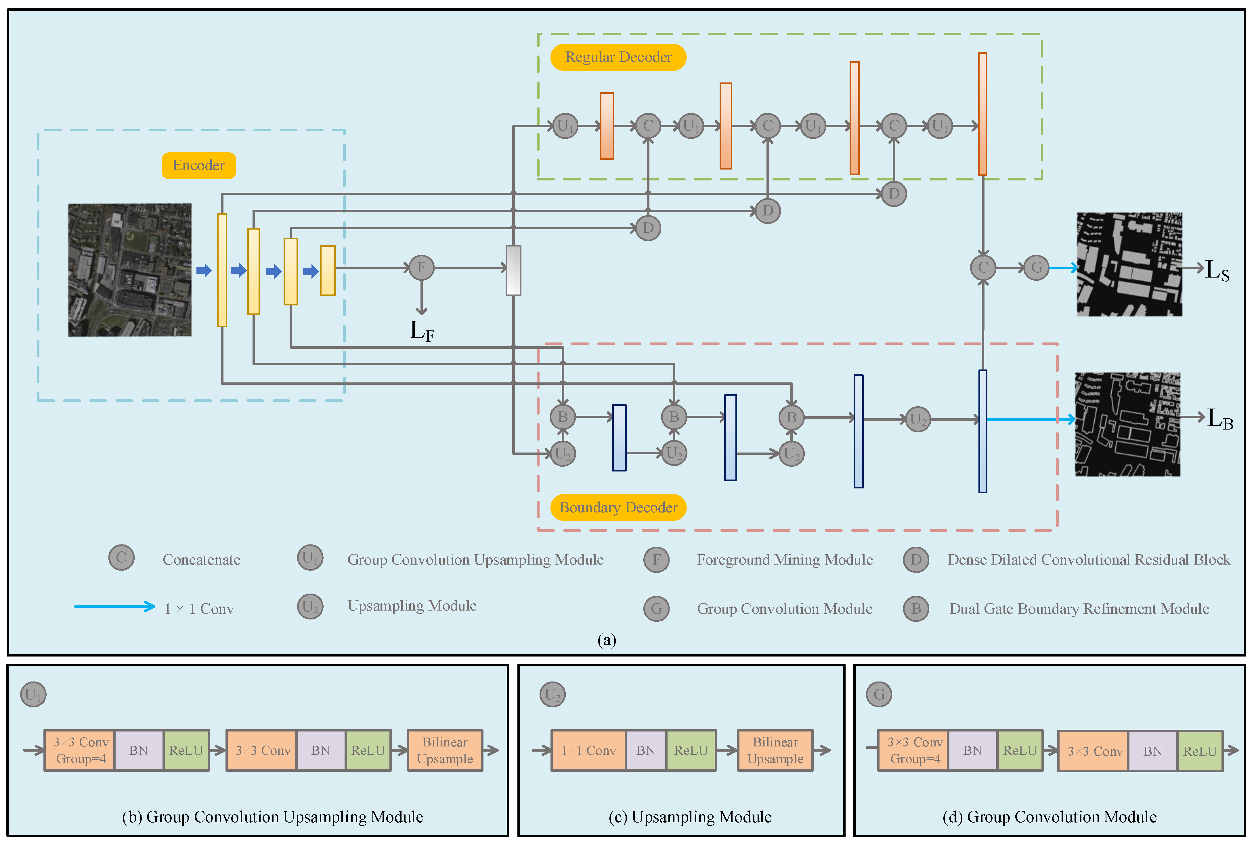
In order to solve the above two problems and improve the performance of building extraction, we propose a multi-task learning building extraction network in this paper. The main contributions are as follows:

(1)

The Foreground Mining Module (FMM) is proposed. A multi-scale relationship-based foreground modeling method is used to learn foreground features, including explicit modeling, sampling, and learning of foreground features, which can reduce model complexity while reducing background pixel interference;

(2)

The Dual Gate Boundary Refinement Module (DGBRM) and the Dense Dilated Convolutional Residual Block (DDCResBlock) are proposed to handle the boundary branch and the regular branch, respectively. DGBRM refines the boundary through spatial and channel gates. DDCResBlock efficiently extracts and integrates multi-scale semantic features from low-level feature maps, thereby expanding the receptive field of the feature maps;

(3)

We conducted experiments on two public datasets, the WHU Building Aerial Imagery Dataset and the Massachusetts Buildings Dataset. The ablation experiment has demonstrated the effectiveness of each module. The results of the comparative experiment indicate that our method outperforms the other compared methods in terms of performance while maintaining a relatively low computational complexity.

2. Related Work

2.1. Multi-Scale Features Extraction and Fusion

In the early field of computer vision, multi-scale images were mainly obtained through image pyramid transformation. Witkin et al. [29] introduced proportional space technology to generate coarser resolution images through Gaussian filters. This has attracted attention to the research of scale space methods. Lindeberg et al. [30] proposed a scale-normalized LoG (Laplacian of Gaussian) operator to handle changes in scale and solve the problem of previous work not having scale invariance. In recent years, deep learning-based methods have gradually replaced traditional methods in semantic segmentation. The most prominent among them is the FCN network, which replaces the fully connected layer with convolutional layers, allowing the model to accept images of any size, bringing the performance of semantic segmentation models to new heights. Afterward, networks derived from the FCN structure became the mainstream model in building extraction. The main improvement direction is the extraction and fusion of multi-scale features, which is conducive to improving the robustness of prediction results and producing more discriminative features. Panoptic SwiftNet [31] utilizes a multi-scale feature extraction and fusion method based on pyramid images for efficient panoramic segmentation. Sun et al. [32] proposed a high-resolution network architecture (HRNet), which effectively overcomes the loss of multi-scale information and achieves more accurate and robust feature learning by constructing a high-resolution feature pyramid network and feature fusion for cross resolution information interaction. In terms of feature fusion, Qiu et al. [33] proposed the AFL-Net, which introduced the attentional multiscale feature fusion (AMFF) module for multi-scale feature fusion. This approach abandons conventional concatenation or addition, opting instead to assign weights to pixels within each feature map by learning attention scores, subsequently enhancing the model’s performance. Ronneberger et al. [34] proposed a U-shaped structure network, which efficiently combines shallow local features with deep global features through skip connections. Afterward, numerous models were improved on the basis of U-Net. Zhou et al. [35] added denser skip connections in U-Net to reduce differences between encoder and decoder feature maps. Li et al. [36] proposed MANet, which designed kernel attention with linear complexity and applied it to the feature fusion stage of U-Net, improving performance with a lightweight structure. However, U-shaped structures often have limited receptive fields, and their decoders use a unified branch to fuse all features. In terms of feature extraction, many studies obtain multi-scale features and expand the receptive field through dilated convolutions or pooling modules with different structures. Zhao et al. [37] proposed PSPNet, which utilizes average pooling of different sizes to establish pyramid pooling module (PPM) to extract context at different scales. The DeepLab series [38,39] proposes the ASPP module to extract multi-scale features, which incorporates parallel dilated convolutions with different dilation rates. However, this type of method has a high computational complexity.

2.2. Enhancement of Foreground Features

The foreground–background imbalance stands as one of the most representative features in remote sensing imagery, and it is also an essential reason for the poor performance of a large number of natural image segmentation models applied to remote sensing images. To address this issue, current research mainly focuses on improving the loss function and model structure. In terms of the loss function, Lin et al. [40] proposed focal loss. It adds dynamic scaling factors on the basis of the binary cross-entropy loss to enhance the weight of indistinguishable samples in training, reduce the weight of distinguishable samples, and make the model focus on indistinguishable samples. Shrivastava et al. [41] proposed the Online Hard Example Mining (OHEM) loss, which sets samples with a probability of correct prediction below the threshold as difficult samples during each training iteration and only calculates the loss of difficult samples. In addition, loss functions such as dice loss [42] and weighted cross-entropy loss can also address this problem to some extent. In terms of model structure, Xu et al. [43] used an adaptive transformer fusion module to adaptively suppress noise, and further enhanced the saliency of the foreground through a detail-aware attention layer that includes spatial attention and channel attention. FarSeg [44] proposed a relationship-based foreground feature enhancement method, which utilizes the relationship between foreground pixels and the latent scene space to enhance foreground features and context. PFNet [45] addressed the issue of interference propagation during the feature map fusion process by independently fusing saliency points and boundary points from two feature maps. FactSeg [46] designed a dual decoder structure that activates small object foreground and suppresses large-scale background through foreground sensing branches and proposes a CP loss to effectively combine the predictions of the two branches, reducing training difficulty. Based on these studies, we optimized the process of foreground modeling and obtained multiscale latent scene space with stronger robustness and richer information. Based on the modeling, we improved the model’s ability to extract buildings of different styles by mining the connections between foreground and contextual features, reducing the interference of background features.

2.3. Boundary Refinement

Most current building extraction networks do not extract boundary features separately, resulting in blurred and imprecise segmentation results. Some studies [47,48,49,50] have also focused on boundary refinement. Wang et al. [51] proposed MEC-Net, which employed Sobel operators for extracting boundaries in the predictions and employed boundary labels to supervise the model, thereby enhancing the precision of boundaries. This type of method learns boundaries and other features in the same branch, but the features in remote sensing images are diverse, and learning distinct features in a single branch can lead to feature confusion and inefficiency in learning. Some studies [52,53,54,55,56] use a multi-branch structure to process different features. Xu et al. [53] added counter and distance branches on the basis of the conventional decoder, using feature maps of different scales to split different features and efficiently learn the boundary features. However, boundary branches are all learned through stacked convolution, lacking prior knowledge guidance. Guo et al. [54] and Lin et al. [55] both learned fine boundaries by decoupling semantic and edge, building body and edge, and further optimized the network by combining multi-objective loss functions to enhance the pertinence of edge feature extraction. Towaki et al. [56] proposed gated convolution based on the distribution of features, dividing shape and regular streams into two branches. Regular stream can help shape stream focus only on the boundary features. Shape stream helps the model recover boundary information. Based on this study, BFL-Net extends the gating mechanism to the decoding stage. Moreover, we simplify the spatial gate and add a channel gate. Accurate boundary features are extracted without the use of edge detection operators.

3. Materials and Methods

In this section, we will provide a detailed description of the proposed network. In Section 3.1, we will provide an overview of the overall structure of BFL-Net which is shown in Figure 1. In Section 3.2, Section 3.3 and Section 3.4, we detail the structures and design ideas of FMM, DDCResBlock, and DGBRM, respectively.

3.1. BFL-Net

We treat the building extraction task as a binary classification semantic segmentation problem. Our proposed BFL-Net is based on the classic encoder-decoder structure. Specifically, we adopt a multi-task learning strategy, using a U-shaped structure as the basic framework, ResNet50 as the encoder, and a dual-branch structure as the decoder. The two branches are used to complete boundary extraction and semantic segmentation tasks, respectively.

In the encoding process, we consider both predictive performance and efficient design. The output of ResNet50 generally contains five feature maps $Re{s}_k,k=\{1,2,3,4,5\}$ ($Re{s}_1$ is the output before the maxpool operation), where $k$ represents the downsampling, the ratio is $2^k$. In order to preserve the detailed features of remote sensing images and improve the segmentation ability of small buildings, we only use the first four feature maps $X_i\in {ℝ}^{C_i\times H_i\times W_i},i=\{1,2,3,4\}$, where $i$ represents the number of the feature map, $C_i$, $H_i$, and $W_i$ denote the channel, height, and width of the $i\mathrm{th}$ feature map output by ResNet50, respectively. Due to the interference of a large number of background pixels, the calculation of attention suffers negative impacts on both performance and efficiency. Therefore, $X_4$ is input into FMM to separate important foreground features, beneficial context and background features, and generate the foreground prediction. A detailed description of FMM can be found in Section 3.2.

In the decoding process, we design different decoding structures for the boundary and regular branch. For the boundary branch, a 1 × 1 convolution, batch normalization, ReLU activation function, and bilinear upsampling are used to compress channels and change the size of high-level feature maps to maintain consistency with low-level feature maps. High-level and low-level feature maps of the same size are input into DGBRM, reducing the semantic gap between the two feature maps while extracting rich boundary features from low-level feature maps in both spatial and channel dimensions. A detailed description of DGBRM can be found in Section 3.4. The final output of the boundary decoder is compressed in the channel dimension by a 1 × 1 convolution, obtaining a boundary prediction and learning boundary features through the supervision of the boundary label.

For the regular branch, $X_{1-3}$ contain rich low-level features, but due to insufficient receptive fields and the presence of numerous buildings exhibiting distinct characteristics or other objects sharing similar features with buildings, some low-level features may interfere with prediction due to their weak classification ability. Furthermore, in order to distinctively decode features, we aim for the regular decoder to focus on the features unrelated to boundaries. $X_{1-3}$ are input into DDCResBlock, which enhances the activation of high-level features by expanding the receptive field. The detailed structure of DDCResBlock is shown in Section 3.3. In terms of the fusion of low-level and high-level features, in order to reduce computational complexity, we abandoned the decoding method in U-Net. Instead, a 3 × 3 group convolution with 4 groups, batch normalization, and ReLU activation function are used to adjust the channel dimension, a 3 × 3 convolution, batch normalization, and ReLU activation function are used for feature fusion, and bilinear upsampling is used to increase the size of the feature map. Ultimately, a feature map of the same size as the low-level feature map of the previous layer is obtained. In the fusion stage, after concatenating the outputs of the two branches, the channel dimension is reduced to 16 through the Group Convolution Module. Finally, a 1 × 1 convolution is used to obtain the building prediction.

3.2. Foreground Mining Module (FMM)

In order to complete the learning of foreground features with less interference from background information, we designed a Foreground Mining Module (FMM) to independently learn foreground features, as shown in Figure 2. This module mainly consists of four parts: foreground modeling, sampling, learning, and fusion. The specific implementation method is as follows: In order to reduce computational complexity and align features into a shared manifold for subsequent similarity calculations, for the input feature map $X_4\in {ℝ}^{C_4\times H_4\times W_4}$, the channel dimension is compressed to $C_4/4$ through a projection function $\omega (\cdot )$, which is implemented through a 1 × 1 convolution, batch normalization, and ReLU activation function, resulting in $X_4^{\ast }\in {ℝ}^{C_4/4\times H_4\times W_4}$.

In the modeling stage, buildings can be roughly divided into residential buildings, public buildings, industrial buildings, and agricultural buildings in terms of functionality. Each type of building exhibits significant intra-class consistency and inter-class differences in features such as size, shape, and texture. In urban planning, buildings typically exhibit regional consistency, which means that buildings of the same category and with similar features often tend to cluster in the same region. Based on the above prior knowledge, inspired by FarSeg, the high correlations existing between foreground semantics, contextual semantics, and the latent scene space are used to design a Foreground Mining Module (FMM). Specifically, as shown in Figure 3, the latent scene space locates foreground features and important contextual features through high correlations, and contextual features can enhance the expression of foreground features in learning. To prevent inaccurate foreground extraction caused by background pixels dominating the scene space, unlike the 1-d latent scene space obtained through global pooling in FarSeg, we utilize multiple sets of asymmetric depthwise large kernel convolutions and global average pooling (GAP) operation to perceive scene space within the region at different scales. Subsequently, the projection function $\eta ()$ is used to learn the importance of multi-scale latent spaces in each region and align features to the same manifold as $X_4^{\ast }$, resulting in a 3-D scene space $X_4^s\in {ℝ}^{C_4/4\times H_4\times W_4}$. Compared to the 1-D scene space in FarSeg, each vector in $X_4^s$ contains scene space features of different regions and scales, which has stronger robustness. The process is formulated as Equations (1) and (2):

$${X^{\prime }}_4=f_{5\times 5DWSConv}(X_4^{})$$

(1)

$$X_4^s=\eta (Concat({\phi }_7({X^{\prime }}_4),{\phi }_{11}({X^{\prime }}_4),{\phi }_{21}({X^{\prime }}_4),f_{UP}(f_{GAP}({X^{\prime }}_4)),{X^{\prime }}_4))$$

(2)

where $f_{5\times 5DWSConv}()$ is a 5 × 5 depthwise separable convolution, ${\phi }_i()$ represents a set of depthwise asymmetric convolutions, i means the size of the convolution kernel, $f_{GAP}()$ is global average pooling, $f_{UP}()$ represents the bilinear upsampling, $Concat()$ denotes the concatenate operation, and $\eta ()$ represents a projection function used to generate scene features which is implemented through a 1 × 1 convolution, batch normalization and ReLU activation function.

In order to localize foreground and beneficial contextual pixels by computing the correlation between each feature vector in $X_4^s$ and the corresponding vector in $X_4^{\ast }$, from an efficient perspective, inner product similarity is used as the calculation method, resulting in the probability map $S\in {ℝ}^{1\times H_4\times W_4}$. In order to separate foreground pixels and beneficial context, we sparsely sample $X_4^{}$ using the probability map $S$. Because sparse sampling can disrupt the positional relationship of feature vectors, we need to perform position encoding before sampling. Many studies [57,58,59] have found that introducing zero padding in convolutional operations can encode absolute position information. We use a function $\lambda ()$ for position encoding, resulting in $X^e$. Then, the $k$ pixels with the highest score in $S$ are selected and their position index is $I\in {ℝ}^{k\times 2}$. Then, $T$ is obtained by sampling $X^e$ through $I$. The sampled sparse vectors can effectively represent foreground features and important context. The process is formulated as Equations (3)–(5):

$$X^e=\lambda (X_4)+X_4$$

(3)

$$I=topk(S,k)$$

(4)

$$T=gather(X^e,I)$$

(5)

where $\lambda ()$ represents a position encoding function implemented by a 3 × 3 depthwise convolution, $topk(S,k)$ represents the 2-D coordinate indices of the $topk$ maximum values output from $S$ and $gather(\ast ,I)$ represents obtaining the 2-D tokens corresponding to the position of the 2-D coordinate index $I$ from the complete feature map.

In the learning stage, the sampled tokens are learned by establishing global connections through the kernel attention mechanism (KAM) [36]. KAM is an efficient attention mechanism. For query $Q$, key $K$, and value $V$, in the dot-product attention, the similarity between the $i\mathrm{th}$ query feature and the $j\mathrm{th}$ key feature is calculated using the softmax normalization function through $e^{q_i{k}_j}$, where $q_i$ and $k_j$ denote the $i\mathrm{th}$ query feature and the $j\mathrm{th}$ key feature, respectively. KAM uses two softplus functions acting on $q_i$ and $k_j$ as kernel smoothers instead of the original similarity calculation method, transforming complexity from $O(N^2)$ to $O(N)$. The simplified calculation method is shown in Equation (6).

$$D{\left(Q,K,V\right)}_i=\frac{softplus{(q_i)}^T{\displaystyle {\sum }_{j=1}^{N}softplus(k_j)v_j^T}}{softplus{(q_i)}^T{\displaystyle {\sum }_{j=1}^{N}softplus(k_j)}}$$

(6)

where $D{(Q,K,V)}_i$ represents the attention score between the $i\mathrm{th}$ query feature and the $j\mathrm{th}$ key feature, $N$ means the number of sampled tokens, $softplus()$ is the softplus activation, and ${(\cdot )}^T$ denotes the transpose operation.

In the fusion stage, for the purpose of facilitating training, we employ residual structures to fuse features, resulting in $T^{\prime }$. Finally, employing $I$, we scatter $T^{\prime }$ into $X_4$, obtaining a more enriched and refined foreground feature $X_4^f$. The process is formulated as Equations (7) and (8):

$$T^{\prime }=Attention(T)+T$$

(7)

$$X_4^f=Scatter(X_4^e,T^{\prime },I)$$

(8)

where $Attention()$ represents using the KAM module to process input tokens, resulting in higher semantic tokens and $Scatter(X_4^e,T^{\prime },I)$ denotes scattering $T^{\prime }$ into the $X_4^e$ according the index $I$.

3.3. Dense Dilated Convolutional Residual Block (DDCResBlock)

In order to achieve distinctive feature fusion and focus regular branch on the fusion of high-level features, DDCResBlock is designed to expand the receptive field and enhance the classification ability of low-level features. The specific structure is shown in Figure 4. DDCResBlock enhances the perception of multi-scale features through dilated convolutions with different dilation rates, which is beneficial for capturing features of buildings with significant scale variations.

The specific implementation method is as follows: The outputs of the backbone $X_{\mathrm{i}},i=\{1,2,3\}$ are input into the residual structure, as shown in Figure 4. In the first step, a 1 × 1 convolution is used to establish the propagation of information between channels, facilitating subsequent feature map splitting. Then, the feature map is uniformly divided into four parts along the channel dimension, resulting in $F_i,i=\{1,2,3,4\}$ which learns multi-scale features through a dense dilated convolution structure. Specifically, global semantic information ${F^{\prime }}_4$ is obtained from $F_4$ through global average pooling and upsampling. Multi-scale features are obtained from $F_{1-3}$ through the densely cascaded Asymmetric Separable Convolution Block (ASCB), which can be formulated as Equations (9) and (10):

$${F^{\prime }}_1=A(F_1)$$

(9)

$${F^{\prime }}_i=A({F^{\prime }}_{i-1}+F_i),i=\{2,3\}$$

(10)

where $A()$ represents ASCB, ${F^{\prime }}_i$ is the output of ASCB applied to the input $F_i$.

The dense cascade structure fully utilizes the advantages of residual structure in model learning and feature propagation. Based on expanding receptive fields through dilated convolution, the dense cascade structure can not only obtain more dense and continuous feature representations but also provide a broader range of receptive field scales. In order to achieve a better balance between efficiency and performance, ASCB is inspired by dilated convolution, asymmetric convolution, and depthwise separable convolution. 1 × 3 and 3 × 1 depthwise separable convolutions with a dilation rate of $r$ are used to expand the receptive field of the feature map at a low cost. Then, a 1 × 1 pointwise convolution is used for weighted fusion along the channel dimension. In order to avoid the gridding effect of dilated convolution, the dilation rates of dilated convolutions are set to 1, 3, and 9, respectively, according to the principle proposed by Wang et al. [60]. Finally, we concatenate ${F^{\prime }}_{1-4}$ and obtain the output through channel attention and residual connection. Overall, compared to traditional ResBlock, DDCResBlock can fuse multi-scale features and have a larger receptive field. Compared to the ASPP module, it offers a more lightweight architecture with a smoother continuous receptive field and a richer scale.

3.4. Dual Gate Boundary Refinement Module (DGBRM)

Remote sensing images contain low-level features such as boundary and texture, as well as high-level semantic features. Among low-level features, boundary feature provides more structural information and is considered higher-level features compared to pixel-level features. Based on the above prior knowledge, it is reasonable to use high-level feature maps to guide low-level feature maps to activate features related to boundaries and reduce interference from other features. To address the issue of easily losing boundary details during the upsampling process, we divide the upsampling process into regular and boundary streams and introduce the DGBRM in each fusion process of the boundary stream. In the early stage, the boundary stream focuses on low-level features. After introducing high-level features through DGBRM, spatial and channel gates assist boundary stream in filtering out noise features, retaining features related to the boundary for boundary extraction.

The gating mechanism is equivalent to a regulating valve, which can regulate the degree of incoming information flow and is a commonly used method of filtering information. Using the gating mechanism during the decoding phase can not only extract boundary features but also reduce the semantic gap between feature maps in feature fusion. Takikawa et al. [56] proposed GSCNN, which was the first to utilize gating mechanisms to extract boundary features. Inspired by GSCNN, DGBRM is designed to extract boundary features, as shown in Figure 5. We extend the gating mechanism to the decoding stage and perform feature filtering through simple spatial and channel gates. Accurate boundary features are extracted without the use of edge detection operators.

DGBRM mainly includes the spatial gate and the channel gate. For the input low-level feature map $X_i$ and high-level feature map $X_{i+1}^{in}\in {ℝ}^{C_i\times H_i\times W_i}$ which is obtained by upsampling $X_{i+1}^b$ and compressing it in the channel dimension through Upsampling Module, we concatenate them for generating gates. In the channel gate, a 1 × 1 convolution, batch normalization and ReLU activation function are employed for feature fusion. Then, GAP is used to compress features on the spatial dimension, and a 1-d convolution is used to interact between adjacent channels. Finally, we obtain the channel gate $c_i\in {ℝ}^{C_i\times 1\times 1}$ through the sigmoid activation. In the spatial gate, we simply compress the channel dimension through a 1 × 1 convolution, batch normalization, and ReLU activation. Subsequently, the sigmoid activation is used to generate a spatial gate $s_i\in {ℝ}^{1\times H_i\times W_i}$. Finally, the low-level feature map is sequentially multiplied by the channel and spatial gates to obtain the boundary feature $X_i^b\in {ℝ}^{C_i\times H_i\times W_i}$. The process can be formulated as Equations (11)–(13):

$$c_i=\sigma (f_{Conv1d}(f_{GAP}(f_{Conv2d}(Concat(X_i,X_{i+1}^{in})))))$$

(11)

$$s_i=\sigma (f_{Conv2d}(Concat(X_i,X_{i+1}^{in})))$$

(12)

$$X_i^b=f_S(s_i,f_C(c_i,X_i))$$

(13)

where $Concat()$ represents the concatenate operation, $f_{Conv2d}()$ means the 1 × 1 2-d convolution layer, $f_{Conv1d}()$ is the 1-d convolution with a kernel size of 5, $\sigma ()$ denotes the sigmoid activation, $f_C()$ represents the multiplication in the channel dimension, and $f_S()$ represents the multiplication in the spatial dimension.

3.5. Loss Functions

3.5.1. Semantic Segmentation Loss

To solve the imbalance problem in building extraction, we use the OHEM strategy to calculate the segmentation loss $L_S$. It can focus on difficult samples during training. Specifically, we rank the correct prediction probability of each pixel from low to high and obtain $C\in {ℝ}^{N\times 1}$ where $N$ represents the total number of pixels. Next, pixels with a probability lower than the threshold we set are selected as difficult samples. Finally, when calculating cross-entropy loss (CE loss), only the difficult sample loss is calculated, ignoring the easy sample loss.

3.5.2. Boundary Loss

There is also a class imbalance issue with boundaries. However, considering the convergence speed of the model and the performance of boundary extraction, we use dice loss to calculate the boundary loss $L_B$.

3.5.3. Foreground Loss

Although there is also an imbalance problem with foreground samples, in foreground prediction, only rough positioning of the foreground is required without fine segmentation and classification. Therefore, in order to reduce the difficulty of model training, the binary cross-entropy loss (BCE loss) is used to calculate the foreground loss $L_F$.

In summary, the final loss $L$ is defined as Equation (14):

$$L={\alpha }_1{L}_S+{\alpha }_2{L}_B+{\alpha }_3{L}_F$$

(14)

where ${\alpha }_1$, ${\alpha }_2$, ${\alpha }_3$ represents the weight of each loss.

4. Results and Analysis

4.1. Datasets

The WHU Building Aerial Imagery Dataset includes satellite datasets and aerial image datasets, with a spatial resolution of 0.3 m–2.5 m. We only conducted experiments on the aerial image dataset, which was mainly filmed from Christchurch, New Zealand, covering 220,000 buildings of various forms with a coverage area of 450 ${\mathrm{km}}^2$.

The Massachusetts Building dataset was mainly captured in the urban and suburban areas of Boston, USA, with a spatial resolution of 1 m. Each image covers 2.25 ${\mathrm{km}}^2$, and all images cover approximately 350 ${\mathrm{km}}^2$.

4.2. Data Preprocessing

Before the experiment, we preprocessed both datasets. We set the pixel with the semantic meaning of building in the label to 1 and the pixel with the semantic meaning of background to 0 as the segmentation label and foreground label and used the findContours function in OpenCV to obtain the boundary label of the image. WHU Building dataset images have a size of 512 × 512 pixels, and the training set, validation set, and test set have been divided. We will not perform any operations. Massachusetts Building dataset images have a size of 1500 × 1500 pixels. We cropped the original image to 512 × 512 pixels, with an overlap of 256 pixels. Each image has been divided into 25 images. Due to the presence of a large number of blank pixels in some images, we removed them for training efficiency. The divisions of the processed dataset are listed in

Table 1. The divisions of each dataset.

Dataset	Training Set (Tiles)	Validation Set (Tiles)	Test Set (Tiles)
WHU dataset	4736	1036	2416
Massachusetts dataset	3289	100	250

.

4.3. Evaluation Metrics

In this paper, we use four commonly used metrics for semantic segmentation: Intersection over Union (IoU), F1-score, Recall, and Precision to evaluate the performance of building extraction. IoU is the ratio of the intersection and union of pixels predicted as buildings and pixels labeled as buildings. Recall reflects the model’s recognition ability for positive samples, Precision reflects the model’s recognition ability for negative samples, and F1-score is the harmonic average of Recall and Precision, which is a comprehensive reflection of Recall and Precision. The calculation formulas are as follows:

$$\mathrm{IoU}=\frac{\mathrm{TP}}{\mathrm{FN}+\mathrm{TP}+\mathrm{FP}}$$

(15)

$$\mathrm{Recall}=\frac{\mathrm{TP}}{\mathrm{FN}+\mathrm{TP}}$$

(16)

$$\mathrm{Precision}=\frac{\mathrm{TP}}{\mathrm{FP}+\mathrm{TP}}$$

(17)

$$\mathrm{F}1-\mathrm{score}=\frac{2\times \mathrm{Precison}\times \mathrm{Recall}}{\mathrm{Precision}+\mathrm{Recall}}$$

(18)

where TP, FP, TN, and FN represent true positive samples, false positive samples, true negative samples, and false negative samples, respectively.

4.4. Experimental Settings

In this paper, all models were implemented based on Python-3.8 and PyTorch-1.11.0, and all experiments were conducted on a single Nvidia GeForce RTX 3090 GPU. L2 regularization and data augmentation methods, including random horizontal flipping, random vertical flipping, random rotation, and random Gaussian blur, were used to avoid overfitting. During training, we used the Adam optimizer with an initial learning rate of 0.0005, and the Poly learning rate was used to decay the learning rate. The batch size was set to 12. In the WHU dataset and the Massachusetts dataset, the number of epochs is set to 200 and 300, respectively.

4.5. Comparative Experiments

4.5.1. Introduction of the Models for Comparison

We compare our proposed model with state-of-the-art models to demonstrate the advancement of our model. The comparison model selection process is as follows: because the overall structure of our model is based on a U-shaped structure, U-Net++ is chosen as the comparison. HRNet is the classic model in natural image segmentation, which have been widely used in research and industry. FarSeg, PFNet, and FactSeg are models that have achieved significant results in remote sensing image segmentation in recent years. They can solve the imbalance problem in tasks such as building extraction to a certain extent. MANet improves the problem of insufficient information utilization in feature fusion of U-Net through a linear complexity of attention, achieving state-of-the-art performance in multiple remote sensing image datasets. STT, AFL-Net, and MEC-Net are models that have achieved significant results in building extraction from remote sensing images in recent years.

4.5.2. Comparisons with State-of-the-Art Methods

For all methods, official codes were used for experimentation. Due to the lack of code provided by AFL-Net, we implemented the code based on the original paper.

The results of the comparative experiments on the WHU dataset and the Massachusetts dataset are shown in

Table 2. Results of different models on the WHU dataset and Massachusetts dataset.

Model	WHU Dataset				Massachusetts Dataset
	IoU (%)	Precision (%)	Recall (%)	F1 (%)	IoU (%)	Precision (%)	Recall (%)	F1 (%)
PFNet [45] (2021)	89.98	95.63	93.84	94.73	72.79	86.71	81.94	84.26
MANet [36] (2021)	89.09	93.62	94.86	94.24	72.07	86.21	81.46	83.38
FarSeg [44] (2020)	90.06	95.47	94.08	94.77	72.74	87.34	81.31	84.22
U-Net++ [35] (2018)	89.19	94.96	93.62	94.29	71.03	85.14	81.09	83.07
FactSeg [46] (2022)	90.56	95.24	94.23	95.05	73.69	87.37	82.48	84.85
HRNet [32] (2019)	89.86	95.38	93.95	94.66	72.01	87.08	80.62	83.73
STT [27] (2021)	90.29	95.46	94.34	94.90	71.86	81.34	83.63	84.56
AFL-Net [33] (2022)	90.82	95.24	95.15	95.19	73.27	85.23	83.92	84.57
MEC-Net [51] (2023)	90.67	94.62	95.60	95.11	73.89	81.99	88.20	84.98
BFL-Net (Ours)	91.37	96.04	94.95	95.49	74.50	88.20	82.76	85.39

Note: The best result is represented in bold.

. On the WHU dataset, our model achieved the best in IoU, Precision, and F1-score, with improvements of 0.55%, 0.41%, and 0.3% compared to the second-ranked model, respectively. MEC-Net achieved the best in Recall, surpassing the second-ranked model by 0.45%. On the Massachusetts dataset, our model achieved the best in IoU, Precision, and F1-score, with improvements of 0.61%, 0.83%, and 0.41% compared to the second-ranked model, respectively. MEC-Net achieved the best in Recall, surpassing the second-ranked model by 4.28%. Overall, our model achieved the best results on both datasets. This fully demonstrates the effectiveness of our model. In addition, models optimized for the imbalance of foreground and background in remote sensing images, such as FarSeg and PFNet, as well as FactSeg and BFL-Net, achieved stable performance on both datasets by reducing background interference. In addition, networks specifically designed for extracting buildings from remote sensing images, such as AFL-Net and MEC-Net, also perform well. On the contrary, some networks used for natural image segmentation or multi-class semantic segmentation of remote sensing images, such as MANet and U-Net++, have achieved poor performance on one or two datasets. Therefore, not all semantic segmentation models are suitable for building extraction tasks. Finally, it is worth noting that our proposed BFL-Net outperforms other models in terms of Precision on both datasets and is higher than Recall by 1.09% and 5.44%, respectively. The reason may be that BFL-Net has explicitly modeled and independently learned foreground features, thereby reducing the interference of background features of suspected buildings, reducing misjudgment to a certain extent, and making a significant contribution to Precision, making it very suitable for tasks with high Precision requirements.

4.5.3. Comparison of Different Foreground Modeling Methods

As shown in Figure 6, we compared four foreground modeling methods. (a) [27] and (b) [45] are convolution-based methods, while (c) [44] and (d) are relationship-based methods. Foreground-Recall (F-Recall) and IoU are employed as evaluation metrics in this experiment. F-Recall is used to measure the performance of methods in foreground localization, while IoU is used to measure the contribution of the method to the final prediction result. For F-Precision, we set the 256 points with the highest score in the foreground modeling stage to 1 and the remaining points to 0. After nearest upsampling, the Recall is calculated from the foreground predictions and the foreground labels. The IoU is calculated from final predictions and building labels.

Table 3. Results of different modeling methods on the WHU dataset and Massachusetts dataset.

Method	WHU Dataset		Massachusetts Dataset
	F-Recall (%)	IoU (%)	F-Recall (%)	IoU (%)
(a)	87.53	90.97	67.81	73.58
(b)	87.06	90.82	66.98	73.42
(c)	87.92	91.18	68.02	73.95
(d) (Ours)	88.57	91.37	68.85	74.50

Note: The best result is represented in bold.

shows a comparison of different mainstream foreground modeling methods. The results show that relationship-based methods are superior to convolution-based methods, and our foreground modeling method achieves the best performance in both F-Recall and IoU metrics, which proves that FMM can not only locate the foreground position in the middle of learning, but also bring positive improvements to the final prediction results by enhancing foreground and beneficial context. It is worth noting that all foreground modeling methods do not perform well in F-Recall on the Massachusetts dataset. The reason is that the buildings in the Massachusetts dataset are small and dense, and the features in the foreground modeling stage lack the integration of low-level features, which leads to only rough positioning of these buildings.

4.5.4. Visualization of Experimental Results

To more intuitively reflect the performance of each model, we visualized their building prediction results on the WHU dataset and Massachusetts dataset. The two datasets have buildings of different styles and densities. Specifically, the buildings on the WHU dataset are larger and more dispersed, and the buildings on the Massachusetts dataset are smaller and denser. The visualization results on both datasets can fully reflect the model’s ability to extract architectural clusters of different styles. We selected four representative images on each of the two datasets.

The visualization results of each model on the WHU dataset are shown in Figure 7. Overall, our proposed BFL-Net has fewer pixels for incorrect prediction and is visually superior to other models. Specifically, in (a) $①$, due to the small and dense buildings, all models had missed extractions. However, BFL-Net had the fewest pixels of false extractions, with only a few pixels being overlooked. In (a) $②$, only BFL-Net, FarSeg, and U-Net++ accurately predicted boundaries because the color of the edges on the right side of the building was different from the overall color. The above results indicate that BFL-Net has better predictive ability in building details, boundaries, and easily overlooked small buildings. In (d) $③$, in the prediction of large buildings, U-Net++, MANet, STT, MEC-Net, PFNet, and AFL-Net all showed a large number of missed pixels inside the building, possibly due to changes in the texture inside the large building and the model could not effectively recognize as the same building. HRNet showed a small number of missed pixels inside the building. FarSeg does not predict smoothly and accurately on the right boundary, while BFL-Net predicts more accurately on both internal pixels and boundaries. However, it is also noteworthy that all models generated numerous incorrect predictions in the areas marked within the red circles in the image. This might be attributed to certain angles in the capture, causing an inclination in the imaging of buildings, thereby resulting in false predictions. Overall, the above results indicate that BFL-Net can predict large buildings more accurately and stably through large receptive fields and multi-scale perception, with fewer missed detections inside buildings.

The visualization results of each model on the Massachusetts dataset are shown in Figure 8. Overall, our proposed BFL-Net outperforms other models visually. Specifically, in (b) $①$, the five buildings are small and scattered. Only BFL-Net, U-Net++, FactSeg, MEC-Net, PFNet, and AFL-Net accurately predicted five buildings. The above results indicate that BFL-Net can predict details in images more accurately by utilizing low-level features reasonably. In (c) $②$, except for BFL-Net, all models had missed detections inside the building, and BFL-Net almost perfectly predicted the building, indicating that BFL-Net improved the prediction ability inside the building through multi-scale receptive fields. However, it is worth noting that the presence of densely distributed buildings with considerable background clutter (as shown in the red circle area in Figure 8b) or complex structures on building rooftops (as shown in the red circle area in Figure 8c) can result in the occurrence of shadows and occlusions. Shadows and occlusions in remote sensing images are critical factors that affect the performance of building extraction.

The visualization results of various models on the WHU dataset and Massachusetts dataset indicate that BFL-Net has advantages in predicting building details, small buildings, and internal pixels of large buildings, and the model has strong robustness and is not easily affected by factors such as building textures.

To verify the effectiveness of FMM in foreground prediction, we visualized the sampling points in foreground prediction. Specifically, we will represent the sampled points in white and the unsampled points in black. To improve visualization quality, we upsampled the prediction results to a size of 512 × 512 using the nearest-neighbor interpolation method. The visualization results on the WHU dataset and the Massachusetts dataset are shown in Figure 9 and Figure 10, respectively. The visualization results indicate that FMM can relatively accurately locate foreground pixels in the mid-term of model learning. In addition, for small buildings that are difficult to extract, FMM can also enhance the expression of these features by locating their relevant important contexts.

4.5.5. Comparison of Complexity

The WHU dataset is a widely used and highly accurate dataset for building extraction in remote sensing images. Therefore, we use the results of the model on the WHU dataset as a basis for measuring the model’s ability to extract buildings in this section. The IoU, the number of parameters (Params), and the floating-point operations (FLOPs) are used as evaluation metrics. IoU is an evaluation metric used to evaluate the performance of model predictions. The higher the IoU, the more accurately the model can extract buildings. Params and FLOPs are metrics for evaluating model complexity, and lower Params and FLOPs demonstrate that the model is lighter and more conducive to practical applications. All metrics were computed using code either open-sourced by the authors or code implemented by us.

The comparison of IoU, Params, and FLOPs of each model is shown in Figure 11 and Figure 12. Each dot represents the performance of a model on evaluation metrics, and the larger the diameter of the circle, the larger the Params or FLOPs of the model. Our proposed BFL-Net achieved the best performance on IoU, surpassing the second-place AFL-Net by 0.55%. On Params, our model has the second smallest Params among all comparative models, only 17.96 M. On FLOPs, our model ranks third smallest FLOPs among all comparative models, with only 50.53 G. Overall, BFL-Net achieved a better balance between efficiency and performance.

4.6. Ablation Study

4.6.1. Ablation on Each Module

To verify the effectiveness of the proposed module in this paper, we split and combine modules for verification. We conducted experiments on the WHU dataset and the Massachusetts dataset. First, we use a dual decoder structure similar to FactSeg as the baseline. Specifically, we have replaced the feature fusion and upsampling modules in the decoding process of FactSeg with the same structure as BFL-Net. We have modified the foreground branch of FactSeg to a boundary prediction branch and added a feature fusion module in BFL-Net to fuse the features of the two branches. Next, we added the Foreground Mining Module (F), Dense Dilated Convolutional Residual Block (D), spatial gate (S), and channel gate (C) in the Dual Gate Boundary Refinement Module on the baseline to verify the effectiveness of each module. Finally, all modules were integrated together to verify the overall effectiveness of the model.

The experimental results on the WHU dataset are shown in

Table 4. The results of the ablation experiments of the BFL-Net on the WHU dataset.

Method	F	D	S	C	IoU (%)	Precision (%)	Recall (%)	F1 (%)	Increase in IoU (%)
Baseline	-	-	-	-	87.96	93.20	94.00	93.60	+0
Baseline + F	√	-	-	-	89.97	95.37	94.09	94.72	+2.01
Baseline + FD	√	√	-	-	90.76	95.92	94.41	95.16	+2.80
Baseline + FDS	√	√	√	-	91.15	95.91	94.83	95.37	+3.19
Baseline + FDC	√	√	-	√	91.05	96.02	94.62	95.32	+3.09
Baseline + FDSC	√	√	√	√	91.37	96.04	94.95	95.49	+3.41

Note: The best result is represented in bold.

, which can fully demonstrate the effectiveness of each module. Firstly, we used FactSeg with Resnet 50 (R₄) as the baseline for the experiment, with an IoU of 87.96%. Then, we added FMM on the baseline, and the IoU increased by 2.01% to 89.97%. It is worth noting that the addition of FMM has a significant improvement in Precision, with a 2.17% increase compared to baseline, indicating that FMM can effectively enhance the expression of foreground information through foreground learning, reduce misjudgment caused by background pixel interference, and improve Precision. Next, we added DDCResBlock, which increased IoU by 2.80% compared to baseline and 0.79% compared to “Baseline + F”. This indicates that DDCResBlock can increase the model’s perception of large buildings by expanding the receptive field, thereby improving performance. Then, we added spatial gate and channel gate, respectively, with IoU increasing by 3.19% and 3.09% compared to baseline and 0.39% and 0.29%, respectively, compared to “Baseline + FD”. This indicates the necessity of adding gates in both spatial and channel dimensions, which can help the model more comprehensively separate and restore boundary information. Finally, we added FMM, DDCResBlock, and DGBRM together to the baseline, resulting in an IoU increase of 0.22% and 0.32%, respectively, compared to “Baseline + FDS” and “Baseline + FDC”. The above experiments fully demonstrate that each module is effective while combining them not only does not create conflicts but also has positive effects. The above results indicate that using all modules together in our model achieves optimal performance.

The effectiveness of each module was once again verified through the experimental results of the model on the Massachusetts dataset in

Table 5. The results of the ablation experiments of the BFL-Net on the Massachusetts dataset.

Method	F	D	S	C	IoU (%)	Precision (%)	Recall (%)	F1 (%)	Increase in IoU (%)
Baseline	-	-	-	-	69.25	84.48	79.35	81.83	+0
Baseline + F	√	-	-	-	72.34	86.59	81.47	83.95	+3.09
Baseline + FD	√	√	-	-	73.19	87.18	82.02	84.52	+3.94
Baseline + FDS	√	√	√	-	73.92	87.03	83.08	85.01	+4.67
Baseline + FDC	√	√	-	√	73.80	86.85	83.02	84.90	+4.55
Baseline + FDSC	√	√	√	√	74.50	88.20	82.76	85.39	+5.25

Note: The best result is represented in bold.

. The addition of F, D, S, and C resulted in improvements of 3.09%, 0.85%, 0.73%, and 0.61% on IoU, respectively. The incorporation of all four modules together has increased by 5.25%, 3.72%, 3.41%, and 3.56% compared to baseline on IoU, Precision, Recall, and F1-Score, respectively.

To verify that our proposed DGBRM can effectively extract boundary information, we evaluated the results of the above ablation experiments using the Boundary IoU [61] as an evaluation metric, as shown in Figure 13. On the WHU dataset, compared to the baseline, the boundary IoU of each group showed varying degrees of improvement, with the most significant improvement being the “Baseline + F” group. We analyzed the reason for this because the structure of the baseline was too simple, and the receptive field was small. FMM not only expanded the receptive field to a certain extent but also allowed the model to learn diverse foreground features, which enabled numerous unrecognizable buildings to be identified. Even if the boundaries are not precise and fine enough, it also enhances the Boundary IoU. In addition, the modules that contribute the most to the boundary IoU are SC, S, C, and D in order. Especially based on improving the receptive field and being able to comprehensively learn building features through “Baseline + FD,” SC still increased the Boundary IoU by 1.61%, indicating that boundary details have indeed been refined. Then, the results of “Baseline + FDS” and “Baseline + FDC” indicate that both spatial gate and channel gate contribute to the improvement in boundary IoU. The situation in the Massachusetts dataset is similar to that in the WHU dataset, where the spatial gate and channel gate respectively increase Boundary IoU by 1.35% and 1.17% compared to “Baseline + FD”, and the combined use of the two modules increases Boundary IoU by 2.32%.

4.6.2. Ablation on Different Backbones

We compared the effects of different backbones on the experimental results. The notations used in the following experiments are described as follows:

• R₄: Using $Re{s}_{1-4}$ as the backbone;
• R₅: Using $Re{s}_{1-5}$ as the backbone.

As shown in

Table 6. Results of BFL-Net with different backbones on the WHU and Massachusetts datasets.

Backbone	WHU Dataset				Massachusetts Dataset
	IoU (%)	Precision (%)	Recall (%)	F1 (%)	IoU (%)	Precision (%)	Recall (%)	F1 (%)
ResNet18(R4)	90.38	95.60	94.30	94.95	72.80	87.03	81.66	84.26
ResNet18(R5)	90.34	95.46	94.40	94.93	72.65	86.82	81.65	84.16
ResNet50(R4) (Ours)	91.37	96.04	94.95	95.49	74.50	88.20	82.76	85.39
ResNet50(R5)	91.35	96.02	94.94	95.48	74.22	86.28	84.16	85.20

Note: R₄: Using $Re{s}_{1-4}$ as the backbone. R₅: Using $Re{s}_{1-5}$ as the backbone. The best result is represented in bold.

, on the WHU dataset, the proposed BFL-Net with ResNet50 (R₄) achieved the best performance across all metrics. On the Massachusetts dataset, BFL-Net with ResNet50 (R₄) performed the best in IoU, Precision, and F1-score, while BFL-Net with ResNet50 (R₅) achieved the best in Recall. Overall, using ResNet50 as the Backbone outperforms ResNet18 because ResNet50 uses more ResBlocks and has stronger feature extraction ability. BFL-Net with ResNet50 (R₄) is better than ResNet50 (R₅). The reasons can be listed as follows: (i) ResNet50 (R₄) has higher resolution, preserves more detailed features, and is more conducive to extracting dense small buildings. (ii) ResNet50 (R₅) has advantages in receptive fields and large-scale building extraction. However, the advantage is weakened due to the capture of global contextual information through KAM after the backbone and may be overfitting due to a large number of parameters.

4.6.3. Ablation on Dilated Convolutions with Different Structures

As shown in Figure 4 and Figure 14, we compared three different structures of ASCB in DDCResBlock: serial, parallel, and dense cascade structures. Note that in the experiment, we only changed the cascade structure of ASCB in DDCResBlock, and the rest of the structures remained consistent. As shown in

Table 7. Results of ASCB with different structures on the WHU and Massachusetts datasets.

Structure	WHU Dataset	Massachusetts Dataset
	IoU (%)	IoU (%)
Series	91.27	74.37
Parallel	91.23	74.29
Dense cascade (Ours)	91.37	74.50

Note: The best result is represented in bold.

, the performance of the dense cascade structure on both the WHU dataset and the Massachusetts dataset is optimal, indicating that the dense cascade structure exhibits notable advantages in feature extraction, and it can effectively improve performance through dense feature representation and more receptive field scales.

4.6.4. Ablation on Dilation Rates

A small receptive field can lead to the model being unable to extract complex high-level features, while a large receptive field can lead to the loss of local detail information and increase the difficulty of training. In order to find a more suitable receptive field, we conducted ablation experiments on the setting of dilation rates in ASCB. Specifically, due to equipment limitations, while avoiding the gridding effect, we only set five different expansion rates. The experimental results are shown in

Table 8. Results of different dilation rates on the WHU and Massachusetts datasets.

Dilation Rates	WHU Dataset	Massachusetts Dataset
	IoU (%)	IoU (%)
1, 3, 9 (Ours)	91.37	74.50
1, 3, 7	91.31	74.41
1, 3, 5	91.22	74.38
1, 2, 5	91.25	74.33
1, 2, 3	91.26	74.28

Note: The best result is represented in bold.

. The experimental results indicate that using dilation rates of 1, 3, and 9 can achieve the best performance on the WHU dataset and Massachusetts dataset due to their suitable receptive field.

4.6.5. Ablation on Number of Sampled Points

In order to select the appropriate number of sampling points, we conducted ablation experiments on the number of sampling points. The experimental results are shown in

Table 9. The results of different numbers of sampling points on the WHU and Massachusetts datasets.

Number	WHU Dataset				Massachusetts Dataset
	IoU (%)	Precision (%)	Recall (%)	F1(%)	IoU (%)	Precision (%)	Recall (%)	F1 (%)
32	90.44	95.45	94.51	94.98	72.37	85.30	82.70	83.98
64	90.82	95.63	94.75	95.19	73.34	86.61	82.73	84.62
128	91.15	95.91	94.83	95.37	73.93	87.03	83.08	85.01
256 (Ours)	91.37	96.04	94.95	95.49	74.50	88.20	82.76	85.39
512	91.32	96.03	94.90	95.46	74.21	87.76	82.78	85.19
1024	91.05	96.02	94.62	95.32	73.77	87.86	82.14	84.91

Note: The best result is represented in bold.

. On the WHU dataset, the optimal performance was achieved when the number of sampling points was 256. On the Massachusetts dataset, when the number of sampling points was 256, the IoU, Precision, and F1-scores reached the best. The experimental results show that an excess of sampling points not only leads to interference resulting from sampling too many background pixels, which contradicts the original design intention, but also increases the complexity of the model. On the contrary, too few sampling points can lead to insufficient foreground information extraction and affect segmentation performance.

4.7. Hyperparameter Experiments

The loss function mainly involves three hyperparameters: ${\alpha }_1$, ${\alpha }_2$ and ${\alpha }_3$, which respectively represent the weight of segmentation loss, boundary loss, and foreground loss. In order to optimize the predictive performance of the model, although it is not possible to iterate through all possible parameters, we try our best to obtain the local optimal values of the parameters through experiments. First, we fixed the value of ${\alpha }_1$ to 1 and conducted experiments on the values of ${\alpha }_2$ and ${\alpha }_3$. Because of equipment limitations, we only used five values for each parameter for experiments. The experimental results are shown in Figure 15.

The influence of the values of ${\alpha }_2$ and ${\alpha }_3$ on the WHU dataset is shown in Figure 15a. When the values of ${\alpha }_2$ and ${\alpha }_3$ are both 1, the result is optimal. The influence of the values of ${\alpha }_2$ and ${\alpha }_3$ on the Massachusetts dataset is shown in Figure 15b. When ${\alpha }_2$ = 1 and ${\alpha }_3$ = 0.8, the result is optimal. On the whole, on the two datasets, when ${\alpha }_2$ ≥ ${\alpha }_3$, the prediction performance is generally better than when ${\alpha }_2$ < ${\alpha }_3$. The reason is speculated that the boundary details are more important for predicting dense and complex buildings. In addition, the optimal values all appear when ${\alpha }_2$, ${\alpha }_3$ ≤ 1, and the reason is speculated that the weight of auxiliary tasks should not be greater than that of the main task.

On the WHU dataset and Massachusetts dataset, the impact of the value of ${\alpha }_1$ on the prediction results is shown in Figure 16. Both ${\alpha }_2$ and ${\alpha }_3$ are set to the best values. Specifically, on the WHU dataset, ${\alpha }_2$ = 1, ${\alpha }_3$ = 1, and on the Massachusetts dataset, ${\alpha }_2$ = 1, ${\alpha }_3$ = 0.8. Experimental results show that on the WHU dataset, the best result is obtained when ${\alpha }_1$ = 1.4; on the Massachusetts dataset, the best result is obtained when ${\alpha }_1$ = 1.2. To sum up, on the WHU dataset, when ${\alpha }_1$, ${\alpha }_2$, and ${\alpha }_3$ are 1.4, 1, and 1, the model achieves a local optimum. On the Massachusetts dataset, when ${\alpha }_1$, ${\alpha }_2$, and ${\alpha }_3$ are 1.2, 1, and 0.8, respectively, the model achieves a local optimum.

4.8. Limitations and Future Work

Although our proposed BFL-Net has advantages in various aspects, such as performance, Params, and FLOPs, we found in the experiment that there is still room for improvement in the model’s inference speed. Specifically, we use Frames Per Second (FPS) as the evaluation metric, using a tensor of dimension 1 × 3 × 512 × 512 to calculate FPS. The higher the FPS, the faster the inference speed and the stronger the real-time performance.

The experimental results are shown in

Table 10. The inference speed of different models.

Method	MEC-Net	STT	HRNet	FactSeg	U-Net++	FarSeg	MANet	PFNet	AFL-Net	BFL-Net (Ours)
Speed (FPS)	73.62	85.21	46.40	92.90	81.31	107.68	69.50	68.57	66.71	69.62

Note: The best result is represented in bold.

, where the inference speed of BFL-Net only exceeds HRNet, MANet, PFNet, and AFL-Net, but is not as fast as MEC-Net, STT, FactSeg, U-Net++, and FarSeg. This indicates that BFL-Net has limitations in tasks that require high real-time performance. In future work, we should aim to improve the model’s inference speed through means such as enhancing the model architecture or employing model pruning techniques. For example, we can choose a lighter and more efficient backbone or activation function based on the difficulty of the prediction task.

In the visualization experiments (as shown in Figure 7 and Figure 8), we found that when there are shadows or occlusion in the image, the probability of the model making incorrect predictions increases. Our analysis suggests that the reasons may be as follows: firstly, shadows and occlusion can cause partial information loss or deformation in the image, which reduces the effective features of the building and makes it difficult for the model to make accurate predictions. Secondly, partial occlusion may lead to annotation errors in the dataset, affecting the evaluation of the model. Thirdly, the generalization ability of the model needs to be improved, especially for the recognition ability of some features that rarely appear. In future work, we can increase the number of samples with shadows or occlusion in the training set or design new loss functions or post-processing methods to optimize prediction results through data augmentation. In addition, we believe that when the training data is insufficient, the performance of our method will be greatly affected, which can be alleviated by applying features and knowledge learned from other fields to building extraction tasks through transfer learning methods.

Our model has achieved good performance in most complexity and predictive performance metrics, which proves that our model achieves a better balance between efficiency and performance in building extraction tasks. In addition, we believe that our model has a certain degree of flexibility, which means that the model can be adapted to a wider range of scenarios and tasks with some modifications. Most of our pipeline steps are not specific to optical remote sensing images and building extraction tasks, and this method can be readily applied to other types of images and tasks. Furthermore, phenomena such as feature redundancy, pixel imbalance, and blurred boundaries exist in multiple fields. Outstanding key features and clear boundaries are beneficial for many tasks. We envision that our method may be applied in fields such as hyperspectral remote sensing images and medical images. In recent years, there has been a lot of research on hyperspectral remote sensing images, which have been widely applied in fields such as change detection [62] and anomaly detection [63,64,65]. However, there is still redundancy in the features of hyperspectral remote sensing images, leading to the submergence of discriminative features. In addition, it is difficult to effectively express the differences between feature classes and distinguish feature boundaries in images. Based on the above issues, extracting distinguishing features between background and target in complex scenes and reducing noise features are key. Lin et al. [63] proposed a dynamic low-rank sparse priors constrained deep autoencoder for extracting discriminative features while enhancing self-interpretability. Cheng et al. [64] proposed a novel subspace recovery autoencoder, which is combined with robust principal component analysis for better optimization of background reconstruction. Therefore, we believe that it is feasible to apply our method to these tasks in the future. It can effectively help models focus on foreground and discriminative features in hyperspectral remote sensing images, reduce anomalies or noise, and by strengthening boundary features, better capture the shape, structure, and spatial distribution of objects, helping to detect targets more accurately.

5. Conclusions

This paper proposes a method for extracting buildings from high-resolution remote sensing images, which addresses the issues of foreground–background imbalance and blurred boundaries in building extraction. It learns foreground and boundaries through multiple loss functions, significantly refining the boundaries of buildings and improving segmentation performance. We enhance the foreground and boundary information through two stages: foreground learning and boundary refinement. The former uses the FMM to explicitly model the foreground, separate the foreground and complete the learning of the foreground. The latter expands the receptive field of low-level feature maps through DDCResBlock while improving the ability of the regular branch to recognize multi-scale features. Then, DGBRM is used on the boundary branch to obtain boundary information through spatial and channel gates filtering. The results of ablation experiments indicate that each module we propose has effectiveness, and when used together, the model achieves optimal building extraction capability. FMM can accurately locate and learn the foreground and important context, reducing background interference. DDCResBlock can efficiently expand the receptive field. DGBRM can effectively filter irrelevant features in spatial and channel dimensions, preserve boundary features, and make the boundaries in segmentation results more refined. The results of comparative experiments indicate that BFL-Net can achieve a better balance between efficiency and performance in building extraction tasks compared to other models on Params and FLOPs. In future research, although deep learning-based methods have largely replaced traditional building extraction methods, traditional extraction methods still have unique advantages in interpretability and other aspects. Introducing traditional methods into deep learning-based methods will bring breakthroughs in both predictive performance and efficiency.

References

1. Konstantinidis, D.; Stathaki, T.; Argyriou, V.; Grammalidis, N. Building detection using enhanced HOG–LBP features and region refinement processes. IEEE J. Sel. Top. Appl. Earth Obs. Remote Sens. 2016, 10, 888–905. [Google Scholar] [CrossRef]
2. Levitt, S.; Aghdasi, F. Texture measures for building recognition in aerial photographs. In Proceedings of the 1997 South African Symposium on Communications and Signal Processing, Grahamstown, South Africa, 9–10 September 1997; pp. 75–80. [Google Scholar]
3. Chaudhuri, D.; Kushwaha, N.K.; Samal, A.; Agarwal, R. Automatic building detection from high-resolution satellite images based on morphology and internal gray variance. IEEE J. Sel. Top. Appl. Earth Obs. Remote Sens. 2015, 9, 1767–1779. [Google Scholar] [CrossRef]
4. Gu, L.; Cao, Q.; Ren, R. Building extraction method based on the spectral index for high-resolution remote sensing images over urban areas. J. Appl. Remote Sens. 2018, 12, 045501. [Google Scholar] [CrossRef]
5. Sirmacek, B.; Unsalan, C. Urban-area and building detection using SIFT keypoints and graph theory. IEEE Trans. Geosci. Remote Sens. 2009, 47, 1156–1167. [Google Scholar] [CrossRef]
6. Kim, T.; Muller, J.-P. Development of a graph-based approach for building detection. Image Vis. Comput. 1999, 17, 3–14. [Google Scholar] [CrossRef]
7. Singhal, S.; Radhika, S. Automatic detection of buildings from aerial images using color invariant features and canny edge detection. Int. J. Eng. Trends Technol. 2014, 11, 393–396. [Google Scholar] [CrossRef]
8. Jung, C.R.; Schramm, R. Rectangle detection based on a windowed Hough transform. In Proceedings of the 17th Brazilian Symposium on Computer Graphics and Image Processing, Curitiba, Brazil, 20 October 2004; pp. 113–120. [Google Scholar]
9. Li, E.; Femiani, J.; Xu, S.; Zhang, X.; Wonka, P. Robust rooftop extraction from visible band images using higher order CRF. IEEE Trans. Geosci. Remote Sens. 2015, 53, 4483–4495. [Google Scholar] [CrossRef]
10. Attarzadeh, R.; Momeni, M. Object-Based Rule Sets and Its Transferability for Building Extraction from High Resolution Satellite Imagery. J. Indian Soc. Remote Sens. 2017, 46, 169–178. [Google Scholar] [CrossRef]
11. Turker, M.; Koc-San, D. Building extraction from high-resolution optical spaceborne images using the integration of support vector machine (SVM) classification, Hough transformation and perceptual grouping. Int. J. Appl. Earth Obs. Geoinf. 2015, 34, 58–69. [Google Scholar] [CrossRef]
12. Maruyama, Y.; Tashiro, A.; Yamazaki, F. Detection of collapsed buildings due to earthquakes using a digital surface model constructed from aerial images. J. Earthq. Tsunami 2014, 8, 1450003. [Google Scholar] [CrossRef]
13. Long, J.; Shelhamer, E.; Darrell, T. Fully convolutional networks for semantic segmentation. In Proceedings of the IEEE Conference on Computer Vision and Pattern Recognition (CVPR), Boston, MA, USA, 7–12 June 2015; pp. 3431–3440. [Google Scholar]
14. Yang, M.; Yu, K.; Zhang, C.; Li, Z.; Yang, K. Denseaspp for semantic segmentation in street scenes. In Proceedings of the IEEE Conference on Computer Vision and Pattern Recognition, Salt Lake City, UT, USA, 18–23 June 2018; pp. 3684–3692. [Google Scholar]
15. Wang, Y.; Zeng, X.; Liao, X.; Zhuang, D. B-FGC-Net: A Building Extraction Network from High Resolution Remote Sensing Imagery. Remote Sens. 2022, 14, 269. [Google Scholar] [CrossRef]
16. Wang, X.; Girshick, R.; Gupta, A.; He, K. Non-local Neural Networks. In Proceedings of the IEEE/CVF Conference on Computer Visio and Pattern Recognition, Salt Lake City, UT, USA, 18–23 June 2018; pp. 7794–7803. [Google Scholar]
17. Cai, J.; Chen, Y. MHA-Net: Multipath Hybrid Attention Network for building footprint extraction from high-resolution remote sensing imagery. IEEE J. Sel. Top. Appl. Earth Obs. Remote Sens. 2021, 14, 5807–5817. [Google Scholar] [CrossRef]
18. Ji, S.; Wei, S.; Lu, M. A scale robust convolutional neural network for automatic building extraction from aerial and satellite imagery. Int. J. Remote Sens. 2018, 40, 3308–3322. [Google Scholar] [CrossRef]
19. Vaswani, A.; Shazeer, N.; Parmar, N.; Uszkoreit, J.; Jones, L.; Gomez, A.N.; Kaiser, Ł.; Polosukhin, I. Attention is all you need. In Proceedings of the 31st Conference on Neural Information Processing Systems, Long Beach, CA, USA, 4–9 December 2017; pp. 5998–6008. [Google Scholar]
20. Dosovitskiy, A.; Beyer, L.; Kolesnikov, A.; Weissenborn, D.; Zhai, X.; Unterthiner, T.; Dehghani, M.; Minderer, M.; Heigold, G.; Gelly, S.; et al. An image is worth 16 × 16 words: Transformers for image recognition at scale. arXiv 2020, arXiv:2010.11929. [Google Scholar]
21. Wang, L.; Fang, S.; Meng, X.; Li, R. Building Extraction with Vision Transformer. IEEE Trans. Geosci. Remote Sens. 2022, 60, 5625711. [Google Scholar] [CrossRef]
22. Hu, Y.; Wang, Z.; Huang, Z.; Liu, Y. PolyBuilding: Polygon transformer for building extraction. ISPRS J. Photogramm. Remote Sens. 2023, 199, 15–27. [Google Scholar] [CrossRef]
23. Zheng, S.; Lu, J.; Zhao, H.; Zhu, X.; Luo, Z.; Wang, Y.; Fu, Y.; Feng, J.; Xiang, T.; Torr, P.H. Rethinking semantic segmentation from a sequence-to-sequence perspective with transformers. In Proceedings of the IEEE/CVF Conference on Computer Visio and Pattern Recognition, Nashville, TN, USA, 20–25 June 2021; pp. 6881–6890. [Google Scholar]
24. He, X.; Zhou, Y.; Zhao, J.; Zhang, D.; Yao, R.; Xue, Y. Swin Transformer Embedding UNet for Remote Sensing Image Semantic Segmentation. IEEE Trans. Geosci. Remote Sens. 2022, 60, 1–15. [Google Scholar] [CrossRef]
25. Liu, Z.; Lin, Y.; Cao, Y.; Hu, H.; Wei, Y.; Zhang, Z.; Lin, S.; Guo, B. Swin transformer: Hierarchical vision transformer using shifted windows. In Proceedings of the IEEE/CVF International Conference on Computer Vision, Montreal, BC, Canada, 11–17 October 2021; pp. 10012–10022. [Google Scholar]
26. Xie, E.; Wang, W.; Yu, Z.; Anandkumar, A.; Alvarez, J.M.; Luo, P. SegFormer: Simple and efficient design for semantic segmentation with transformers. Adv. Neural Inf. Process. Syst. 2021, 34, 12077–12090. [Google Scholar]
27. Chen, K.; Zou, Z.; Shi, Z. Building Extraction from Remote Sensing Images with Sparse Token Transformers. Remote Sens. 2021, 13, 4441. [Google Scholar] [CrossRef]
28. Guo, M.; Lu, C.; Hou, Q.; Liu, Z.; Cheng, M.; Hu, S. Segnext: Rethinking convolutional attention design for semantic segmentation. Adv. Neural Inf. Process. Syst. 2022, 35, 1140–1156. [Google Scholar]
29. Witkin, A.P. Scale-space filtering: A new approach to multi-scale description. In Proceedings of the International Conference on Acoustics, Speech and Signal Processing, San Diego, CA, USA, 19–21 March 1984; pp. 150–153. [Google Scholar]
30. Lindeberg, T. Scale-Space Theory in Computer Vision; Springer Science & Business Media: Dordrecht, The Netherlands, 2013; Volume 256. [Google Scholar]
31. Šarić, J.; Oršić, M.; Šegvić, S. Panoptic SwiftNet: Pyramidal Fusion for Real-Time Panoptic Segmentation. Remote Sens. 2023, 15, 1968. [Google Scholar] [CrossRef]
32. Sun, K.; Xiao, B.; Liu, D.; Wang, J. Deep High-Resolution Representation Learning for Human Pose Estimation. In Proceedings of the 2019 IEEE/CVF Conference on Computer Vision and Pattern Recognition, Long Beach, CA, USA, 15–20 June 2019; pp. 5686–5696. [Google Scholar]
33. Qiu, Y.; Wu, F.; Qian, H.; Zhai, R.; Gong, X.; Yin, J.; Liu, C.; Wang, A. AFL-Net: Attentional Feature Learning Network for Building Extraction from Remote Sensing Images. Remote Sens. 2022, 15, 95. [Google Scholar] [CrossRef]
34. Ronneberger, O.; Fischer, P.; Brox, T. U-net: Convolutional networks for biomedical image segmentation. In Proceedings of the International Conference Medical Image Computing and Computer-Assisted Intervention, Munich, Germany, 5–9 October 2015; pp. 234–241. [Google Scholar]
35. Zhou, Z.; Siddiquee, M.M.R.; Tajbakhsh, N.; Liang, J. Unet++: Redesigning skip connections to exploit multiscale features in image segmentation. IEEE Trans. Med. Imaging 2019, 39, 1856–1867. [Google Scholar] [CrossRef] [PubMed]
36. Li, R.; Zheng, S.; Zhang, C.; Duan, C.; Su, J.; Wang, L.; Atkinson, P.M. Multiattention network for semantic segmentation of fine-resolution remote sensing images. IEEE Trans. Geosci. Remote Sens. 2021, 60, 5607713. [Google Scholar] [CrossRef]
37. Zhao, H.; Shi, J.; Qi, X.; Wang, X.; Jia, J. Pyramid scene parsing network. In Proceedings of the 2017 IEEE Conference on Computer Vision and Pattern Recognition, Honolulu, HI, USA, 21–26 July 2017; pp. 2881–2890. [Google Scholar]
38. Chen, L.C.; Papandreou, G.; Kokkinos, I.; Murphy, K.; Yuille, A.L. Deeplab: Semantic image segmentation with deep convolutional nets, atrous convolution, and fully connected crfs. IEEE Trans. Pattern Anal. Mach. Intell. 2017, 40, 834–848. [Google Scholar] [CrossRef]
39. Chen, L.C.; Zhu, Y.; Papandreou, G.; Schroff, F.; Adam, H. Encoder-Decoder with Atrous Separable Convolution for Semantic Image Segmentation. In Proceedings of the 15th European Conference, Munich, Germany, 8–14 September 2018; Part VII. pp. 833–851. [Google Scholar]
40. Lin, T.Y.; Goyal, P.; Girshick, R.; He, K.; Dollár, P. Focal loss for dense object detection. In Proceedings of the IEEE/CVF International Conference on Computer Vision, Honolulu, HI, USA, 21–26 July 2017; pp. 2980–2988. [Google Scholar]
41. Shrivastava, A.; Gupta, A.; Girshick, R. Training region-based object detectors with online hard example mining. In Proceedings of the IEEE/CVF Conference on Computer Vision and Pattern Recognition, Las Vegas, NV, USA, 27–30 June 2016; pp. 761–769. [Google Scholar]
42. Milletari, F.; Navab, N.; Ahmadi, S.A. V-net: Fully convolutional neural networks for volumetric medical image segmentation. In Proceedings of the 2016 Fourth International Conference on 3D Vision (3DV), Stanford, CA, USA, 25–28 October 2016; pp. 565–571. [Google Scholar]
43. Xu, R.; Wang, C.; Zhang, J.; Xu, S.; Meng, W.; Zhang, X. RSSFormer: Foreground Saliency Enhancement for Remote Sensing Land-Cover Segmentation. IEEE Trans. Image Process. 2023, 32, 1052–1064. [Google Scholar] [CrossRef]
44. Zheng, Z.; Zhong, Y.; Wang, J.; Ma, A. Foreground-Aware Relation Network for Geospatial Object Segmentation in High Spatial Resolution Remote Sensing Imagery. In Proceedings of the IEEE/CVF Conference on Computer Vision and Pattern Recognition, Seattle, WA, USA, 13–19 June 2020; pp. 4096–4105. [Google Scholar]
45. Li, X.; He, H.; Li, X.; Li, D.; Cheng, G.; Shi, J.; Weng, L.; Tong, Y.; Lin, Z. Pointflow: Flowing semantics through points for aerial image segmentation. In Proceedings of the IEEE/CVF Conference on Computer Vision and Pattern Recognition, Nashville, TN, USA, 20–25 June 2021; pp. 4217–4226. [Google Scholar]
46. Ma, A.; Wang, J.; Zhong, Y.; Zheng, Z. FactSeg: Foreground Activation Driven Small Object Semantic Segmentation in Large-Scale Remote Sensing Imagery. IEEE Trans. Geosci. Remote Sens. 2022, 60, 5606216. [Google Scholar] [CrossRef]
47. Zhang, H.; Zheng, X.; Zheng, N.; Shi, W. A Multiscale and Multipath Network with Boundary Enhancement for Building Footprint Extraction from Remotely Sensed Imagery. IEEE J. Sel. Top. Appl. Earth Obs. Remote Sens. 2022, 15, 8856–8869. [Google Scholar] [CrossRef]
48. Li, A.; Jiao, L.; Zhu, H.; Li, L.; Liu, F. Multitask semantic boundary awareness network for remote sensing image segmentation. IEEE Trans. Geosci. Remote Sens. 2021, 60, 5400314. [Google Scholar] [CrossRef]
49. Peng, C.; Zhang, X.; Yu, G.; Luo, G.; Sun, J. Large kernel matters—Improve semantic segmentation by global convolutional network. In Proceedings of the IEEE/CVF Conference on Computer Vision and Pattern Recognition, Honolulu, HI, USA, 21–26 July 2017; pp. 4353–4361. [Google Scholar]
50. Zhou, Y.; Chen, Z.; Wang, B.; Li, S.; Liu, H.; Xu, D.; Ma, C. BOMSC-Net: Boundary Optimization and Multi-Scale Context Awareness Based Building Extraction from High-Resolution Remote Sensing Imagery. IEEE Trans. Geosci. Remote Sens. 2022, 60, 1–17. [Google Scholar] [CrossRef]
51. Wang, Z.; Zhou, Y.; Wang, F.; Wang, S.; Qin, G.; Zou, W.; Zhu, J. A Multi-Scale Edge Constraint Network for the Fine Extraction of Buildings from Remote Sensing Images. Remote Sens. 2023, 15, 927. [Google Scholar] [CrossRef]
52. Tan, C.; Zhao, L.; Yan, Z.; Li, K.; Metaxas, D.; Zhan, Y. Deep multi-task and task-specific feature learning network for robust shape preserved organ segmentation. In Proceedings of the 2018 IEEE 15th International Symposium on Biomedical Imaging (ISBI 2018), Washington, DC, USA, 4–7 April 2018; pp. 1221–1224. [Google Scholar]
53. Xu, H.; Zhu, P.; Luo, X.; Xie, T.; Zhang, L. Extracting Buildings from Remote Sensing Images Using a Multitask Encoder-Decoder Network with Boundary Refinement. Remote Sens. 2022, 14, 564. [Google Scholar] [CrossRef]
54. Guo, H.; Su, X.; Wu, C.; Du, B.; Zhang, L. Decoupling Semantic and Edge Representations for Building Footprint Extraction from Remote Sensing Images. IEEE Trans. Geosci. Remote Sens. 2023, 61, 5613116. [Google Scholar] [CrossRef]
55. Lin, H.; Hao, M.; Luo, W.; Yu, H.; Zheng, N. BEARNet: A Novel Buildings Edge-Aware Refined Network for Building Extraction from High-Resolution Remote Sensing Images. IEEE Geosci. Remote Sens. Lett. 2023, 20, 6005305. [Google Scholar] [CrossRef]
56. Takikawa, T.; Acuna, D.; Jampani, V.; Fidler, S. Gated-scnn: Gated shape cnns for semantic segmentation. In Proceedings of the IEEE/CVF International Conference on Computer Vision, Seoul, Republic of Korea, 27 October–2 November 2019; pp. 5229–5238. [Google Scholar]
57. Chu, X.; Tian, Z.; Zhang, B.; Wang, X.; Wei, X.; Xia, H.; Shen, C. Conditional positional encodings for vision transformers. arXiv 2021, arXiv:2102.1088. [Google Scholar]
58. Wu, H.; Xiao, B.; Codella, N.; Liu, M.; Dai, X.; Yuan, L.; Zhang, L. Cvt: Introducing convolutions to vision transformers. In Proceedings of the IEEE/CVF International Conference on Computer Vision, Montreal, QC, Canada, 10–17 October 2021; pp. 22–31. [Google Scholar]
59. Islam, M.; Kowal, M.; Jia, S.; Derpanis, K.; Bruce, N. Position, Padding and Predictions: A Deeper Look at Position Information in CNNs. arXiv 2021, arXiv:2101.12322. [Google Scholar]
60. Wang, P.; Chen, P.; Yuan, Y.; Liu, D.; Huang, Z.; Hou, X.; Cottrell, G. Understanding convolution for semantic segmentation. In Proceedings of the 2018 IEEE Winter Conference on Applications of Computer Vision (WACV), Lake Tahoe, NV, USA, 12–15 March 2018; pp. 1451–1460. [Google Scholar]
61. Cheng, B.; Girshick, R.; Dollár, P.; Berg, A.C.; Kirillov, A. Boundary IoU: Improving object-centric image segmentation evaluation. In Proceedings of the IEEE/CVF Conference on Computer Vision and Pattern Recognition, Nashville, TN, USA, 20–25 June 2021; pp. 15334–15342. [Google Scholar]
62. Luo, F.; Zhou, T.; Liu, J.; Guo, T.; Gong, X.; Ren, J. Multiscale Diff-Changed Feature Fusion Network for Hyperspectral Image Change Detection. IEEE Trans. Geosci. Remote Sens. 2023, 61, 5502713. [Google Scholar] [CrossRef]
63. Lin, S.; Zhang, M.; Cheng, X.; Shi, L.; Gamba, P.; Wang, H. Dynamic Low-Rank and Sparse Priors Constrained Deep Autoencoders for Hyperspectral Anomaly Detection. IEEE Trans. Instrum. Meas. 2023. [Google Scholar] [CrossRef]
64. Cheng, X.; Zhang, M.; Lin, S.; Li, Y.; Wang, H. Deep Self-Representation Learning Framework for Hyperspectral Anomaly Detection. IEEE Trans. Instrum. Meas. 2023. [Google Scholar] [CrossRef]
65. Cheng, X.; Zhang, M.; Lin, S.; Zhou, K.; Zhao, S.; Wang, H. Two-Stream Isolation Forest Based on Deep Features for Hyperspectral Anomaly Detection. IEEE Geosci. Remote Sens. Lett. 2023, 20, 5504205. [Google Scholar] [CrossRef]
Figure 1. Overview of the proposed method. (a) The structure of BFL-Net. It mainly includes an encoder, a boundary decoder, and a regular decoder. On the basis of the backbone, foreground features are learned and enhanced through FMM. The DGBRM is utilized by the boundary decoder to obtain boundary features and generate boundary predictions. The DDCResBlock is utilized by the regular decoder to expand the receptive field. Finally, the two branch features are fused to generate semantic segmentation predictions. (b) The structure of the Group Convolution Upsampling Module. Lightweight upsampling of the regular stream. (c) The structure of the Upsampling Module. Lightweight upsampling of the boundary stream. (d) The structure of the Group Convolution Module. It is used to generate building prediction results.
Remotesensing 15 05638 g001
Figure 2. (a) Overview of the FMM. It mainly includes four parts: modeling, sampling, learning, and fusion; (b) the structure of the Asymmetric Convolution Block. This module is used to extract multi-scale latent scene space; (c) the structure of the Fusing Module. This module is used to fuse foreground and contextual features with original features.
Remotesensing 15 05638 g002
Figure 3. Multi-scale relationship-based foreground modeling.
Remotesensing 15 05638 g003
Figure 4. The structure of DDCResBlock.
Remotesensing 15 05638 g004
Figure 5. The structure of DGBRM.
Remotesensing 15 05638 g005
Figure 6. Four foreground modeling methods for comparison. (ad) are foreground modeling methods in STT, PFNet, FarSeg and BFL-Net, respectively. The final foreground prediction result is obtained through the sigmoid activation.
Remotesensing 15 05638 g006
Figure 7. Visualization results of each model on the WHU dataset. (ad) are different samples in the WHU dataset. The noteworthy parts have been circled in the figure.
Remotesensing 15 05638 g007
Figure 8. Visualization results of each model on the Massachusetts dataset. (ad) are different samples in the Massachusetts dataset. The noteworthy parts have been circled in the figure.
Remotesensing 15 05638 g008
Figure 9. Visualization results of foreground prediction on the WHU dataset.
Remotesensing 15 05638 g009
Figure 10. Visualization results of foreground prediction on the Massachusetts dataset.
Remotesensing 15 05638 g010
Figure 11. Comparison of IoU and Params for each model. The IoU and Params of each model have been annotated. The size of the circle is proportional to Params.
Remotesensing 15 05638 g011
Figure 12. Comparison of IoU and FLOPs for each model. The IoU and FLOPs of each model have been annotated. The size of the circle is proportional to FLOPs.
Remotesensing 15 05638 g012
Figure 13. Boundary IoU of different modules on the WHU dataset and Massachusetts dataset.
Remotesensing 15 05638 g013
Figure 14. ASCB with different structures: (a) serial structure; (b) parallel structure.
Remotesensing 15 05638 g014
Figure 15. The impact of α 2 and α 3 on experimental results. The best IoU value has been circled. (a) The results of different values of α 2 and α 3 on the WHU dataset. (b) The results of different values of α 2 and α 3 on the Massachusetts dataset.
Remotesensing 15 05638 g015
Figure 16. The results of different values of α 1 on the WHU dataset and Massachusetts dataset.
Remotesensing 15 05638 g016