Abstract
Coherent Doppler wind lidar has become a primary remote sensing technique for measuring atmospheric wind fields in recent years. However, the high bandwidth of the time domain echo signal has limited real-time data acquisition and processing. In this work, we propose a real-time data acquisition and preprocessing integrated solution. This approach is implemented using on-chip system field programmable gate array (FPGA) hardware while utilizing a 7-channel base-4 polyphase fast Fourier transform calculation module and a pipelined structure operation. Within a 1 s data collection time, the real-time rapid acquisition and spectral preprocessing of lidar echo signals at a range of 9.9 km can be achieved. We compare the observation data with the measurement data from Windcube100s and radiosondes, and the results indicate that the coherent wind lidar developed in this paper can detect heights above 4.0 km, with effective data acquisition rates of 82% and 61% in the height ranges of 1500–2000 m and 2000–2500 m, respectively. At the height range of 3.5 km, the correlations for horizontal wind speed and direction measured by the lidar were all above 0.99, with the wind speed and direction measurement deviations being better than 0.56 m/s and 8.40, respectively.
1. Introduction
Coherent Doppler wind lidar has been developed as a mature technology for the remote sensing of atmospheric wind fields, which is of significant importance in atmospheric research, environmental monitoring, aerospace, etc. [1,2,3,4,5,6,7,8]. The coherent detection method involves mixing the received photons with the local oscillator laser and analyzing the resulting beat frequency signal [9]. In the early 1970s, Huffaker demonstrated the first coherent Doppler detection of air motion over short distances using a CO laser with a wavelength of 10.6 m [10]. Later, a coherent Doppler lidar based on heterodyne detection gained increasing attention in the monitoring of boundary layer wind fields due to its significant technical advantages in working range, accuracy, spatial and temporal resolution, and volume and power consumption [11,12,13]. With advancements in laser technology and related devices, all-fiber coherent Doppler wind lidar operating at 1.5 m, within the eye safe wavelength range, has attracted many research interests [14,15,16,17,18,19,20,21].
Reconstructing wind speed in real-time from the narrowband Doppler frequency shifts present in backscattered echo signals is a critical challenge in coherent Doppler wind lidar technique. The commonly used method for radial wind speed (also known as laser line of sight) inversion is the maximum likelihood discrete spectrum peak (ML DSP) algorithm [22,23,24]. This algorithm determines the wind speed by finding the frequency corresponding to the maximum value of the spectrum coefficient, which is related to the Doppler frequency shift caused by wind speed. The backscattered signal data are segmented according to distance gates, and the fast Fourier transform (FFT) algorithm is used for power spectrum calculation in each range gate. Due to the limitation of stimulated Brillouin scattering in the transmission fiber, which significantly reduces the available laser power in coherent Doppler wind lidar, multiple pulse power spectra are often accumulated to improve detection performance [6]. When using high-repetition-rate pulsed lasers, the data volume of the echo signal and the computational load for wind speed inversion become challenging issues in the development of coherent Doppler wind lidar systems.
In recent years, there have been three methods for echo signal acquisition and processing in coherent wind lidar systems. The first method involves using commercial high-speed acquisition boards for synchronized acquisitions and the readout of temporal signals. The acquired signals are then segmented by range gates, and further processing, such as FFT-using analysis software (e.g., MATLAB, v2016a) on the host computer is performed to extract wind speed information [8]. Although this method preserves the time information of the return signals and is versatile, the data volume from ADCs to the main computer can exceed 1 TB per day, thus significantly increasing the central processing unit (CPU) workload. Moreover, as the detection distance determines the sampling length for each trigger, an increase in detection distance leads to a larger data volume, thus making real-time processing impractical. The second method is an extension of the first method. The signals collected are transmitted to a board with a multi-core digital signal processor (DSP) for FFT and spectral accumulation preprocessing. The host computer extracts wind speed information from the spectral data [13,18]. While DSPs have dedicated hardware multiplication units for complex algorithms, their limited multiplication resources require multiple DSPs for parallel computation when performing large-scale FFT calculations, thereby increasing the system’s size and development difficulty. When data collection and computation are performed on different modules, extensive data transfer not only occupies system memory, but also wastes time resources. The third method involves using field-programmable gate array (FPGA) boards to collect and perform spectral calculations and accumulation preprocessing on return signals. The host computer then executes the radial wind speed inversion algorithm [8,18,25,26,27]. FPGA chip resources have become richer, and their performance has greatly improved. Applying FPGA for signal processing at the hardware level reduces the computational load on the host computer. The integration of various resources within FPGA chips, the high level of integration, and the use of hardware languages make FPGA development more challenging than DSP development.
Currently, most applications prefer the third method, i.e., using commercial integrated boards to develop preprocessing functions directly. However, when performing long-distance measurements, more FPGA hardware resources are consumed, and transferring the preprocessed spectral data from the FPGA to the host computer through the peripheral component interconnect express (PCIe) requires the host computer to have PCIe slots and space for the board. Synchronous signal acquisition requires an additional trigger source, thereby introducing differences in clock generation and distribution, as well as reducing module integration and portability.
In this work, we demonstrate an all-fiber coherent Doppler wind lidar (Windviewer100s) for wind profile sensing, and we propose a real-time data acquisition and preprocessing integrated solution. A real-time signal acquisition and processing integrated module based on field-programmable gate arrays (FPGAs) was designed. The overall dimensions after assembly were 143 mm × 107 mm × 46.8 mm, and the power consumption was less than 35 watts. The module integrates an external trigger module and supports synchronous acquisition with the same clock. Windviewer100s lidar achieve real-time calculation by employing ADC for data acquisition; a multi-channel, multi-phase FFT for fast pipelined processing; a spectral centroid estimation algorithm for real-time radial wind speed retrieval; and a synthesis of atmospheric wind field data using the scanning device. In coherent Doppler wind lidar, using a high-performance FPGA chip as the control core for high-speed data acquisition and spectral preprocessing can achieve real-time computation and significantly reduce power consumption and size, thereby improving the integration of lidar systems.
To validate the feasibility of a real-time signal acquisition and processing integrated solution for coherent wind lidar, a performance comparison can be conducted with meteorological mast, radar wind profilers, radiosonde, and lidar of the same type and calibration [28,29,30,31]. However, the installation of sonic anemometers or cup anemometers on the meteorological mast has a fixed measurement height and cannot meet the verification requirements for measurements at different heights. Radar wind profilers, with a different detection principle from lidar, has low spatiotemporal resolution and cannot satisfy our comparison needs. Therefore, in this paper, coherent Doppler wind lidar is compared with radiosonde and the commercial product Windcube100s in a simultaneous and co-located measurement experiment; through this, the atmospheric wind field measurement performance of the lidar from the aspects of measurement height and deviation are evaluated.
This paper is organized as follows: Section 2 introduces the coherent wind lidar system developed in this study, and describes the hardware components based on FPGA for real-time data acquisition and preprocessing, as well as how the preprocessing algorithm is implemented. In Section 3, we analyze the measurement results obtained through continuous 24 h measurement experiments, and we compare them with radiosonde launches and the commercial product Windcube100s. In Section 4, we discuss the experimental results. Finally, a conclusion is drawn in Section 5.
2. The Coherent Doppler Wind Lidar and Key Preprocessing Algorithm
2.1. Introduction to Windviewer100s Lidar
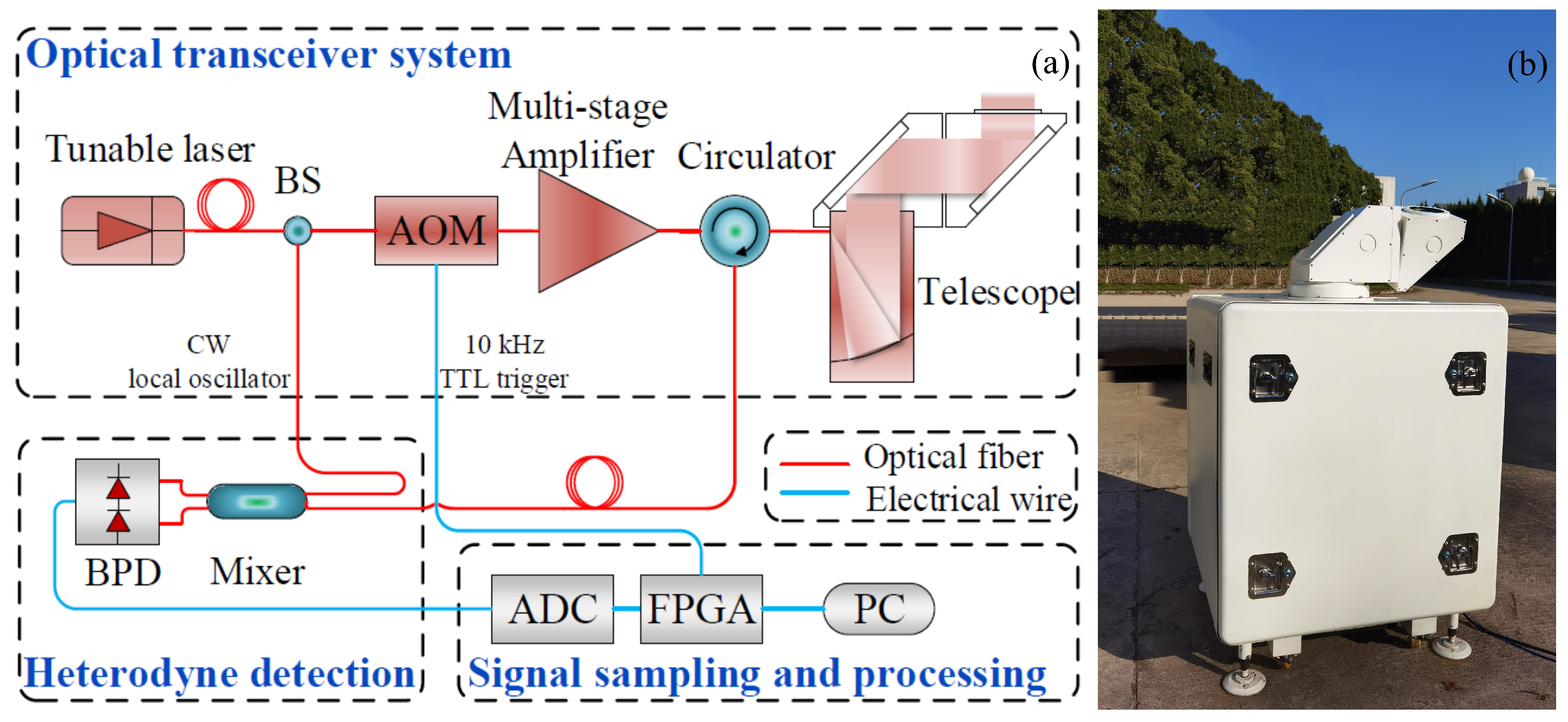
Coherent wind lidar is based on optical heterodyne detection technology and the Doppler effect principle for atmospheric wind field detection. The Windviewer100s system constructed in this study is illustrated in Figure 1. A continuous wave (CW) laser source produced by a tunable laser (center wavelength 1550 nm and linewidth 5 kHz) is modulated by an acousto-optic-modulator (AOM), and it is amplified by a multi-stage erbium-doped fiber amplifier (EDFA) to generate an optical pulse with an 80 MHz frequency shift, 10 kHz repetition rate, and 110 J pulse energy. The pulse is then propagated through an optical circular, and then output through an off-axis parabolic telescope to achieve laser beam expansion, which is sent to the atmosphere for interaction with atmospheric aerosols. The backscattered light signals from the interaction return along the laser line of sight, and they are collected by the same telescope, which is then output through the other port of the optical circulator. It is coupled into a 2 × 2 polarization that maintains a fiber coupler mixed with the continuous local oscillator light for heterodyne mixing. The mixed optical signal is then converted into an electrical signal by a balanced photodetector (BPD), which is collected into digital signals by an ADC and processed by a FPGA. To achieve various scanning modes such as Doppler beam swinging (DBS), velocity azimuth display (VAD), plan position indicator (PPI), and range height indicator (RHI) [32], two flat mirrors with two degrees of rotation freedom are installed in the scanning device, and the expanded laser beam is directed to the desired direction via the drive mechanism. The trigger signal for the AOM is generated in real-time at a 10 kHz frequency by the FPGA. Detailed technical specifications for the system are listed in Table 1. Assuming that the total efficiency is 0.5, we can compute that figure of merit (FOM) for Windviewer100s is 15, and that the corresponding typical measurement range is about 4 km [28].
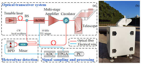
Figure 1.
The schematic structure and a photograph of the Windviewer100s lidar system. (a) Schematic diagram of the system, which contains the following three main parts: an optical transceiver system, a heterodyne detection system, and a signal sampling and processing system. BS: beam splitter; CW: continuous-wave laser; AOM: acousto-optic modulator; TTL: transistor–transistor logic; BPD: balanced photodetector; ADC: analog-to-digital converter; FPGA: field-programmable gate array; and PC: personal computer. (b) Photograph of the system in operation. The volume is about 820 mm (Length) × 820 mm (Width) × 1350 mm (Height).

Table 1.
Main technical specifications of the Windviewer100s.
The frequency of the backscattered light signal received through the telescope contained both the frequency of the transmitted light signal and the frequencies caused by the motion of aerosols. When combining the heterodyne detection technology and the Doppler effect principle, the relationship between the wind speed component along the laser line of sight and the Doppler frequency shift caused by the motion of aerosols is as follows:
where is the wind speed component along the laser line of sight, is the Doppler frequency shift, and is the wavelength of the transmitted light beam.
Coherent Doppler wind lidar synthesizes atmospheric wind fields by measuring the radial wind speed in different directions. Common modes include the VAD mode and DBS mode. The VAD mode continuously scans the radial velocity at different azimuths with a fixed elevation angle, and one cycle of a multi-beam measurement is equivalent to multiple cycles of the DBS mode, which is suitable for observing unstable atmospheric environments. The DBS mode has fewer scanning beams, shorter measurement cycles, and can improve data update rates. Depending on the value of the radial wind speed used in measurement and inversion, the DBS mode can be divided into the three-beam method (DBS3), four-beam method (DBS4), and five-beam method (DBS5). Windviewer100s uses the four-beam method, in which the radial wind speed is measured sequentially in the north, east, south, and west directions in a loop. The synthesis of the horizontal wind speed and wind direction is as follows:
where is the zenith angle, is the radial wind speed in the east, is the radial wind speed in the west, is the radial wind speed in the north, is the radial wind speed in the south, u is the east-west velocity component, v is the north–south velocity component, and w is the vertical velocity component. Thus, the horizontal wind speed and wind direction can be expressed as follows:
where is the horizontal wind speed and is the wind direction. The scanner maintains a uniform rotation speed of 15/s, and its initiation and termination involve acceleration and deceleration processes, thus introducing a delay when transitioning from 0 to 15/s and vice versa. Consequently, the update time for radial wind speed is approximately 10 s. During continuous scanning measurements, the interval between successive reconstructions of the horizontal wind speed and wind direction should match the update time of the radial wind speed. The entire four-beam scan cycle takes approximately 40 s.
2.2. Key Preprocessing Algorithm
The wind speed measurement range of coherent wind lidar determines the frequency range of the intermediate frequency (IF) signal in the photodetector. For example, if the wind speed measurement range is ±30 m/s, the highest IF signal frequency, as calculated using Equation (1), is 118.7 MHz (including the 80 MHz frequency shift generated by the AOM). According to the Nyquist sampling theorem, the sampling frequency of the data acquisition card must be at least greater than 237.4 MHz.
This paper realizes the synchronous acquisition and computation of echo signals in coherent wind lidar based on FPGA. The specific hardware block diagram is shown in Figure 2. The signal acquisition and processing module is equipped with a Xilinx KINTEX-7 on-chip FPGA chip (Model: FPGA-XC7K325T-2FFG900i, Xilinx Inc., San Jose, CA, USA). When taking the high-performance FPGA as the main control unit, an ADC chip (Model: AD9680, Analog Devices, Inc., Norwood, MA, USA) with a 14-bit resolution and clock management circuit was used to control and process the acquired data. In order to transfer the pre-processed data to the host computer, we used some high-speed communication interfaces such as Ethernet or USB3.0. In addition, a single-channel 4 GB/64 bit DDR3 (Double Data Rate, Micron Technology Inc., Boise, ID, USA) chip set external to the FPGA was also included, thereby achieving a peak rate of greater than 4400 MB/s. The FPGA was equipped with a 256 MB SPI Flash for program storage and booting, with LED indicators showing the loading and normal operation status. The ADC acquisition circuit provided two input channels, where the Ain0 channel realized a low-to-medium frequency acquisition of 2 GHz without gain, and the Ain1 channel realizes the acquisition of signals with a maximum gain of 35 dB and a frequency range of up to 600 MHz. A single external trigger signal with 10 kHz frequency provides a laser pulse trigger signal to the fiber laser, thereby sharing a common reference clock with the option of synchronized acquisition, which stabilizes the coherent wind lidar echo signal acquisition. We can use the PLL (phase-locked loop) of the external reference clock for the FPGA. The overall dimensions after assembly were 143 mm × 107 mm × 46.8 mm, which means that the build is characterized by small size, ease of interaction, strong real-time performance, and high integration.
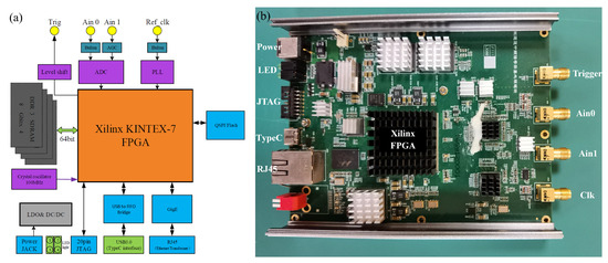
Figure 2.
Schematic of the hardware composition and a photograph of the signal acquisition and processing module. (a) Hardware schematic diagram, which mainly contains ADC circuits, a Xilinx KINTEX-7 on FPGA chip, DDR3 memory, and external interfaces. (b) Photograph of the minimal implementation setup and the carrier board with a FPGA-XC7K325T-2FFG900i mounted. In the left part of the image there is the power supply and network communication interface; in the right part, the external trigger signal provides a laser pulse trigger signal to the fiber laser Ain 0 or Ain 1 channel for collecting IF signals.
Due to the influence of factors such as the detection target, detection aperture, and emission power, the power of the backscatter echo signal detected by the lidar was at the nW level with an extremely low carrier-to-noise ratio (CNR). Additionally, external environmental factors such as atmospheric extinction, atmospheric turbulence, atmospheric scattering, as well as internal factors such as shot noise and thermal noise in the photoelectric detection unit, also reduce the CNR of the echo signal. Therefore, the echo signal is divided into multiple range gates. Initially, the FFT and power spectrum of each range gate were calculated for a single emitted pulse. Subsequently, the power spectra of multiple emitted pulses were non-coherently accumulated, and, finally, the peak of the Doppler frequency was retrieved from the accumulated power spectra [24]. Using the frequency domain non-coherent accumulation estimation method can improve the wind speed estimation accuracy of coherent wind lidar without affecting the range resolution. However, accumulating power spectra from multiple emitted laser pulses can reduce the temporal resolution of wind speed measurements and increase the data volume of signal acquisition and processing.
For the data processing of the coherent wind lidar with a time resolution of 1 s, a spatial resolution of 30 m, a long-range detection up to 9.9 km, and a pulse repetition rate of 10 kHz, a straightforward approach would be to instantiate 329 FFT IP cores (each with a length of 512 points). The time domain echo signals were buffered and then sent to each FFT IP core for processing. With a clock frequency of 100 MHz, performing a 512-point real FFT took approximately 16.4 s. When the high-speed ADC sampling rate was 400 MS/s, collecting echo signals within a 9.9 km range and calculating the FFT for the last group of range gates took a total time of 82 s (within a 100 s laser pulse time). Though this data processing method is simple and easy to maintain in software, it consumes a substantial amount of FPGA hardware resources.
This paper proposes the employment of multi-phase decomposition technology and a pipelining approach to distribute the 329 range gates evenly to 7-channel multi-phase FFT calculation modules. Each channel employs an N-point multi-phase FFT with a base-4 configuration, in which the serial FFT algorithm is converted into a parallel multiphase FFT algorithm with multiple independent signal branches that can simultaneously perform FFT calculations [33]. Figure 3 illustrates the specific workflow of real-time signal acquisition and accumulation power spectrum calculation based on FPGA. The high-speed ADC performs a real-time acquisition of time domain echo signals for each emitted laser pulse. A programmable sliding window divides the collected signal sequence into range gates, and assigns them alternately in the order of the range gates to the 7-channel multi-phase FFT calculation modules. Each multi-phase FFT calculation module is assigned 47 range gate data and carries out the same spectral calculation process. It completes the fast Fourier transform and power spectrum calculation for all pre-set range gates within one emitted laser pulse period while simultaneously caching the calculation results of the corresponding range gates to the accumulation register. Upon the arrival of the next emitted laser pulse, the accumulation register for the same range gate completes accumulation. When the number of spectrum accumulations reaches the pre-designed 10,000 emitted laser pulses, one measurement cycle is completed. Each channel’s FFT calculation module reorders and transfers the real-time pre-processed power spectrum accumulation results via Gigabit Ethernet to the host computer. Further wind speed information extraction is carried out through a spectral estimation algorithm post-processing module. After completing one measurement cycle, the FPGA clears the accumulation register and the pulse count accumulation, thus starting the calculation for the next measurement cycle, as well as ensuring continuous data acquisition and processing. The coherent wind lidar estimates the Doppler frequency based on spectral distribution, and the algorithms include the periodogram maximum likelihood estimation algorithm, Gaussian fitting estimation algorithm, parabolic fitting estimation algorithm, centroid spectral estimation algorithm, etc. [24,34,35]. Among them, the periodogram maximum likelihood estimation algorithm is simple in form, has a small computational load, and its accuracy depends on the frequency resolution; the Gaussian fitting estimation algorithm optimizes the periodogram maximum likelihood estimation to improve frequency estimation accuracy, and its computational load is moderate; the centroid spectral estimation algorithm has a smaller computational load compared to the Gaussian fitting estimation algorithm, and it is more suitable for measurement environments where irregular Doppler peaks may appear. Considering the real-time measurement and environmental adaptability of coherent wind lidar, this paper adopts the centroid spectral estimation algorithm.
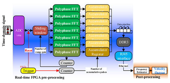
Figure 3.
Real-time acquisition and processing algorithm based on FPGA.
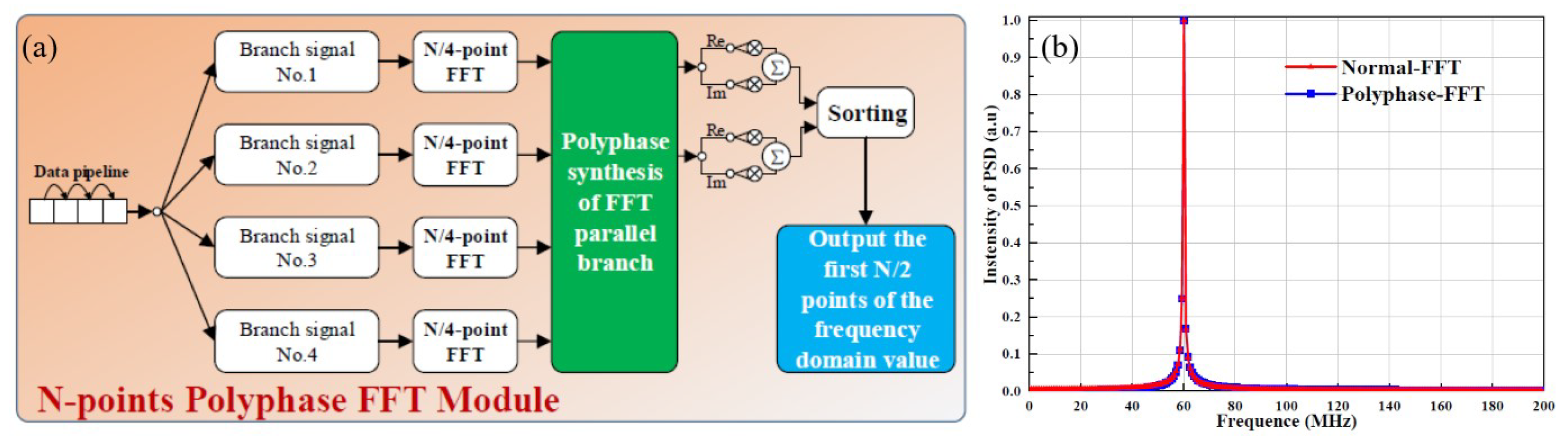
When the ADC sampling rate is 400 MS/s, the FPGA corresponds exactly to four sampling points at a clock frequency of 100 MHz. Each channel’s FFT module employs a radix 4 N-point multi-path FFT, where four branches simultaneously perform N/4-point FFT calculations. After each branch completes a serial FFT of N/4 points and multiplies it by a rotation factor, a two-dimensional parallel FFT calculation is performed. The results are then adjusted and sorted to obtain the signal frequency domain values with N points, as illustrated in the algorithm’s principle in Figure 4a. The time-domain digital signals collected by the ADC are represented as . The time domain expressions of the baseband signals for the four branches are given as follows:
where n is the sample index (0 to ) and r represents the branch index (0 to 3). The FFT results of the time domain for each branch can be represented as follows:
where k represents the FFT point index for each branch. The corresponding rotation factors for each branch are as follows:
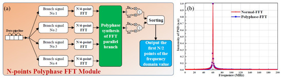
Figure 4.
Schematic diagram of multi-path FFT calculation. (a) Principle flowchart. (b) Multi-path FFT simulation.
In practical applications, the time domain signal data acquired by the ADC are real, and the FFT of the real data exhibits a conjugate symmetric property in the frequency domain. Only half of the frequency domain information was valid, thus resulting in some redundant computations in the frequency domain transformation. Therefore, in the multi-path FFT algorithm structure, only the magnitude square sum of the first N/2 frequency domain points was computed. Using the VIVADO [36] tool integrated design environment, the calculation results of a 512-point multi-path FFT for simulated data with a signal frequency of 60 MHz and a sampling rate of 400 MS/s are shown in Figure 4b. The calculated peak frequency was 60.16 MHz, and this is consistent with the results of serial FFT calculations, thus verifying the feasibility of this algorithm.
The signal acquisition and processing algorithm using multi-path decomposition and a pipeline structure do not require storing the time domain data acquired by the ADC; moreover, they can directly achieve the fast pipelined processing of data, thus saving hardware resource utilization. The radix-4 multi-path FFT reduces the number of computation points for a single FFT, thereby reducing the data processing time to 1/4 of the time required for serial FFT calculations, and thus improving the data transmission and processing efficiency. Through actual calculations, the time required to complete FFT processing within a single laser pulse for a detection range of 9.9 km did not exceed 72 s, thus meeting the requirement for processing within 100 s.
3. Experiment and Results
3.1. Detection Measurement
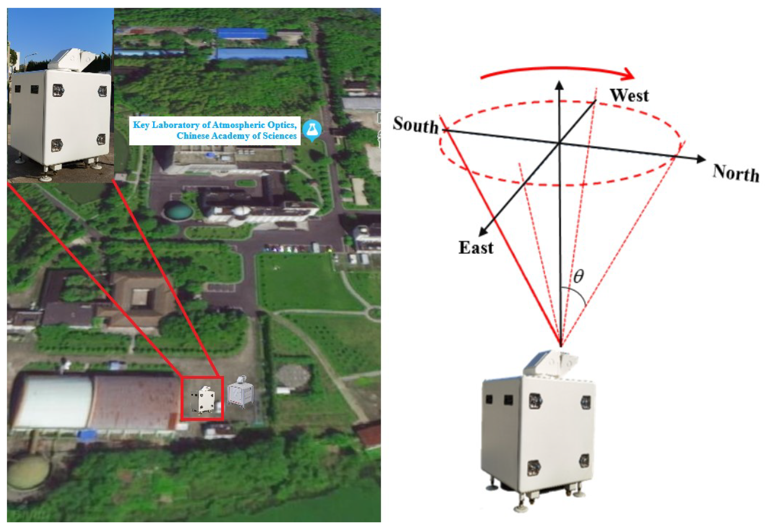
After the system was assembled, measurements were conducted in September 2022 at the Key Laboratory of Atmospheric Optics, Chinese Academy of Sciences (31545N, 117107E), as shown in Figure 5. The Windviewer100s coherent wind lidar developed in this study and the Windcube100s scanning lidar produced by Leosphere, in France, were simultaneously used for measurements. The two lidars were positioned 10 m apart, and the measurements were conducted using a Doppler beam scanning mode with a zenith angle of 15. The main performance parameters of the Windcube100s are shown in Table 2, and it can measure the horizontal wind speed and wind direction in the vertical range of 50 m to 3170 m. The threshold of the CNR for the Windcube100s to reconstruct horizontal wind speed and wind direction was −26.5 dB.
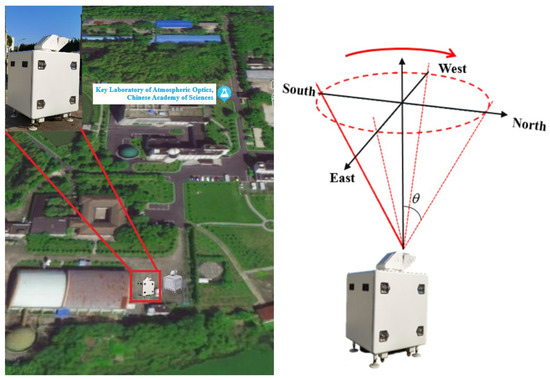
Figure 5.
The installation position and measurement method of the coherent wind lidar.
Table 2.
Main technical parameters of Windcube100s [12].
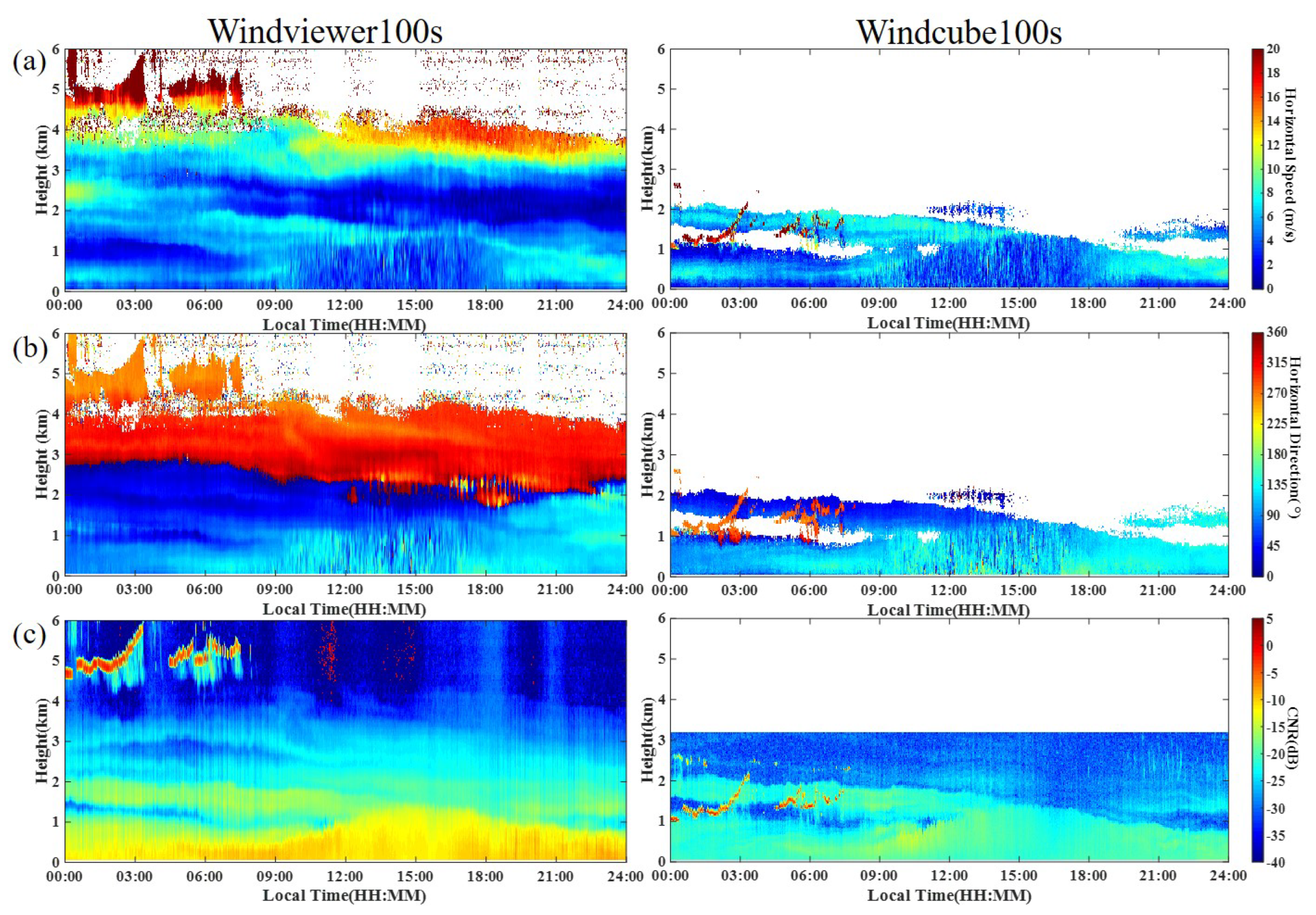
Figure 6 presents the horizontal wind speed and wind direction results measured continuously for one day on 5 November 2022. Some of the data were discarded by Windviewer100s when their CNR was lower than −36.5 dB. The stable measurement height of the Windviewer100s reached up to 4000 m above the atmospheric boundary layer. The atmospheric boundary layer is the transitional region between the lower atmosphere and the turbulent transport near the Earth’s surface. The concentration of aerosols below the atmospheric boundary layer was significantly higher than in the free atmosphere above the boundary layer. When the aerosol concentration was high, the backscattered light signal received by the coherent wind lidar became stronger. The CNR distribution of the corresponding measurement data showed that, on the measurement day, the height of the atmospheric boundary layer increased to 1500 m around 3:00 p.m. Above 1500 m, the CNR weakened, and the variation was relatively stable. Due to the lower pulse repetition rate of Windviewer100s (10 kHz) compared to Windcube100s (40 kHz), there was no ambiguity in the Windviewer100s measurements below 3 km. The developed coherent wind lidar processed the acquired time domain signals directly through FPGA to obtain spectral data. When combined with the centroid spectral estimation algorithm, it could retrieve wind field data, even under low CNR conditions, thus improving the overall measurement capability.
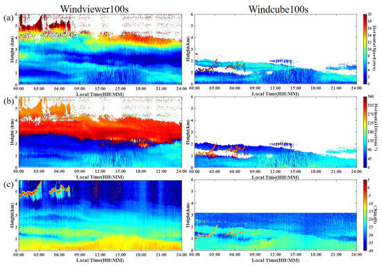
Figure 6.
Windviewer100s and Windcube100s measurement results. (a) Horizontal wind speed, (b) wind direction, and (c) CNR.
3.2. Detection Altitude
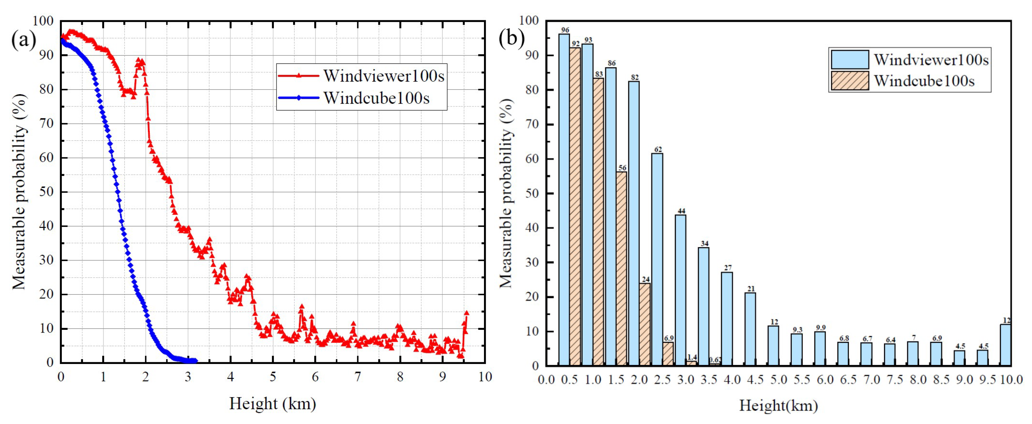
Between 29 September 2022, and 2 December 2022, both coherent wind lidars operated continuously and normally, thereby providing all-weather observations of the atmospheric wind field above. During this period, the effective detection time was about 887 h (days with multiple occurrences of rainy weather were not included in the effective detection time statistics). Figure 7 shows the data acquisition rate of the effective measurements at different detection altitudes during the measurement period, with altitude intervals of 500 m. It can be observed that, as the altitude increases, the effective data acquisition rate gradually decreases. The measurement range of the Windviewer100s extends from 58 m to 9567 m. Within the same measurement time frame, the effective data acquisition rate of the Windviewer100s was higher than that of the Windcube100s, and it can measure higher altitudes. In the altitude range of 0–500 m, 500–1000 m, and 1000–1500 m, both lidars achieved an effective data acquisition rate of over 50%. The data acquisition rate of the Windcube100s decreased to 24% at altitudes of 1500–2000 m, and was only 6.9% at altitudes of 2000–2500 m, while the corresponding rates for the Windviewer100s reached 82% and 61%, respectively. The aerosol boundary layer height in the Hefei area typically varies between 500–1500 m, and the developed coherent wind lidar has the capability to detect high-altitude atmospheric wind fields above the boundary layer.
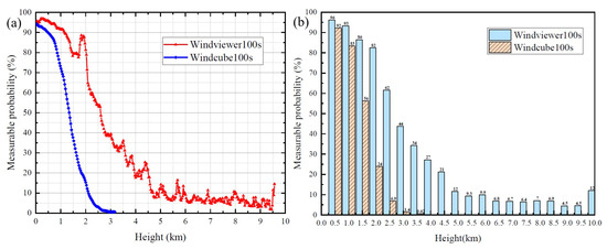
Figure 7.
Effective data acquisition rate of the coherent wind lidar. (a) Statistics by detection altitude and (b) statistics with 500 m height intervals.
3.3. Comparison Experiments of Lidars and Radiosonde
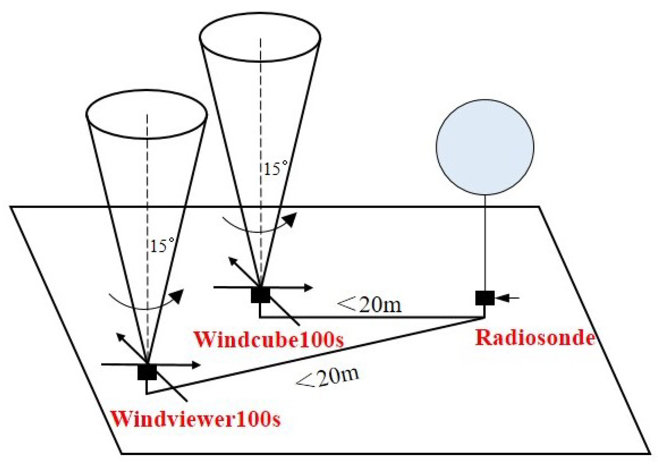
Radiosonde is a standard method for atmospheric wind field measurements that uses ground antennas to receive response signals from instruments carried by weather balloons. It is widely used in meteorological observations to validate the accuracy of coherent wind lidar measurement data. In this study, a radiosonde was used, and Table 3 provides the main performance parameters of the radiosonde. Figure 8 illustrates the comparison test, with the release point of the weather balloon located less than 20 m from the coherent wind lidar observation point.
Table 3.
Main technical parameters of radiosonde.

Figure 8.
Position of the equipment during the three measurement experiments.
Due to the different principles of the coherent wind lidar and radiosonde for measuring atmospheric wind fields, there were differences in their measurement time resolution and spatial resolution. In actual measurements, the coherent wind lidar observed wind profiles above vertically, while the weather balloon ascended at an average speed of about 4 m/s and collected wind profile data along its path. In order to avoid the influence of range ambiguity, we chose clear and cloudless weather to carry out the comparison experiments of the lidars and radiosonde. The Windviewer100s coherent wind lidar has a data update rate of approximately 10 s and a height resolution of 29 m, while the Windcube100s has a data update rate of about 5 s and a height resolution of 30 m. The radiosonde measures wind speed and wind direction with a data update rate of 1 s and a height resolution of about 4 m. Through considering the vertical spatial resolution of all three systems, the wind speed and wind direction data were matched for adjacent heights with a height difference of no more than 3 m in the observed data. Additionally, the coherent wind lidar’s observation data were vector-averaged at the minute level to reduce the impact of instantaneous winds. For a vertical measurement height of 3.5 km with the coherent wind lidar, and when considering the vertical ascent speed of the radiosonde, it takes approximately 14.5 min to reach a height of 3.5 km. Therefore, the coherent wind lidar observation data were averaged over 15 min, and they corresponded to the observed atmospheric wind field data at the height where the radiosonde operates.
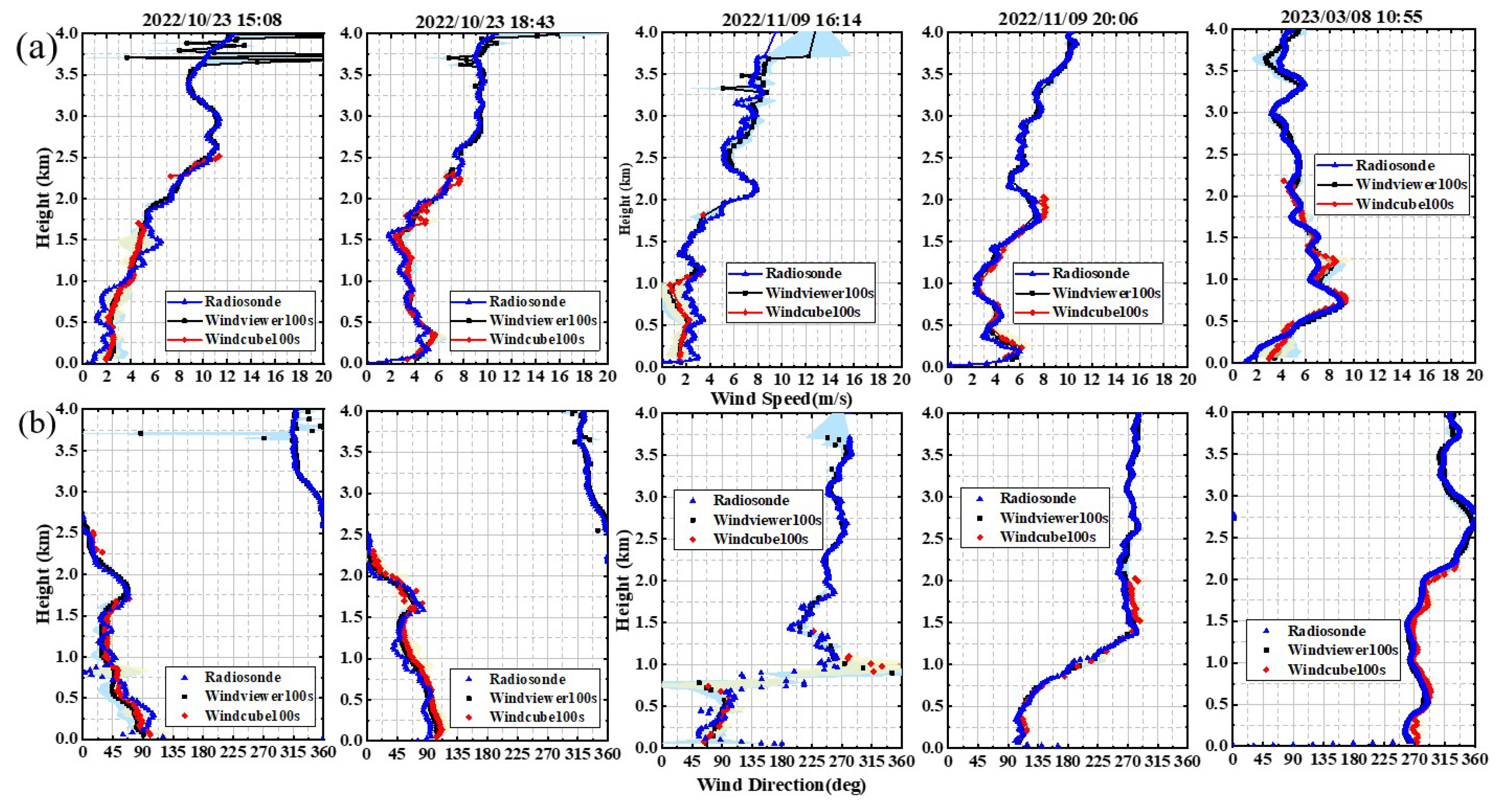
To ensure continuous and normal observations by the coherent wind lidar during radiosonde operations, the release time of the weather balloon was recorded. During the observation and comparison period, five weather balloons were released, and they corresponded to the local times of 15:08 on 23 October 2022, 18:43 on 23 October 2022, 16:14 on 9 November 2022, 20:06 on 9 November 2022, and 10:55 on 8 March 2022. Figure 9 presents the results of the observation data comparison.
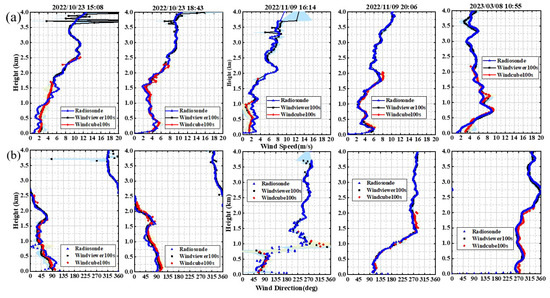
Figure 9.
Comparison of the coherent wind lidar and radiosonde observation results. (a) Horizontal wind speed and (b) wind direction.
The atmospheric wind field data (including horizontal wind speed and wind direction) obtained by the radiosonde and the coherent wind lidar at the different detection altitudes of the matched samples were within a height difference of 3 m. The deviations in the observed data from both instruments were calculated to obtain the mean error (ME) and root mean square error (RMSE) values of the wind speed and wind direction, which were measured by the coherent wind lidar at various altitudes. To avoid calculating false wind direction deviations due to the 0 to 360 range of wind direction, the wind direction differences were computed as the angles between vectors (e.g., when the wind direction measurement values were 355 and 5, the difference should be 10) to ensure reasonable wind direction deviation values. The results presented in Table 4 show that, in the late afternoon, the RMSE values of the horizontal wind speed measured by the Windviewer100s coherent wind lidar and the radiosonde were 0.434 m/s and 0.332 m/s, respectively, with wind direction deviation values of 7.204 and 5.522, respectively. When compared to the radiosonde, the Windcube100s coherent wind lidar had RMSE values of the horizontal wind speed of 0.548 m/s and 0.611 m/s, and wind direction deviation values of 12.965 and 9.795, respectively, which are significantly smaller than the deviations observed during the afternoon measurements. Due to the increased turbulence caused by surface heating, low-level effects were generally more pronounced below 1000 m in altitude, which resulted in significantly larger deviations below 1000 m in the results from 23 October 2022 at 15:08 and 9 November 2022 at 16:14, as shown in Figure 9.
Table 4.
Comparison results between the Windviewer100s (A lidar) and Windcube100s (B lidar).
Figure 10 statistically analyzes the correlation of five comparative measurements, in which the wind direction is selected in the range of 7.5 to 352.5 to avoid the statistical illusion caused by approaching the true north angle (0). Coherent wind lidar is highly correlated with the observed values of horizontal wind speed and the wind direction of sounding balloons at different heights. The correlation coefficients of Windviewer100s horizontal wind speed and wind direction were 0.992 and 0.999, respectively. The average deviation of wind speed was −0.15 m/s, the root mean square error was 0.56 m/s, the average deviation of wind direction was −0.23, and the root mean square error was 8.40. The correlation coefficients of Windcube100s horizontal wind speed and wind direction were 0.983 and 0.997, respectively, and the average deviation of wind speed was −0.20 m/s, the root mean square error was 0.69 m/s, the average deviation of wind direction was −5.98, and the root mean square error was 11.08. Since the wind direction spans from 0–360, in order to avoid inaccuracies in the assessment of the wind direction, the wind direction and wind speed were converted into u and v wind fields, respectively. Figure 10c,d statistically analyze the correlation of u and v. They are highly correlated with the observed values of the u and v of the radiosonde at different heights. The correlation coefficients of Windviewer100s u and v were 0.984 and 0.986, respectively. The average deviation of u was −0.01 m/s, the root mean square error was 0.59 m/s, the average deviation of v was 0.03 m/s, and the root mean square error was 0.51 m/s. The correlation coefficients of Windcube100s’ u and v were 0.973 and 0.908, respectively, and the average deviation of u was 0.12 m/s, the root mean square error was 0.74 m/s, the average deviation of v was 0.15 m/s, and the root mean square error was 0.83 m/s. The above results showed that the u and v measurement deviation of Windviewer100s was than that of Windcube100s. The above results showed that the integrated scheme of signal acquisition and processing based on FPGA proposed in this paper can be applied to the coherent wind lidar system, and it can also achieve the detection accuracy of the Windcube100s.
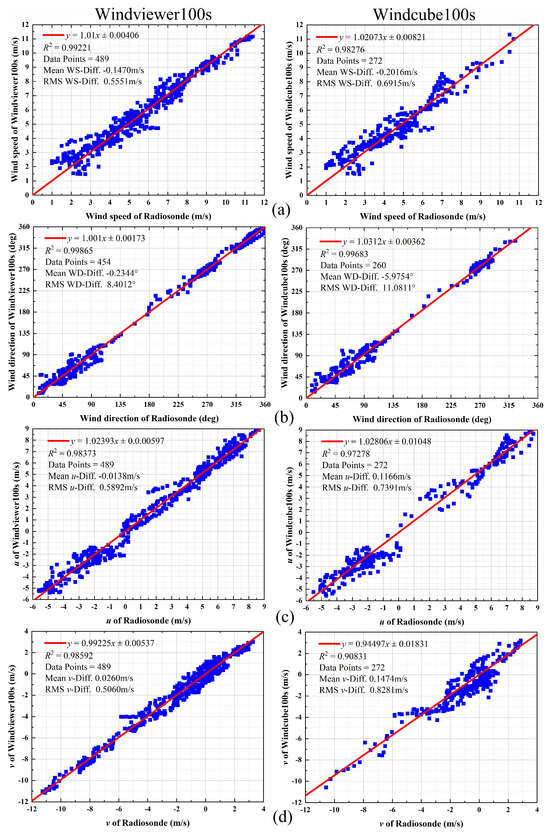
Figure 10.
Linear analysis of Windviewer100s and Windcube100s. (a) Wind speed, (b) wind direction, (c) the u component of wind speed, and (d) the v component of wind speed.
4. Discussion
The continuous 24 h measurement results confirmed that the FPGA-based real-time signal acquisition and processing integrated module can be applied to coherent Doppler wind lidar. The module is small in size, low in power consumption, and has an external trigger function, thus ensuring synchronization between the echo signal acquisition and laser pulse. The use of a multi-channel multi-phase FFT algorithm can achieve the real-time preprocessing of the spectral data of 329 distance gates in coherent Doppler wind lidar, thus reducing the data volume uploaded to the host computer. This approach can be directly applied to smaller coherent Doppler wind lidar in the future.
During the continuous 24 h measurement period from 09:00 to 16:30, the atmospheric wind direction changed rapidly; this was especially the case when below 1000 m, where intense near-surface convection occurs and generates strong turbulence. For atmospheric turbulence and fluctuations, the atmospheric wind field displayed disturbances and fluctuations in wind speed and direction. After 16:30, due to the lower solar elevation angle, the warming effect on the ground weakened, thereby making the entire atmosphere more stable. For a data cycle of 10 s in atmospheric wind field measurement, coherent Doppler wind lidar can be used for the continuous observation of atmospheric dynamics processes. Windviewer100s has a higher CNR below the boundary layer compared to Windcube100s under the same atmospheric conditions. The CNR drops below −30 dB when it exceeds 2 km, thus making it impossible for Windcube100s to extract wind speed information. In contrast, Windviewer100s continues to operate, even at higher altitudes such as 4 km. In low CNR conditions, wind speed information can be extracted from the spectral information of the multi-channel multi-phase FFT algorithm. Moreover, the CNR of coherent Doppler wind lidar is influenced by both the atmospheric environment and system parameters, thereby resulting in differences in the CNR threshold between different measurement devices.
The comparison experimental results showed that the measurement results of Windviewer100s, Windcube100s, and the horizontal wind speed and wind direction measured by radiosonde have good consistency. Also, during 09:00 to 16:30, the deviation between coherent Doppler wind lidar and radiosonde was significantly larger than in the evening, and this corresponded to the influence of atmospheric turbulence and fluctuations on the measurement results during noon. In terms of evaluating measurement accuracy, besides the influence of the calculation method itself, it is also affected by the radiosonde equipment. Lidar uses the Doppler frequency of backscattered light to determine wind speed, with the errors mainly coming from the CNR of the echo signal and the resolution of the data acquisition. Radiosonde measures the change in spatial position at fixed time points to calculate wind speed. Although the lidar and radiosonde release points are very close, the radiosonde may experience undirected horizontal drift during ascent and thus deviate from the initial release position. Therefore, larger spatial displacement may affect the consistency of the lidar and radiosonde observation results. According to the measurement accuracy of the radiosonde horizontal wind speed and wind direction, as well as the comparative results detailed in Section 3.3, the wind speed values below a 3.5 km height during the measurement period were small, and the measurement deviation caused by the radiosonde spatial displacement can be ignored.
5. Conclusions
An all-fiber coherent Doppler wind lidar (Windviewer100s) was developed for long-range real-time wind reconstruction based on an FPGA real-time acquisition and processing integrated solution. The FPGA processing system was used to convert the analog echo signal of the coherent wind lidar into a digital signal in real time, thus enabling synchronous acquisition and calculation. The multi-phase decomposition technique and pipeline structure were used to distribute an aerosol particle echo signal data to seven sets of FFT modules. After the FPGA completed the real-time acquisition of the echo signal and complex spectral calculation preprocessing, it was transmitted to the host computer for post-processing with the spectral centroid estimation algorithm to extract velocity, thereby addressing the issue of large data volume and computation in the wind speed inversion of the coherent wind lidar.
Through measurement experiments, it was demonstrated that the coherent Doppler wind lidar system using the real-time acquisition and processing integrated solution could extract wind speed information from low CNR data, thus enabling a continuous 24 h measurement wind field with the effective detection altitudes exceeding the atmospheric boundary layer. Simultaneous and co-located observations were conducted using a radiosonde and Windcube100s lidar. The effective data rate of the Windviewer100s lidar at different detection altitudes during the measurement period was statistically analyzed. The results showed that, in the altitude range of 1500–2000 m and 2000–2500 m, the effective data rates of Windviewer100s were 82% and 61%, respectively. Moreover, the Windviewer100s lidar had a detection altitude of over 4.0 km, as well as a wind speed and direction measurement deviation better than 0.6 m/s and 9 within the 3.5 km range, respectively (with correlations exceeding 0.99).
In conclusion, the feasibility of the FPGA-based real-time acquisition and processing integrated solution has been confirmed. This module severs as an important research foundation for the development of compact and robust coherent Doppler wind lidar systems—ones that are suitable for various scientific applications.
Author Contributions
Conceptualization, Q.L. and X.J.; methodology, Q.L. and X.J.; validation, W.Z. and C.Q.; data analysis, Q.L. and X.J.; writing-original draft preparation, Q.L.; writing-review and editing, Q.L., X.J. and C.Q. All authors have read and agreed to the published version of the manuscript.
Funding
This work was supported by the Director Fund of State Key Laboratory of Pulsed Power Laser Technology (grant no. SKL2021ZR09), the Research Fund of State Key Laboratory of Pulsed Power Laser Technology, and the Foundation of Advanced Laser Technology Laboratory of Anhui Province (grant no. AHL2021QN02).
Data Availability Statement
The data underlying the results presented in this study are not publicly available at this time but may be obtained from the authors upon reasonable requirement.
Conflicts of Interest
The authors declare no conflict of interest.
References
- Stanley, G.B.; Barry, E.S.; Eduard, J.S.; Koch, S.E. The value of wind profiler data in U.S. weather forecasting. Bull. Am. Meteorol. Soc. 2004, 85, 1871–1886. [Google Scholar]
- Banakh, V.A.; Werner, C. Computer simulation of coherent Doppler lidar measurement of wind velocity and retrieval of turbulent wind statistics. Opt. Eng. 2005, 44, 071205. [Google Scholar]
- Cezard, N.; Mehaute, S.L.; Gout, J.L.; Valla, M.; Goular, D.; Fleury, D.; Planchat, C.; Dolfi-Bouteyre, A. Performance assessment of a coherent DIAL-Doppler fiber lidar at 1645 nm for remote sensing of methane and wind. Opt. Express 2020, 28, 22345–22357. [Google Scholar] [CrossRef] [PubMed]
- Wu, S.H.; Zhai, X.C.; Liu, B.Y. Aircraft wake vortex and turbulence measurement under near-ground effect using coherent Doppler lidar. Opt. Express 2019, 27, 1142–1163. [Google Scholar] [CrossRef] [PubMed]
- Reitebuch, O. Wind Lidar for Atmospheric Research. In Atmospheric Physics; Schumann, U., Ed.; Springer: Berlin/Heidelberg, Germany, 2012; pp. 487–507. [Google Scholar]
- Kliebisch, O.; Uittenbosch, H.; Thurn, J.; Mahnke, P. Coherent Doppler wind lidar with real-time wind processing and low signal-to-noise ratio reconstruction based on a convolutional neural network. Opt. Express 2022, 30, 5540–5552. [Google Scholar] [CrossRef] [PubMed]
- Zhao, Y.; Yuan, L.C.; Fan, C.H.; Zhu, X.P.; Liu, J.Q.; Dai, B.; Xiao, W.G.; Zhu, X.L.; Chen, W.B. Wind retrieval for genetic algorithm-based coherent Doppler wind lidar employing airborne platform. Appl. Phys. B Lasers Opt. 2023, 129, 36–46. [Google Scholar] [CrossRef]
- Vasiljević, N.; Lea, G.; Courtney, M.; Cariou, J.P.; Mann, J.; Mikkelsen, T. Long-range windscanner system. Remote Sens. 2016, 8, 896. [Google Scholar] [CrossRef]
- Fujii, T.; Fukuchi, T. Laser Remote Sensing; CRC Press: Boca Raton, FL, USA, 2005. [Google Scholar]
- Huffaker, R.M. Laser Doppler detection systems for gas velocity measurement. Appl. Opt. 1970, 9, 1026–1039. [Google Scholar] [CrossRef]
- Banakh, V.A.; Smalikho, I.N. The impact of internal gravity waves on the spectra of turbulent fluctuations of vertical wind velocity in the stable atmospheric boundary layer. Remote Sens. 2023, 15, 2894. [Google Scholar] [CrossRef]
- Cariou, J.; Sauvage, L.; Thobois, L.; Gorju, G.; Machta, M.; Lea, G.; Duboué, M. Long range scanning pulsed Coherent Lidar for real time wind monitoring in the Planetary Boundary Layer. In Proceedings of the 16th Coherent Laser Radar Conference 2011 (CLRC XVI), Long Beach, CA, USA, 20–24 June 2011. [Google Scholar]
- Diao, W.F.; Zhang, X.; Liu, J.Q.; Zhu, X.P.; Liu, Y.; Bi, D.C.; Chen, W.B. All fiber pulsed coherent lidar development for wind profiles measurements in boundary layers. Chin. Opt. Lett. 2014, 12, 072801. [Google Scholar] [CrossRef]
- Wang, C.; Xia, H.Y.; Shangguan, M.J.; Wu, Y.B.; Wang, L.; Zhao, L.J.; Qiu, J.W.; Zhang, R.J. 1.5 μm polarization coherent lidar incorporating time-division multiplexing. Opt. Express 2017, 25, 20663–20674. [Google Scholar] [CrossRef]
- Liu, H.; Zhu, X.F.; Fan, C.H.; Bi, D.C.; Liu, J.Q.; Zhang, X.; Zhu, X.L.; Chen, W.B. Field performance of all-fiber pulsed coherent Doppler lidar. In Proceedings of the 29th International Laser Radar Conference, Heifei, China, 24–28 June 2019. [Google Scholar]
- Abdelazim, S.; Santoro, D.; Arend, M.; Moshary, F.; Ahmed, S. Signal to Noise Ratio Characterization of Coherent Doppler Lidar Backscattered Signals. In Proceedings of the 27th International Laser Radar Conference, New York, NY, USA, 5–10 July 2015. [Google Scholar]
- Kameyama, S.; Ando, T.; Asaka, K.; Wadaka, S. Compact all-fiber pulsed coherent Doppler lidar system for wind sensing. Appl. Opt. 2007, 46, 1953–1962. [Google Scholar] [CrossRef]
- Saklakova, V.; Han, Y.L.; Zhang, S.H.; Qin, Z.; Xue, X.H.; Chen, T.D.; Sun, D.S.; Zhao, Y.M.; Zheng, J. Field programmable gate array-based coherent lidar employing the ordinal statistics method for fast Doppler frequency determinatio. Opt. Eng. 2022, 61, 124102. [Google Scholar] [CrossRef]
- Zhou, A.R.; Han, F.; Sun, D.S.; Han, Y.L.; Zheng, J.; Jiang, S. 1.55-μm pulse coherent LIDAR with 10-km detection range. Opt. Eng. 2019, 58, 096103. [Google Scholar] [CrossRef]
- Liang, C.; Wang, C.; Xue, X.H.; Dou, X.K.; Chen, T.D. Meter-scale and sub-second-resolution coherent Doppler wind LIDAR and hyperfine wind observation. Opt. Lett. 2022, 47, 3179–3182. [Google Scholar] [CrossRef]
- Rui, X.; Guo, P.; Chen, H.; Chen, S.Y.; Zhang, Y.C.; Zhao, M.; Wu, Y.W.; Zhao, P.T. Portable coherent Doppler light detection and ranging for boundary-layer wind sensing. Opt. Eng. 2019, 58, 034105. [Google Scholar] [CrossRef]
- Hardesty, R.M. Performance of a discrete spectral peak frequency estimator for Doppler wind velocity measurements. IEEE Trans. Geosci. Remote Sens. 1986, 24, 777–783. [Google Scholar] [CrossRef]
- Rye, B.J.; Hardesty, R.M. Discrete spectral peak estimation in incoherent backscatter heterodyne lidar. I. Spectral accumulation and the cramerrao lower bound. IEEE Trans. Geosci. Remote Sens. 1993, 31, 16–27. [Google Scholar] [CrossRef]
- Rye, B.J.; Hardesty, R.M. Discrete spectral peak estimation in incoherent backscatter heterodyne lidar. II. Correlogram accumulation. IEEE Trans. Geosci. Remote Sens. 1993, 31, 28–35. [Google Scholar] [CrossRef]
- Abdelazim, S.; Santoro, D.; Arend, M.; Moshary, F.; Ahmed, S. Field programmable gate array processing of eye-safe all-fiber coherent wind Doppler lidar return signals. In Proceedings of the SPIE Remote Sensing, Prague, Czech Republic, 19–22 September 2011; SPIE, The International Society for Optical Engineering: Bellingham, WA, USA, 2011. [Google Scholar]
- Abdelazim, S.; Santoro, D.; Arend, M.; Moshary, F.; Ahmed, S. A hardware implemented autocorrelation technique for estimating power spectral density for processing signals from a Doppler wind lidar system. Sensors 2018, 18, 4170. [Google Scholar] [CrossRef]
- Kliebisch, O.; Mahnke, P. Real-time laser Doppler anemometry for optical air data applications in low aerosol environments. Rev. Sci. Instrum. 2020, 91, 095106. [Google Scholar] [CrossRef]
- ISO 28902-2:2017; Air Quality–Environmental Meteorology–Part 2: Ground–Based Remote Sensing of Wind by Heterodyne Pulsed Doppler Lidar. ISO: Vernier, Switzerland, 2017.
- Kumer, V.-M.; Joachim, R.; Birgitte, R.; Furevik, A. Comparison of LiDAR and radiosonde wind measurements. Energy Procedia 2014, 53, 214–220. [Google Scholar] [CrossRef]
- Paschke, E.; Leinweber, R.; Lehmann, V. A one year comparison of 482 MHz radar wind profiler, RS92-SGP radiosonde and 1.5 μm Doppler lidar wind measurements. Atmos. Meas. Tech. Discuss. 2014, 7, 11439–11479. [Google Scholar]
- Bu, L.B.; Qiu, Z.J.; Gao, H.Y.; Zhu, X.P.; Liu, J.Q. All-fiber pulse coherent Doppler LIDAR and its validations. Opt. Eng. 2015, 54, 123103. [Google Scholar] [CrossRef]
- Rao, I.S.; Anandan, V.K.; Reddy, P.N. Evaluation of DBS wind measurement technique in different beam configurations for a VHF wind profiler. J. Atmos. Ocean. Technol. 2008, 25, 2304–2312. [Google Scholar] [CrossRef]
- Jung, Y.H.; Yoon, H.; Kim, J. New efficient FFT algorithm and pipeline implementation results for OFDM/DMT application. IEEE Trans. Consum. Electron. 2003, 49, 14–20. [Google Scholar] [CrossRef]
- Dolfi-Bouteyre, A.; Canat, G.; Lombard, L.; Matthieu, V.; Durécu, A.; Besson, C. Long-range wind monitoring in real time with optimized coherent lidar. Opt. Eng. 2019, 56, 031217. [Google Scholar] [CrossRef]
- Jiang, S.; Sun, D.S.; Han, Y.L.; Han, F.; Zhou, A.R.; Zheng, J. Performance of continuous wave coherent Doppler lidar for wind measurement. Curr. Opt. Photonics 2019, 3, 466–472. [Google Scholar]
- Feist, T. Vivado design suite. White Pap. 2012, 5, 30. [Google Scholar]


Disclaimer/Publisher’s Note: The statements, opinions and data contained in all publications are solely those of the individual author(s) and contributor(s) and not of MDPI and/or the editor(s). MDPI and/or the editor(s) disclaim responsibility for any injury to people or property resulting from any ideas, methods, instructions or products referred to in the content. |
© 2023 by the authors. Licensee MDPI, Basel, Switzerland. This article is an open access article distributed under the terms and conditions of the Creative Commons Attribution (CC BY) license (https://creativecommons.org/licenses/by/4.0/).