Abstract
Sporadic E (Es) layers are thin layers of enhanced electron density that commonly appear at altitudes of 90–130 km, often impacting radio communications and navigation systems. The wind shear theory posits that the vertical ion drift, influenced by atmospheric neutral winds and the magnetic field, serves as a significant dynamic driver for the formation and movement of Es layers. In current studies, both the heights of ion vertical velocity null (IVN) and the maximum vertical ion convergence (VICmax) have been proposed as the potential height of Es layer occurrence. In this study, utilizing the neutral atmospheric wind data derived from the WACCM-X (The Whole Atmosphere Community Climate Model with thermosphere and ionosphere extension), we computed and compared these two parameters with the observed Es layer heights recorded by the FORMOSAT-3/COSMIC (FORMOsa SATellite-3/Constellation Observing System for Meteorology, Ionosphere, and Climate) radio occultation (RO) observations. The comparative analysis suggests that IVN is a more likely node for Es layer occurrence than VICmax. Subsequently, we examined the height–time distributions of IVN and Es layers, as well as their respective descent rates at different latitudes. These results demonstrated a notable agreement in height variations between IVN and Es layers. The collective results presented in this paper provide strong support that the ion vertical velocity null plays a crucial role in determining the height of Es layers.
1. Introduction
Sporadic E (Es) layers are thin layers of high electron density in the mesosphere and lower thermosphere. These layers have a thickness of 1–5 km and appear sporadically at an altitude range of 90–130 km [1]. Their electron densities surpass those of the background E region plasma and can even exceed the plasma density of the F layer. As a result, they can have significant impacts on high-frequency (HF) and very high-frequency (VHF) radio communications as well as navigation systems [2,3,4]. Researchers commonly employ tools such as the ionosonde, radio occultation (RO), incoherent scatter radar (ISR), and global navigation satellite system (GNSS) for Es layer investigations [5,6,7,8].
Over the past decades, extensive research has been conducted on the morphology of Es layers. The RO observations from COSMIC-1 (FORMOsa SATellite-3/Constellation Observing System for Meteorology, Ionosphere, and Climate) indicate that Es primarily occurs at mid-latitudes and exhibits a robust seasonal variation, being most prevalent in summer and least in winter [6]. The intensity of Es was also found to have the same characteristics [9,10]. Long-term observations from ground-based instruments, such as ionosondes and incoherent scatter radar [5,7], have revealed that Es layers typically form around 120 km altitude, descending to approximately 100 km with a descent rate of 0.8–1.5 km/h. Notably, the descent rate above 110 km (3.1 ± 0.8 km/h) is faster than below 110 km (1.0 ± 0.9 km/h). Furthermore, the descent rates of Es layers increase with latitude [11]. At the same time, the descent rate of Es layers was estimated to be between 0.9–1.6 km/h based on the occurrence rate derived from COSMIC data [12]. With the help of ionosondes and COSMIC, the signals of tide and planetary waves in the strength and height of Es were found [13,14,15] and were connected with the variations of atmospheric waves [16,17].
The wind shear theory, proposed by Whitehead in 1960 [18], is the prevailing formation mechanism of mid-latitude Es layers. According to this theory, the ions are dragged horizontally by the horizontal winds, and ions obtain vertical Lorentz forces because the magnetic field exists. So, ions move vertically due to the horizontal winds and the existence of the magnetic field. In the vertical direction, the horizontal winds are inhomogeneous (see Figure 1d). As a result, the vertical velocity of ions is also inhomogeneous (see Figure 1b). Consequently, ions may converge at specific altitudes, giving rise to the formation of Es layers. Based on the wind shear theory, the vertical velocity of metallic ions (positive for upward motion) can be estimated. Subsequently, the vertical ion convergence (VIC) is derived by taking the divergence of the ion vertical velocity and using this to quantify the strength of convergence/divergence (see Figure 1c) [19]. A positive VIC value signifies convergence, serving as a fundamental condition for Es layer formation, while a negative VIC value signifies divergence and is adverse to the formation of Es layers. This parameter has been employed to quantitatively examine the connection between Es layers and the wind shear theory. Through a combination of observations and modeling, it has been affirmed that there is a significant correlation between VIC, Es occurrence rate (EsOR), and Es intensity in their global distribution, seasonal variations, and local time variations [10,12,19,20,21].
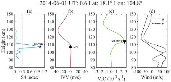
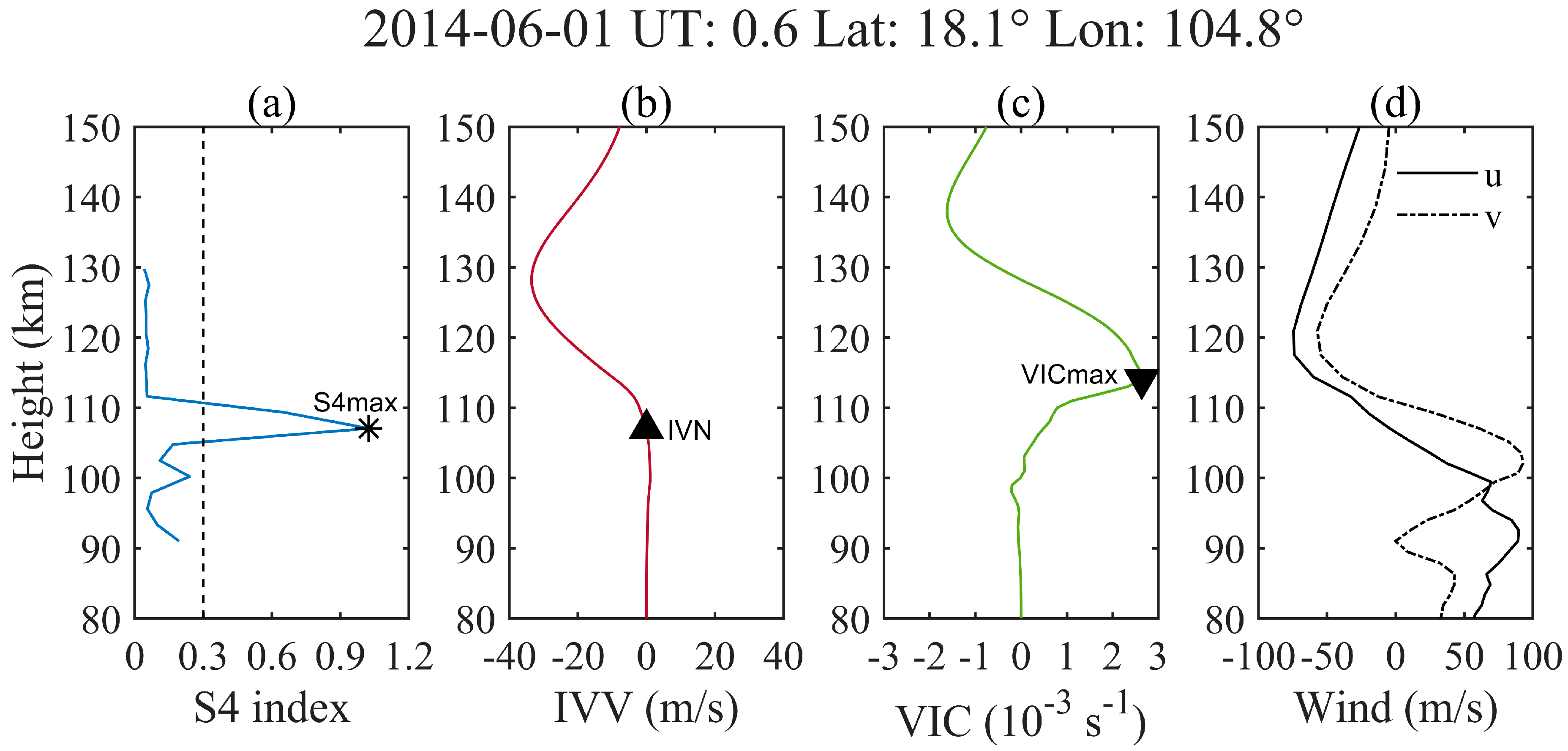
Figure 1.
An example of the sporadic E (Es) layers, ion vertical velocity, and vertical ion convergence (VIC) on 1 June 2014. (a) The blue curve represents the S4 profile. The black dashed curve represents the threshold (S4 > 0.3) that determines Es. The black star represents the S4max; (b) The red curve represents the profile of ion vertical velocity, and the black regular triangle represents the ion vertical velocity null (IVN); (c) The green curve represents the vertical ion convergence (VIC). The black inverted triangle represents the VICmax; (d) The black solid curve represents the zonal wind, and the black dash-dotted curve represents the meridional wind.
Previous studies have employed two main parameters (i.e., the maximum positive value of vertical ion convergence (VICmax) and ion vertical velocity null (IVN)) to assess the height of Es layers [11,12,22,23,24]. The VICmax is the point that has a maximum positive value of vertical ion convergence. The VICmax signifies the altitude of the strongest convergence, where metallic ion velocity changes the fastest. This suggests the potential for a high-density ion layer to swiftly form in this region, making its altitude an accepted proxy for the height of the Es layer in previous studies [11,12]. The results of Chu et al. (2014) showed consistency between the height of Es and VICmax [12]. However, Qiu et al. (2021) highlighted that the heights of Es layers and VICmax are not completely consistent in the Es layer formation process [11].
The ion vertical velocity null (IVN) refers to the point at which ion movement transitions from an upward direction at lower altitudes to a downward direction at higher altitudes. This demarcates the altitude where ions come to a standstill and can also be considered the altitude where Es layers are stationed. Numerical simulations suggested that the height of the Es layer agrees well with the height of the IVN above 110 km [22]. A theoretical study by Dalakishvili et al. (2020) also suggested that the height of the Es layer is in closer proximity to the height of IVN [23]. Tang et al. (2022) verified the role of IVN in the height of Es layers based on the observations of ionosondes and ICON/MIGHT [24].
Previous studies have utilized various parameters from the wind shear theory to quantitatively assess its contribution to sporadic E layers. These investigations have revealed both agreements and discrepancies between wind shear theory and Es layers across different parameters [11,12,19,21,24]. However, most of these studies typically focused on individual parameters. Using the WACCM-X (The Whole Atmosphere Community Climate Model with thermosphere and ionosphere extension) model and COSMIC-1 RO observations, this study reexamines the relationship between VICmax, IVN, and Es layer heights at different seasons and latitudes.
In Section 2.1, the COSMIC data and WACCM-X model are described. Section 2.2 introduces the data analysis methods used in this paper, including the definitions of IVN and VICmax. The statistical results are displayed and discussed in Section 3. Section 4 contains our conclusions.
2. Materials and Methods
2.1. Data and Model
2.1.1. COSMIC-1
The FORMOSAT-3/COSMIC constellation consists of six microsatellites that orbit the Earth at an initial altitude of 800 km. The satellites have been operating since the summer of 2006, and the data set is from November 2006 [25]. The radio occultation technique can provide parameters of the ionosphere, such as total electron content (TEC), electron density, and S4 index. The main advantages of RO measurements are global coverage, high vertical resolution, and avoiding the impact of the troposphere.
The S4 index is the scintillation index, which is measured from the signal-to-noise ratio (SNR) intensity fluctuations of the GPS L1 signal (f = 1.575 MHz). The S4 index typically maintains a low value but experiences a rapid increase when the signal passes ionospheric irregularities. Brahmanandam et al. (2012) introduced the details of the S4 index calculation [26]. The period of the S4 index used in this paper is from January 2014 to December 2014. The successive S4 profiles within the altitude range of 90–130 km were selected in our research.
2.1.2. WACCM-X
WACCM-X is one of the atmosphere components of the Community Earth System Model (CESM) (detailed information can be seen at http://www.cesm.ucar/edu/, accessed on 10 May 2021), developed by the National Center for Atmosphere Research (NCAR). The altitude range of WACCM-X is from the ground to the upper thermosphere (~600 km). The horizontal resolutions of WACCM-X are 1.9° and 2.5° in the meridional and zonal directions, respectively. The model has 126 vertical levels in free-run mode and 145 levels in specified dynamics (SD) mode. The WACCM-X includes the physical processes of WACCM developed by NCAR, a neutral chemistry model for the middle atmosphere, an ion chemistry model for the mesosphere and lower thermosphere regions, ion drag, and auroral processes, parameterizations of extreme ultraviolet heating and infrared transfer under nonlocal thermodynamic equilibrium, and modified parameterizations of gravity wave effects and vertical diffusion. An electrodynamics module, which can self-consistently solve the interactions between electric fields, plasma motions, and neutral winds, was implemented in WACCM-X 2.0. Liu et al. (2010) and Liu et al. (2018) gave detailed descriptions of WACCM-X and its upgrade [27,28].
A transient historical simulation with WACCM-X in the free-running mode for 2014 was conducted. This simulation applied the real value of the Kp index, the Ap index, and the F10.7 solar radio flux. Climate Model Intercomparison Project 6 (CMIP6) provided lower boundary forcings, chemical emissions, and solar radiative and particle [29,30]. The main magnetic field was specified according to the 12th International Geomagnetic Reference Field (IGRF-12) [31]. The thermosphere is a strongly forced system in which small changes in the initial state do not significantly affect the calculated climate of the thermosphere [32], so a single transient historical simulation was used in our investigation. The period of the input data set is from January 2014 to December 2014.
2.2. Data Analysis
2.2.1. Ion Vertical Velocity
In our analysis, we employed hourly outputs of horizontal winds in the mesosphere and lower thermosphere. To facilitate subsequent calculations and analyses, wind data were interpolated into a 1 km altitude grid. The interpolated wind data were then utilized to compute the ion vertical velocity and gradient for Fe+ ions. The vertical velocity of ion (upward is positive) can be expressed as [18]:
where is the collision frequency of ions relative to neutral species, is the ion gyro frequency, and and are given by Nygrén [33]. is the zonal wind (eastward is positive), is the meridional wind (southward is positive), and is the magnetic dip, which is derived from the International Geomagnetic Reference Field (IGRF). Then, the vertical ion convergence can be obtained by [19]:
where is the altitude. Ion will be convergent while is positive.
2.2.2. The Height of Different Parameters
The selection process for determining different parameter heights is illustrated in Figure 1. All results in this paper used the geographic latitude. In Figure 1a, the blue curve represents the S4 index profile, while the black dashed line signifies the threshold for Es identification (S4 index > 0.3) [34]. Once the Es layer is identified, the altitude of the maximum S4 index is designated as the height of the Es layer, denoted by a black star in Figure 1a. Figure 1b depicts the profile of the ion vertical velocity, with the point where ion movement shifts from upward at lower altitudes to downward at higher altitudes defined as the ion vertical velocity null (IVN), marked by a black regular triangle in Figure 1b. Figure 1c displays the profile of the vertical ion convergence; the maximum value of the vertical ion convergence, which is positive, is defined as the maximum of vertical ion convergence (VICmax) and marked as a black inverted triangle in Figure 1c. Figure 1d shows the horizontal wind profiles; the black solid line represents the zonal wind (eastward is positive), and the black dash-dotted line represents the meridional wind (southward is positive).
Figure 1 shows an ideal case. The wind shear regions occur at around 110 km for zonal wind and meridional wind. Both of them make ions convergent at ~110 km according to the wind shear theory [2]. The calculated VIC is positive at ~110 km, causing the ions to converge at this altitude. The IVN and VICmax are located at the wind shear region. In this case, the Es layer is also located at the wind shear region and closer to the height of IVN than VICmax. Besides the vertical wind shear as above, the specific directions and values of horizontal wind can also induce the vertical convergence of ions [23]. Both conditions were considered in this paper by using Equation (1).
2.2.3. The Occurrence Rate of Es and IVN
In this analysis, S4 index profiles of 2014 were utilized to compute the occurrence rate of Es layers. These profiles were categorized into four seasons and 24 local time regions. Subsequently, the data within each region were further divided into a sliding window of 5° latitude by 5 km altitude. Within this window, events with a maximum S4 index greater than 0.3 were identified as Es layers cases. The ratio of the number of Es layer cases to the total number of occultation profiles was designated as the Es occurrence rate (EsOR) [35].
Similarly, the ratio of the number of ion vertical velocity null (IVN) to the total number of grid points of simulation at a fixed height and local time was also calculated and described as the occurrence rate of IVN.
3. Results and Discussion
3.1. Comparison of the Heights of Es Layers and Vertical Ion Convergence Parameters
Figure 2 presents scatter density figures illustrating the relationship between the heights of Es layers and IVN at different latitude zones and seasons. In each subfigure, a regular triangle symbolizes an Es–IVN data point, with color indicating the relative density of points. Every subfigure contains a few to over ten thousand points covered over all longitudes. Additionally, each subfigure in Figure 2 provides the diagonal lines (red dashed lines) and the difference between the heights of Es layers and IVN (red characters, the unit is kilometer). The results reveal that both the heights of Es layers and IVN predominantly center around 90–110 km, which is consistent with previous studies [6,36]. The heights of Es layers tend to be lower than that of IVN by several kilometers, approximately 2–6 km. It is easy to see that most points of Es–IVN center at the diagonal lines, indicating good agreements between the heights of Es layers and IVN at low-latitudes (<20°) and mid-latitudes (20–50°).
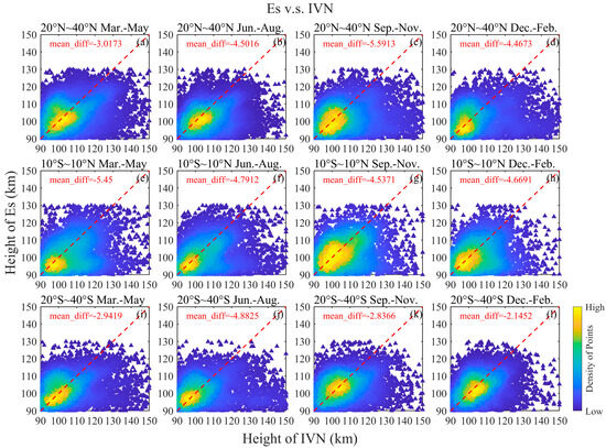
Figure 2.
Scatter density diagram of the height of Es and IVN in the low- and mid-latitudes, 2014. The magenta dashed lines display the diagonals. They represent southern mid-latitude (i–l), low-latitude (e–h), and northern mid-latitude (a–d), respectively, from bottom to top, and represent March–May (a,e,i), June–August (b,f,j), September–November (c,g,k), and December–February (d,h,l), respectively, from left to right.
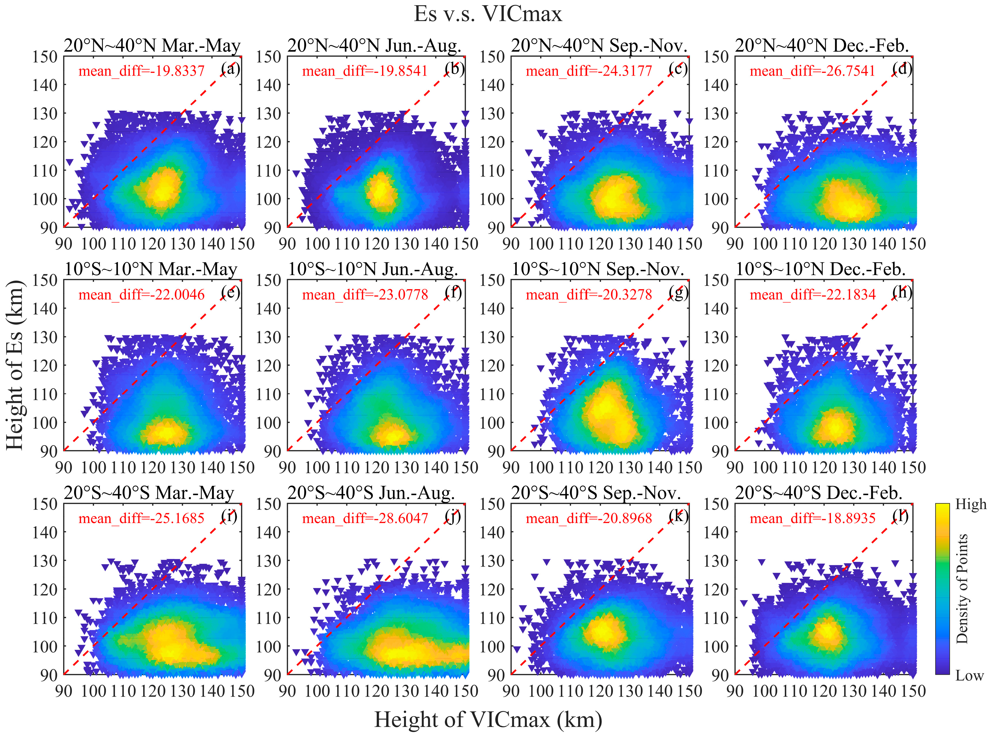
Figure 3 is the same as Figure 2, but inverted triangles in Figure 3 denote data points for Es–VICmax. It is evident from Figure 3 that the height of VICmax predominantly falls within the 110–130 km range, indicating a higher altitude than that of Es layers by approximately 20 km on average at different latitudes and seasons. At the same time, the distributions of the points of Es–VICmax deviate obviously from the diagonal lines at different latitudes and seasons. Upon comparison of the results presented in Figure 2 and Figure 3, it becomes evident that the heights of IVN exhibit stronger agreement with the heights of Es layers observed by COSMIC-1.
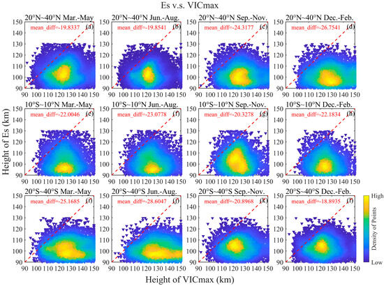
Figure 3.
Scatter density diagram of the height of Es and VICmax in the low- and mid-latitudes, 2014. The magenta dashed lines display the diagonals. They represent southern mid-latitude (i–l), low-latitude (e–h), and northern mid-latitude (a–d), respectively, from bottom to top, and represent March–May (a,e,i), June–August (b,f,j), September–November (c,g,k), and December–February (d,h,l), respectively, from left to right.
For IVN, the vertical ion velocity at this node is zero, resulting in stationary convergent thin layers after Es layer formation. However, the vertical velocity of VICmax may not necessarily be zero. This implies the presence of a thin ion layer undergoing vertical motion, deviating from the height of VICmax. According to the simulation findings [22,23], the Es layer is expected to manifest at the height of IVN. In scenarios where IVN is absent, Es would emerge at the height of VICmax and subsequently move towards a height where both the vertical ion velocity and vertical ion convergence approach zero. Thus, in theory, Es is more closely aligned with the height of IVN. Our results supported this conclusion.
3.2. The Descending Rates of Es Layers and IVN
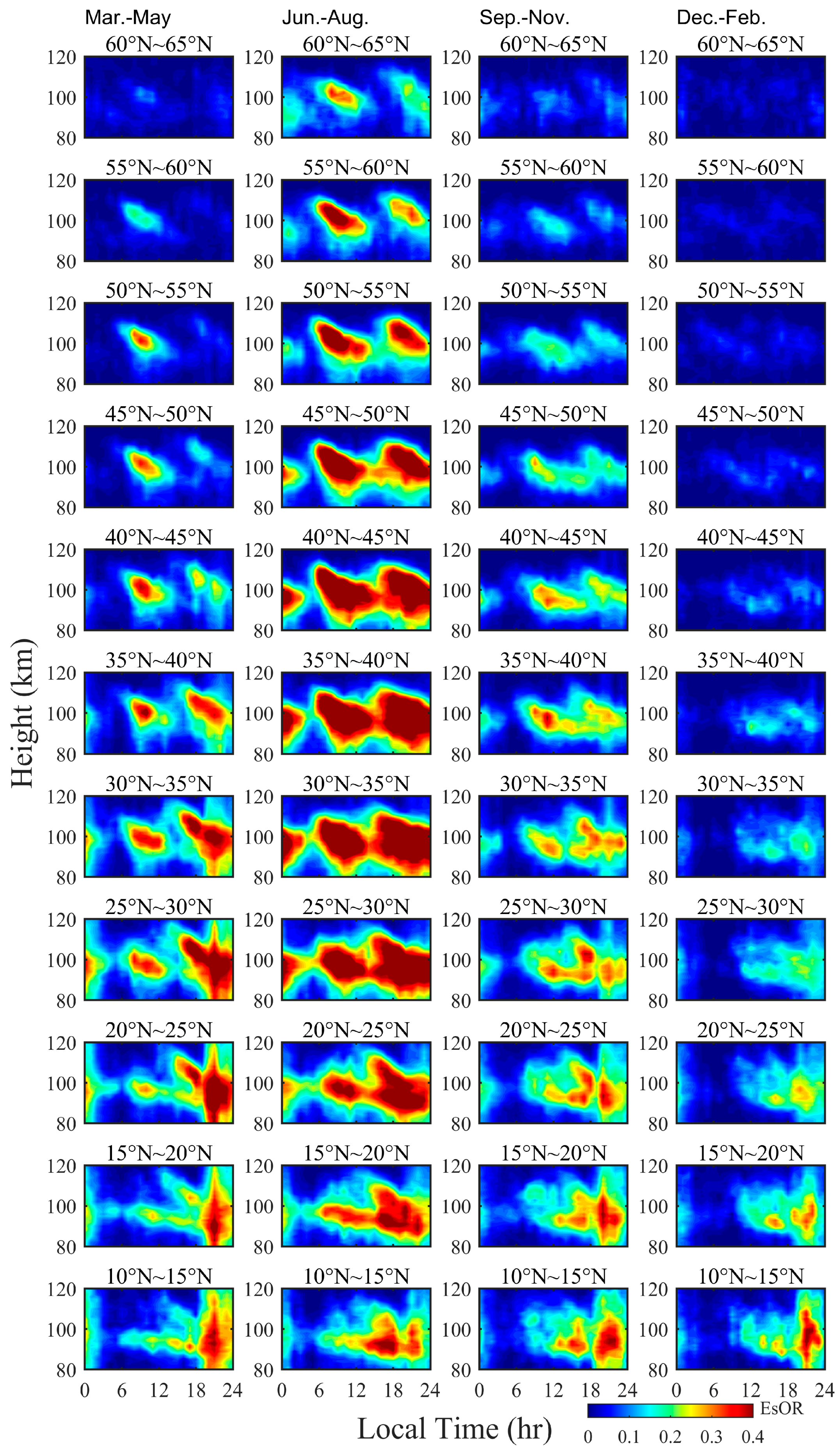
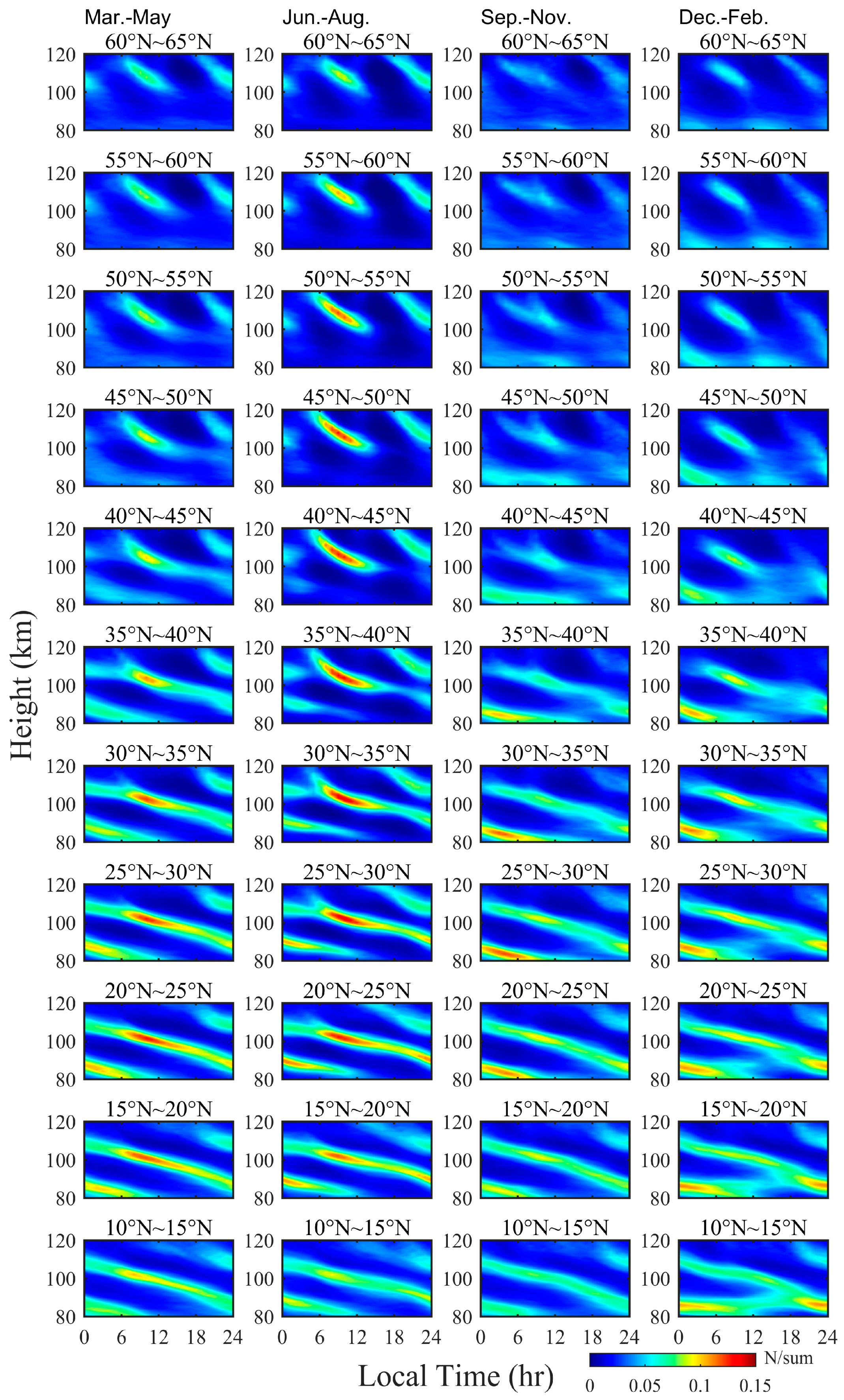
Figure 4 presents the zonal averaged height–local time distributions of EsOR at different latitudes and seasons, derived from the S4 index data of COSMIC-1. The height of the most Es occurrence is from ~110 km to ~95 km, with local time at mid-latitude. Notably, there is a clear seasonal pattern observed through horizontal comparison. Es layers are predominantly observed in summer, with rare occurrences in winter. Additionally, Figure 4 illustrates the diurnal and semidiurnal variations in EsOR and the corresponding heights. The diurnal variation prevails at lower latitudes, while the semidiurnal variation takes precedence at mid-latitudes. These findings align with prior research, attributing these patterns to the influence of tides on neutral horizontal winds [7,12,15,37].
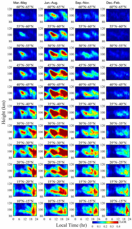
Figure 4.
Local time–height distributions of EsOR of the northern hemisphere in different seasons and latitudes of 2014, representing low latitude to high latitude from bottom to top for spring (March–May), summer (June–August), autumn (September–November), and winter (December–February), respectively, from left to right.
Simultaneously, Figure 5 illustrates the zonal averaged height–local time distributions of the IVN occurrence rate, calculated from the WACCM-X wind data. The height of the most IVN occurrence is from less than 120 km to ~97 km with local time at mid-latitude. IVN tends to occur more frequently in summer compared to other seasons. Similarly, diurnal and semidiurnal variations, along with their latitudinal distributions, can be discerned in the height variation and occurrence rate of IVN. These findings highlight the consistency between the variations in IVN height and Es occurrence.
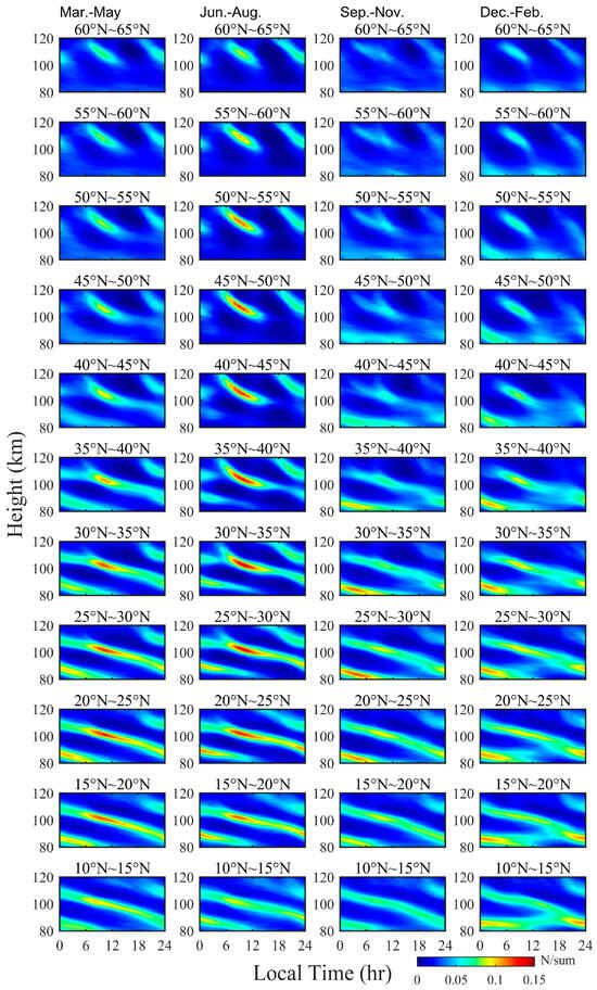
Figure 5.
Local time–height distributions of the occurrence rate of IVN of the northern hemisphere in different seasons and latitudes of 2014, representing low latitude to high latitude from bottom to top for spring (March–May), summer (June–August), autumn (September–November), and winter (December–February), respectively, from left to right.
The results of this study suggest that Es layers occur at the height of IVN and are dragged down by IVN, aligning with the results reported by Qiu [22]. Simulation studies propose that a thin, high-density metal ion layer, generated under the wind shear theory, stabilizes at roughly the height of IVN within thirty minutes [22,23]. It is worth noting that Es layers will be stationary while Es layers are down below 100 km in Figure 4. However, the descent of IVN is continued in Figure 5. Qiu et al. (2023) and Tang et al. (2023) reported a similar phenomenon; they attributed the phenomenon to that of the gradient of the ratio of the ion-neutral collision frequency to the ion gyrofrequency, which plays an important role in the formation of the Es layers at a lower altitude [22,24]. The height–local time distributions of the southern hemisphere and near-equatorial regions show the same result as above and are displayed in Figures S1–S4 of Supplementary Materials.
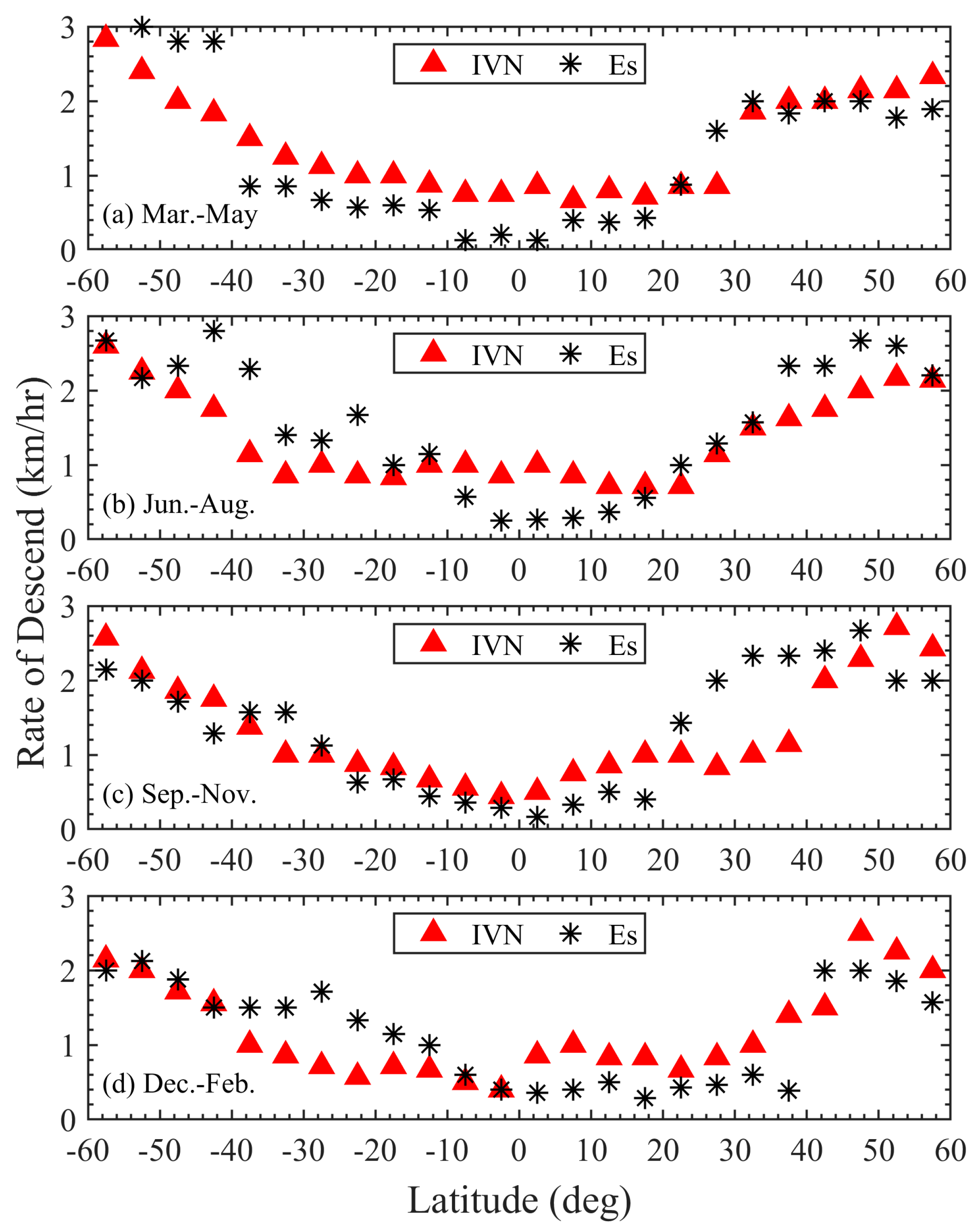
Furthermore, the descent rates of both IVN and Es layers were estimated based on their height–local time distributions. Figure 6 illustrates the descent rates of Es and IVN at different latitudes. In low- and mid-latitudes, the descent rates of Es layers range from 0.25 to 3 km/h. As latitude increases, the rate of Es descent will gradually increase. This trend is separated into two phases: the descent rate is below 1 km/h at below ~30 degrees; the descent rate is 1–3 km/h and increases faster at above 30 degrees than that of below ~30 degrees. This pattern aligns with the latitudinal distribution of IVN’s descent rate. This is due to the dominance of diurnal and semidiurnal tides at low- and mid-latitudes, respectively [38]. Notably, previous studies considered VICmax as the height of Es layers. However, this paper suggests that IVN can better represent the height variations of Es layers.

Figure 6.
Estimated descent rates of IVN and Es in the low- and mid-latitudes for (a) March–May, (b) June–August, (c) September–November, and (d) December–February.
Besides the atmospheric tides of the horizontal winds, some factors also play roles in the formation and development of the Es layers (i.e., the electric fields, the diffusion, the atmospheric gravity waves, the collision frequency of ions relative to neutral species, and so on) [23,24,39,40,41,42,43]. According to the results of Resende et al. (2016) and Cai et al. (2019), the electric field suppresses the occurrence of the Es layers in the daytime in equatorial regions [39,40]. The diffusion suppresses occurrence and accelerates dissipation for the Es layer [23,40]. At the same time, the atmospheric gravity waves contribute to the small-scale structures of the Es layers based on the simulations of Cai et al. (2017) and Qiu et al. (2023) [41,42], and may induce the formation of the multilayered sporadic E based on the result of Didebulidze et al. (2020) [43]. The enhancement of collision frequency induces the Es layers to separate with IVN in the vertical direction below the altitude of 110 km [24]. Additionally, a 3D simulation of Andoh et al. (2023) displayed the horizontal movement of Es driven by the horizontal transport of ions [44]. In the future, those processes need to be taken into account in our research with further study on the Es layers.
4. Conclusions
This study compared the heights between Es layers and IVN and VICmax, using the WACCM-X model and COSMIC-1 RO observations for the period from January 2014 to December 2014. The main findings can be summarized as follows:
- IVN proves to be a more suitable parameter for accurately representing the height of Es layers;
- The descents of ion vertical velocity null agree well with that of Es layers at different latitudes.
Supplementary Materials
The following supporting information can be downloaded at: https://www.mdpi.com/article/10.3390/rs15245674/s1, Figure S1: Local time–height distributions of EsOR with equatorial regions in different seasons and latitudes of 2014; Figure S2: Local time–height distributions of the occurrence rate of IVN with equatorial regions in different seasons and latitudes of 2014; Figure S3: Local time–height distributions of EsOR of the southern hemisphere in different seasons and latitudes of 2014; Figure S4: Local time–height distributions of the occurrence rate of IVN of the southern hemisphere in different seasons and latitudes of 2014.
Author Contributions
Conceptualization, Y.Y. and L.Q.; methodology, Y.Q. and Y.Y.; validation, L.Q.; data curation, Y.Q.; visualization, Y.Y. and Y.L.; writing—original draft preparation, Y.Y.; writing—review and editing, L.Q., S.L. and T.Y.; supervision, J.W. and T.Y.; project administration, X.Y. and T.Y.; funding acquisition, T.Y. and X.Y. All authors have read and agreed to the published version of the manuscript.
Funding
This research was funded by the National Natural Science Foundation of China (grant no: 42230207, 42074191).
Data Availability Statement
Data are contained within the article and Supplementary Materials.
Acknowledgments
The WACCM-X model source code can be found at (https://www2.hao.ucar.edu/modeling/waccm-x, accessed on 10 May 2021). The F3/C data were provided by the COSMIC Data Analysis and Archival Center and the Taiwan Analysis Center for COSMIC (https://cdaac-www.cosmic.ucar.edu/, accessed on 20 August 2018).
Conflicts of Interest
The authors declare no conflict of interest.
References
- Qiu, L.; Yu, T.; Yan, X.; Sun, Y.; Zuo, X.; Yang, N.; Wang, J.; Qi, Y. Altitudinal and Latitudinal Variations in Ionospheric Sporadic-E Layer Obtained From FORMOSAT-3/COSMIC Radio Occultation. JGR Space Phys. 2021, 126, e2021JA029454. [Google Scholar] [CrossRef]
- Haldoupis, C. A Tutorial Review on Sporadic E Layers. In Aeronomy of the Earth’s Atmosphere and Ionosphere; Abdu, M.A., Pancheva, D., Eds.; Springer: Dordrecht, The Netherlands, 2011; pp. 381–394. [Google Scholar] [CrossRef]
- Yue, X.; Schreiner, W.S.; Pedatella, N.M.; Kuo, Y. Characterizing GPS Radio Occultation Loss of Lock Due to Ionospheric Weather. Space Weather 2016, 14, 285–299. [Google Scholar] [CrossRef]
- Hosokawa, K.; Kimura, K.; Sakai, J.; Saito, S.; Tomizawa, I.; Nishioka, M.; Tsugawa, T.; Ishii, M. Visualizing Sporadic E Using Aeronautical Navigation Signals at VHF Frequencies. J. Space Weather Space Clim. 2021, 11, 6. [Google Scholar] [CrossRef]
- Haldoupis, C.; Meek, C.; Christakis, N.; Pancheva, D.; Bourdillon, A. Ionogram Height–Time–Intensity Observations of Descending Sporadic E Layers at Mid-Latitude. J. Atmos. Sol. Terr. Phys. 2006, 68, 539–557. [Google Scholar] [CrossRef]
- Arras, C.; Wickert, J.; Beyerle, G.; Heise, S.; Schmidt, T.; Jacobi, C. A Global Climatology of Ionospheric Irregularities Derived from GPS Radio Occultation. Geophys. Res. Lett. 2008, 35, L14809. [Google Scholar] [CrossRef]
- Christakis, N.; Haldoupis, C.; Zhou, Q.; Meek, C. Seasonal Variability and Descent of Mid-Latitude Sporadic E Layers at Arecibo. Ann. Geophys. 2009, 27, 923–931. [Google Scholar] [CrossRef]
- Maeda, J.; Heki, K. Morphology and Dynamics of Daytime Mid-Latitude Sporadic-E Patches Revealed by GPS Total Electron Content Observations in Japan. Earth Planets Space 2015, 67, 89. [Google Scholar] [CrossRef]
- Arras, C.; Wickert, J. Estimation of Ionospheric Sporadic E Intensities from GPS Radio Occultation Measurements. J. Atmos. Sol. Terr. Phys. 2018, 171, 60–63. [Google Scholar] [CrossRef]
- Yu, B.; Xue, X.; Yue, X.; Yang, C.; Yu, C.; Dou, X.; Ning, B.; Hu, L. The Global Climatology of the Intensity of the Ionospheric Sporadic E Layer. Atmos. Chem. Phys. 2019, 19, 4139–4151. [Google Scholar] [CrossRef]
- Qiu, L.; Zuo, X.; Yu, T.; Sun, Y.; Liu, H.; Sun, L.; Zhao, B. The Characteristics of Summer Descending Sporadic E Layer Observed with the Ionosondes in the China Region. JGR Space Phys. 2021, 126, e2020JA028729. [Google Scholar] [CrossRef]
- Chu, Y.H.; Wang, C.Y.; Wu, K.H.; Chen, K.T.; Tzeng, K.J.; Su, C.L.; Feng, W.; Plane, J.M.C. Morphology of Sporadic E Layer Retrieved from COSMIC GPS Radio Occultation Measurements: Wind Shear Theory Examination. J. Geophys. Res. Space Phys. 2014, 119, 2117–2136. [Google Scholar] [CrossRef]
- Haldoupis, C.; Pancheva, D. Terdiurnal Tidelike Variability in Sporadic E Layers. J. Geophys. Res. 2006, 111, A07303. [Google Scholar] [CrossRef]
- Šauli, P.; Bourdillon, A. Height and Critical Frequency Variations of the Sporadic-E Layer at Midlatitudes. J. Atmos. Sol. Terr. Phys. 2008, 70, 1904–1910. [Google Scholar] [CrossRef]
- Tang, Q.; Zhou, C.; Liu, H.; Du, Z.; Liu, Y.; Zhao, J.; Yu, Z.; Zhao, Z.; Feng, X. Global Structure and Seasonal Variations of the Tidal Amplitude in Sporadic-E Layer. JGR Space Phys. 2022, 127, e2022JA030711. [Google Scholar] [CrossRef]
- Zuo, X.; Wan, W. Planetary Wave Oscillations in Sporadic E Layer Occurrence at Wuhan. Earth Planets Space 2008, 60, 647–652. [Google Scholar] [CrossRef]
- Jacobi, C.; Arras, C. Tidal Wind Shear Observed by Meteor Radar and Comparison with Sporadic E Occurrence Rates Based on GPS Radio Occultation Observations. Adv. Radio Sci. 2019, 17, 213–224. [Google Scholar] [CrossRef]
- Whitehead, J.D. Formation of the Sporadic E Layer in the Temperate Zones. Nature 1960, 188, 567. [Google Scholar] [CrossRef]
- Shinagawa, H.; Miyoshi, Y.; Jin, H.; Fujiwara, H. Global Distribution of Neutral Wind Shear Associated with Sporadic E Layers Derived from GAIA. J. Geophys. Res. Space Phys. 2017, 122, 4450–4465. [Google Scholar] [CrossRef]
- Qiu, L.; Zuo, X.; Yu, T.; Sun, Y.; Qi, Y. Comparison of Global Morphologies of Vertical Ion Convergence and Sporadic E Occurrence Rate. Adv. Space Res. 2019, 63, 3606–3611. [Google Scholar] [CrossRef]
- Yamazaki, Y.; Arras, C.; Andoh, S.; Miyoshi, Y.; Shinagawa, H.; Harding, B.J.; Englert, C.R.; Immel, T.J.; Sobhkhiz-Miandehi, S.; Stolle, C. Examining the Wind Shear Theory of Sporadic E With ICON/MIGHTI Winds and COSMIC-2 Radio Occultation Data. Geophys. Res. Lett. 2022, 49, e2021GL096202. [Google Scholar] [CrossRef]
- Qiu, L.; Yamazaki, Y.; Yu, T.; Miyoshi, Y.; Zuo, X. Numerical Investigation on the Height and Intensity Variations of Sporadic E Layers at Mid-Latitude. JGR Space Phys. 2023, 128, e2023JA031508. [Google Scholar] [CrossRef]
- Dalakishvili, G.; Didebulidze, G.G.; Todua, M. Formation of Sporadic E (Es) Layer by Homogeneous and Inhomogeneous Horizontal Winds. J. Atmos. Sol. Terr. Phys. 2020, 209, 105403. [Google Scholar] [CrossRef]
- Tang, Q.; Zhou, C.; Liu, H.; Liu, Y.; Zhao, J.; Yu, Z.; Hu, L.; Zhao, Z.; Feng, X. Low Altitude Tailing Es (LATTE): Analysis of Sporadic-E Layer Height at Different Latitudes of Middle and Low Region. Space Weather 2023, 21, e2022SW003323. [Google Scholar] [CrossRef]
- Anthes, R.A.; Bernhardt, P.A.; Chen, Y.; Cucurull, L.; Dymond, K.F.; Ector, D.; Healy, S.B.; Ho, S.-P.; Hunt, D.C.; Kuo, Y.-H.; et al. The COSMIC/FORMOSAT-3 Mission: Early Results. Bull. Amer. Meteor. Soc. 2008, 89, 313–334. [Google Scholar] [CrossRef]
- Brahmanandam, P.S.; Uma, G.; Liu, J.Y.; Chu, Y.H.; Latha Devi, N.S.M.P.; Kakinami, Y. Global S4 Index Variations Observed Using FORMOSAT-3/COSMIC GPS RO Technique during a Solar Minimum Year: GLOBAL S4 INDEX MAPS. J. Geophys. Res. 2012, 117, A9. [Google Scholar] [CrossRef]
- Liu, H.-L.; Foster, B.T.; Hagan, M.E.; McInerney, J.M.; Maute, A.; Qian, L.; Richmond, A.D.; Roble, R.G.; Solomon, S.C.; Garcia, R.R.; et al. Thermosphere Extension of the Whole Atmosphere Community Climate Model: Whole atmosphere model. J. Geophys. Res. 2010, 115, A12302. [Google Scholar] [CrossRef]
- Liu, H.; Bardeen, C.G.; Foster, B.T.; Lauritzen, P.; Liu, J.; Lu, G.; Marsh, D.R.; Maute, A.; McInerney, J.M.; Pedatella, N.M.; et al. Development and Validation of the Whole Atmosphere Community Climate Model with Thermosphere and Ionosphere Extension (WACCM-X 2.0). J. Adv. Model Earth Syst. 2018, 10, 381–402. [Google Scholar] [CrossRef]
- Eyring, V.; Bony, S.; Meehl, G.A.; Senior, C.A.; Stevens, B.; Stouffer, R.J.; Taylor, K.E. Overview of the Coupled Model Intercomparison Project Phase 6 (CMIP6) Experimental Design and Organization. Geosci. Model Dev. 2016, 9, 1937–1958. [Google Scholar] [CrossRef]
- Matthes, K.; Funke, B.; Andersson, M.E.; Barnard, L.; Beer, J.; Charbonneau, P.; Clilverd, M.A.; Dudok de Wit, T.; Haberreiter, M.; Hendry, A.; et al. Solar Forcing for CMIP6 (v3.2). Geosci. Model Dev. 2017, 10, 2247–2302. [Google Scholar] [CrossRef]
- Thébault, E.; Finlay, C.C.; Beggan, C.D.; Alken, P.; Aubert, J.; Barrois, O.; Bertrand, F.; Bondar, T.; Boness, A.; Brocco, L.; et al. International Geomagnetic Reference Field: The 12th Generation. Earth Planets Space 2015, 67, 79. [Google Scholar] [CrossRef]
- Codrescu, S.M.; Codrescu, M.V.; Fedrizzi, M. An Ensemble Kalman Filter for the Thermosphere-Ionosphere. Space Weather 2018, 16, 57–68. [Google Scholar] [CrossRef]
- Nygrén, T.; Jalonen, L.; Oksman, J.; Turunen, T. The Role of Electric Field and Neutral Wind Direction in the Formation of Sporadic E-Layers. J. Atmos. Terr. Phys. 1984, 46, 373–381. [Google Scholar] [CrossRef]
- Yue, X.; Schreiner, W.S.; Zeng, Z.; Kuo, Y.-H.; Xue, X. Case Study on Complex Sporadic E Layers Observed by GPS Radio Occultations. Atmos. Meas. Tech. 2015, 8, 225–236. [Google Scholar] [CrossRef]
- Arras, C.; Wickert, J.; Jacobi, C.; Beyerle, G.; Heise, S.; Schmidt, T. Global Sporadic E Layer Characteristics Obtained from GPS Radio Occultation Measurements. In Climate and Weather of the Sun-Earth System (CAWSES); Lübken, F.-J., Ed.; Springer Atmospheric Sciences; Springer: Dordrecht, The Netherlands, 2013; pp. 207–221. [Google Scholar] [CrossRef]
- Bishop, R.L.; Earle, G.D.; Larsen, M.F.; Swenson, C.M.; Carlson, C.G.; Roddy, P.A.; Fish, C.; Bullett, T.W. Sequential Observations of the Local Neutral Wind Field Structure Associated with E Region Plasma Layers: E region layers and local neutral wind field. J. Geophys. Res. 2005, 110, A4. [Google Scholar] [CrossRef]
- Zhou, C.; Tang, Q.; Song, X.; Qing, H.; Liu, Y.; Wang, X.; Gu, X.; Ni, B.; Zhao, Z. A Statistical Analysis of Sporadic E Layer Occurrence in the Midlatitude China Region. J. Geophys. Res. Space Physics 2017, 122, 3617–3631. [Google Scholar] [CrossRef]
- Yu, Y.; Wan, W.; Ren, Z.; Xiong, B.; Zhang, Y.; Hu, L.; Ning, B.; Liu, L. Seasonal Variations of MLT Tides Revealed by a Meteor Radar Chain Based on Hough Mode Decomposition. JGR Space Phys. 2015, 120, 7030–7048. [Google Scholar] [CrossRef]
- Resende, L.C.A.; Batista, I.S.; Denardini, C.M.; Carrasco, A.J.; De Fátima Andrioli, V.; Moro, J.; Batista, P.P.; Chen, S.S. Competition between Winds and Electric Fields in the Formation of Blanketing Sporadic E Layers at Equatorial Regions. Earth Planets Space 2016, 68, 201. [Google Scholar] [CrossRef]
- Cai, X.; Yuan, T.; Eccles, J.V.; Pedatella, N.M.; Xi, X.; Ban, C.; Liu, A.Z. A Numerical Investigation on the Variation of Sodium Ion and Observed Thermospheric Sodium Layer at Cerro Pachón, Chile during Equinox. JGR Space Phys. 2019, 124, 10395–10414. [Google Scholar] [CrossRef]
- Cai, X.; Yuan, T.; Eccles, J.V. A Numerical Investigation on Tidal and Gravity Wave Contributions to the Summer Time Na Variations in the Midlatitude E Region. J. Geophys. Res. Space Phys. 2017, 122, 10577–10595. [Google Scholar] [CrossRef]
- Qiu, L.; Yamazaki, Y.; Yu, T.; Becker, E.; Miyoshi, Y.; Qi, Y.; Siddiqui, T.A.; Stolle, C.; Feng, W.; Plane, J.M.C.; et al. Numerical Simulations of Metallic Ion Density Perturbations in Sporadic E Layers Caused by Gravity Waves. Earth Space Sci. 2023, 10, e2023EA003030. [Google Scholar] [CrossRef]
- Didebulidze, G.G.; Dalakishvili, G.; Todua, M. Formation of Multilayered Sporadic E under an Influence of Atmospheric Gravity Waves (AGWs). Atmosphere 2020, 11, 653. [Google Scholar] [CrossRef]
- Andoh, S.; Saito, A.; Shinagawa, H. Simulation of Horizontal Sporadic E Layer Movement Driven by Atmospheric Tides. Earth Planets Space 2023, 75, 86. [Google Scholar] [CrossRef]

Disclaimer/Publisher’s Note: The statements, opinions and data contained in all publications are solely those of the individual author(s) and contributor(s) and not of MDPI and/or the editor(s). MDPI and/or the editor(s) disclaim responsibility for any injury to people or property resulting from any ideas, methods, instructions or products referred to in the content. |
© 2023 by the authors. Licensee MDPI, Basel, Switzerland. This article is an open access article distributed under the terms and conditions of the Creative Commons Attribution (CC BY) license (https://creativecommons.org/licenses/by/4.0/).