Adaptive Space–Location-Weighting Function Method for High-Precision Density Inversion of Gravity Data

Abstract

Underground 3D density variation can be obtained via the inversion of gravity data, which is a very important basis for structural division, oil and gas structure definition, and mineral resource evaluation. A depth-weighting function is usually introduced as a structural constraint in density inversion to solve the skin effect. We propose an adaptive space–location-weighting (ASW) function for gravity field data to improve the resolution of the inversion, which adds the position and depth information provided by the DEXP method to form a new weighting function. The weighting function is partitioned according to the horizontal distribution of the source and can effectively improve the resolution of field sources with different positions and different depths. The results of model tests have shown that the ASW function method can significantly improve the precision and resolution of density inversion results and has good noise immunity. The ASW method was applied to interpret the real gravity data of a mining area in Shandong, and we speculated potential mineralization based on the inversion results, which corresponded well with the logging results.

1. Introduction

Gravity exploration, as an essential exploration method for remote sensing measurement [1], can effectively obtain comprehensive responses to an irregular underground density distribution [2]. With the advantages of high efficiency, low cost, and a wide range, it has been widely applied in metallogenic prospect prediction, as well as oil, gas, and mineral resource exploration [3]. The physical property inversion method calculates the density parameter of a field source by solving the optimization problem of the equation for physical property parameters and observed anomalies. Higher precision inversion is favorable to a more accurate estimation of underground mineral distribution and geological structure. Therefore, improving the space resolution of inversion results has become a hot topic in research.

Last and Kubik [4] proposed a focused inversion method in which inversion precision was improved through the addition of prior information as a restriction. The inversion results were more in line with actual geological conditions. Barbosa [5] has given a direction in which the inversion process can be focused. Li [6] added the orientation and inclination data of the geological body to the objective function to improve the resolution of the inversion results of known inclination information conditions. The addition of different geophysical data or geological information can also increase the anomaly information to obtain more accurate density inversion results. For example, the cross-gradient method has been used to perform joint inversion of gravity and magnetic data, more accurately with the same field sources [7]. Cai et al. [8] added a gradient component and applied a normalized property-weighting function by using a cross-gradient that can effectively improve the resolution of inversion results. Meng et al. [9] divided the underground into an unstructured grid and proposed the second-order Taylor formula cross-gradient method to perform the joint inversion of gravity and magnetic data, which could better fit the boundaries of irregular geological bodies.

The kernel function of gravity rapidly decays with increasing depths, which causes density inversion results to be concentrated close to the ground and reduces vertical resolution. One important way to improve this resolution is to establish a depth-weighting function and add it to the objective function. Many scholars have proposed different depth-weighting function forms. In particular, the depth-weighting function proposed by Li and Oldenburg [10] has been widely used in potential field inversion. Later, scholars improved this function. Boulanger [11] used the Lagrangian formula to combine different weights and compare the effects thereof. Commer [12] proposed a depth-weighting function based on the depth of the top surface of the geological body, which could obtain accurate inversion results. This function was improved to be more accurate in recognizing the range of preset parameters and the location of the filed sources [13]. Imposing hard constraints on physical bounds is essential to recovering a geologically plausible model [14]. Yang et al. [15] introduced exponential depth-weighting functions to perform the individual and joint focus inversion of some gravitational gradient tensor components, achieving good results. In addition, Qin et al. [16] estimate the depth of the anomalous body by single component inversion, and the depth information is incorporated into the depth-weighting function. Cella and Fedi [17] assumed that the exponent of a depth-weighting function correlates with the field attenuation of the entire source, which has better objectivity. Vitale and Fedi [18] extended this hypothesis to fields with complex structures and obtained depth-weighted indices from multi-scale field uniformity estimates. Gebre et al. [19] proposed a new depth-weighting function that can automatically determine the value of the β parameter using standard optimization methods. A spherical coordinate inversion method based on hybrid regularization and the depth-weighting function has also been put forward [20].

By adding a prior information constraint, using a joint inversion method, and introducing a weighting function, there has been an improvement in the resolution of the inversion. However, due to the local optimization of the algorithm, the recovery of field sources at deeper depths still needs to be improved, especially in the event of the existence of multiple geological bodies at different depths. To improve the resolution of the density inversion of gravity data, we propose the adaptive space–location-weighting (ASW) function method. It uses location information provided by the Depth from Extreme Points (DEXP) method [21] to adaptively design a weighting function. The ASW function can effectively balance the amplitude differences of sources with different depths to obtain higher-resolution results. The advantages of this method were tested on theoretical models and compared to the inversion method with the depth-weighting function. Finally, the real measured data of a mining area in Shandong were used to verify the practicability of the ASW function method.

2. Methodology

The density inversion of gravity data generally involves dividing underground space into regular prismatic units of the same size, in which a linear relationship can be observed between the gravity anomaly $d$ and the residual density $\rho$. It can be given as follows:

$$d=G\rho$$

(1)

where the kernel function, $G$, represents the sensitivity matrix. Inversion is the process of solving the optimal solution of an objective function. The inversion problem is commonly converted to the issue of solving the optimal solution of the objective function. Since inversion is an underdetermined problem, a stable unique solution cannot be obtained by directly solving the optimization problem of the equation, and additional constraints need to be added to obtain a reasonable inversion result. The noise components contained in observed data will also interfere with the inversion process. The Tikhonov regularization method is usually introduced to solve these problems and improve inversion stability [22]. After the regularization of the minimal model constraint is added, the objective function can be expressed as follows:

$$\varphi ={‖\left(G\rho -d\right)‖}_2^2+\alpha {‖W_z\rho ‖}_2^2$$

(2)

where $\alpha$ is the regularization parameter that is given by the L-curve method [22], and $W_z$ is the depth-weighting function proposed by Li and Oldenburg [23]. It is established to offset the attenuation effect of the kernel function, thereby enhancing the vertical resolution of the data. Its diagonal element expression is as follows:

$$W_z=\frac{1}{{\left(z+z_0\right)}^{\frac{\beta }{2}}}$$

(3)

where $z$ is the depth of the center point of the grid element, and $z_0$ is a constant that depends on the cell size of the model discretization and the observation height of the data. $\beta$ is a constant that is equal to 2 for gravity data [23].

The depth-weighting function $W_z$ is only depth-dependent, which does not contain the depth information of the source; therefore, the vertical resolution of the inversion is low. To improve the precision of the inversion, we established a new weighted function $W_{\Omega }$. It can effectively reflect the field source characteristics at different depths and locations. It can be expressed as follows:

$$W_{\Omega }={\left(\frac{\Omega }{{\left|\Omega \right|}_{\max }}\right)}^{\gamma }$$

(4)

where $\Omega$ is a matrix of field sources position information. $\gamma$ is a weight coefficient, and the range of which was determined to be 0–1. The selection of the value for $\gamma$ will be discussed in detail in the subsequent model tests. Rapid imaging technology does not require iteration and therefore can quickly provide relevant parameters, such as the location distribution and physical properties of sources. Thus, we selected the automatic DEXP imaging [21] to obtain the space information $\Omega$ that is contained in $W_{\Omega }$ and established as follows:

$$\Omega =h_i{}^{\frac{-1}{2}}\frac{f_1}{f_2}$$

(5)

where $h_i$ is the height of the upward continuation, and $f_1$ and $f_2$ are the first- and second-order vertical derivatives of the gravity anomaly $d$ with different heights. The $f_1$ and $f_2$ are obtained by the multi-layer equivalent source method, which is a stable computation way [24].

The parameters of the multi-layer equivalent source are determined from the spectral characteristics of the data. The Fourier transform is performed on the measured anomaly and the power spectrum is calculated. The power spectrum function P at any depth h can be written as follows:

$$P=l{\exp }^{-2rh}$$

(6)

where $l$ is a constant related to the physical properties of the geological body, and $r=\sqrt{u^2+v^2}$ is the radial circular frequency associated with $u$ and $v$. We take the logarithm of Equation (6) on both sides:

$$\ln P=\ln l-2hr$$

(7)

We calculate the slope of the power spectrum curve, which gives the average depth of the equivalent layer. By analyzing the spectral characteristics of the anomaly, the number of equivalent layers is determined from the shape of this curve as $n$. Performing segmented fitting, we calculate the average depth $h_k$ of the equivalent layer for the $k$-th layer and extract the anomaly $d_k$ of the equivalent layer for the $k$-th layer. The observed anomaly, denoted as $d$, can be expressed as follows:

$$d={\displaystyle \sum _{k=1}^n{d}_k+e}$$

(8)

In order to effectively balance the impact of the thickness of each equivalent layer on data fitting, the thickness of each equivalent layer is determined by the ratio of the mean total horizontal derivative (MTHD) of the separated anomaly $d_k$ at each layer. Horizontal directional derivatives are a commonly used gradient-based filter for enhancing linear features in potential field data [25]. The mean total horizontal derivative for the $k$-th layer anomaly (MTHD_k) can be expressed as follows:

$$MTH{D}_k=\frac{1}{Mi}{\displaystyle \sum _{i=1}^{Mi}\sqrt{{\left(\frac{\partial d_{k_i}}{\partial x}\right)}^2+{\left(\frac{\partial d_{k_i}}{\partial y}\right)}^2}}$$

(9)

where $M_i$ denotes the number of observation points, and $d_{k_i}$ represents the $i$-th observed value of $d_k$. Acknowledging the influence of high-frequency noise within the separated anomaly of the first layer, we opt to employ the second layer’s mean total horizontal derivative (MTHD₂) as a benchmark. Consequently, the thickness ratio for the $k$-th layer is determined as follows:

$$R_k=MTH{D}_k/MTH{D}_2$$

(10)

Assuming the average sampling interval is $dx$, the thickness of the $k$-th layer is as follows:

$$T_k=dx\cdot R_k$$

(11)

The calculation of multi-layer equivalent sources resembles three-dimensional physical property inversion. Combined with the anomaly $d_k$ of each layer separated by the spectral analysis, we calculate the kernel function matrix applicable to the different equivalent layers for solving the equivalent physical property parameters of each layer. Therefore, we construct the kernel function $G_k$ of the $k$th layer’s equivalent source in the observation surface with the calculated layer depth $h_k$ and thickness of the $k$th layer. Combined with Formula (1), the correspondence between the anomaly data of each layer and the equivalent layer is as follows:

$$d_k=G_k{m}_k$$

(12)

where $m_k$ is the physical parameter of the $k$th layer equivalent source. Combining with Formula (8), the multilayer equivalent source can be expressed as follows:

$$d_{inv}={\displaystyle \sum _{k=1}^n{G}_k{m}_k}$$

(13)

where $d_{inv}$ is the reversion result of the multi-layer equivalent sources at the original observation position. Therefore, we can also perform forward modeling based on the equivalent source physical parameters to obtain the first- and second-order vertical derivatives of the gravity anomaly at different heights, which are $f_1$ and $f_2$.

However, inversion is a process of local optimization. When multiple field sources with different depths are in the same space, the inversion results of the deeper sources will be largely influenced by the shallower sources. This will better reflect the characteristics of the shallower field sources, while the recovery of deep field-source amplitude will not be good. Therefore, we partitioned the inversion space to calculate different depth field sources in different regions, and the improved combination of positional weights in the partitioned space is as follows:

$$W_{\Omega }\prime =\left[\begin{array}{cccc}{W}_{{\Omega }_1}& & & \\ & W_{{\Omega }_2}& & \\ & & \ddots & \\ & & & W_{{\Omega }_i}\end{array}\right]$$

(14)

where $W_{{\Omega }_i}$ represents the value of the internal weighting function of the divided subregion, and it can be expressed as follows:

$$W_{{\Omega }_i}={\left(\frac{{\Omega }_i}{{\left|{\Omega }_i\right|}_{\max }}\right)}^{\gamma }$$

(15)

The ASW expression can be given as follows:

$$\varphi ={‖W_d\left(G\rho -d\right)‖}_2^2+\alpha {‖W_z{W}_{\Omega }\prime \rho ‖}_2^2$$

(16)

In the end, we chose the conjugate gradient method to calculate the objective function [26]. The gradient decline direction in the solved equation was used to determine the direction of iteration. The solution gradually approached the minimum value of the gradient. The equation was solved, and the final physical parameters were obtained. Through the ASW function method, we were able to establish the weighting function based on more accurate field source information and improve the resolution and precision of the inversion result.

3. Theoretical Model Tests

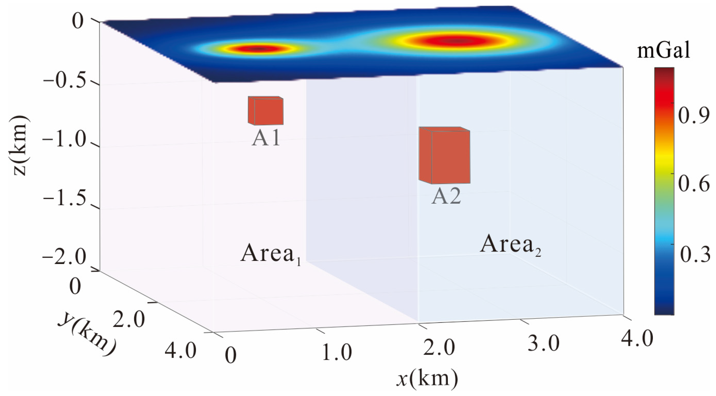
To verify the effectiveness of the ASW method, we set up two groups of model experiments. First, we established two prism models with different depths and sizes. Their parameters are given in

Table 1. Model parameters.

No.	Center Coordinates/m	Length/m	Width/m	Height/m	Density ρ (g/cm3)
A1	2000, 1050, 500	200	300	200	1.0
A2	2000, 2900, 900	400	400	400	1.0

. The model positions and gravity anomalies are shown in Figure 1. Both field sources had a density of 1 g/cm³. The underground was divided into 40 × 40 × 20 identical prismatic units. The grid step in the X and Y directions of the data was 100 m each. The subdivision and grid step size were consistent throughout the entire full-text model examination.

We applied the equivalent source method to forward the upward continuation anomaly and then used the upward continuation anomaly to compute DEXP imaging results. We determined the extent of the partition based on the location of the midpoints of the two maximum values of the imaging results, with x ≤ 2000 m as Area₁ and x > 2000 m as Area₂. We applied the ASW method to perform the inversion.

In Figure 2a, the depth of the field source can be seen as inconsistent, with deep field sources resulting in lower amplitudes. Thus, we partitioned the inversion space to make the distribution of the extreme values in the weighting function more reasonable. As shown in Figure 2b, after the partitioned calculation, the recovery capacity of the deep geological bodies was effectively improved. The partitioned weighting function can be seen to have better differentiation performance in the horizontal direction. The slices of $W_z{W}_{{\Omega }_i}$ with γ = 0.2 and $W_z{W}_{{\Omega }_i}$ with γ = 2 are shown in Figure 2c,d. At the same depth, $W_z{W}_{{\Omega }_i}$ function is characterized by high weights at the field source location and low weights at other locations. As γ increases, this feature will become more pronounced and a focus on the field source will appear. In order to visualize the weight distribution of the different functions more clearly, we extracted separately the change curves of the three weight functions at y = 2000 m, z = 900 m and y = 2000 m, z = 200 m, as shown in Figure 2e,f. We compared the variation of the three methods at different depths. At z = 900 m, the depth-weighting function is a fixed value of 17, as shown in Figure 2e. It does not reflect the geological bodies’ location information, which leads to the low resolution of inversion. As shown in Figure 2f, when γ = 0.2, the ASW function also increases in amplitude in the region where the geological bodies are located, which effectively reflects the distribution of field sources. Moreover, the amplitude is close to the depth-weighting function at the near-surface depth, which indicates that the ASW function can effectively counteract the attenuation effect of the kernel function. The calculated value range of W_Ω is 0~1. To ensure that the extreme value of the weighting function will still correspond to the center of the geological body, γ should be greater than zero. There was also a diffusion effect in the ratio DEXP results, so we squared the results.

The original anomaly was first inverted with a single depth-weighting function, and the slice at y = 2000 m is shown in Figure 3a. Then, the inversion was performed with the three weighting functions in Figure 2c–e, respectively. The final inversion results of the slice at y = 2000 m are shown in Figure 3b–d. As shown in Figure 3a, identifying deep rectangular bodies from these results using the depth-weighing function would be difficult. The inversion results from the use of the unpartitioned function in Figure 3b were improved to a certain extent to be more convergent after restraint. However, the amplitude recovery level for deep field sources still needed to be improved. The ASW function can effectively improve the ability to resolve deeper field sources. As shown in Figure 3c, the amplitude of the deep field source that was inverted with the ASW function was significantly increased and became closer to the actual value. As can be seen in Figure 3d, the recovery of the geological bodies with 2 as the value of γ was highly biased, with a clear demarcation of the entire space. The amplitude and range of the shallow geological body were very small, the correspondence with the center of the geological body was not accurate, and the ability to discriminate the bottom of the deep geological body was very low. We proved that the selection of too large of a value of γ can misdirect the iterative process and lead to lower precision of the inversion results. Therefore, if γ is excessively large, it amplifies the convergence at the center of the field source while reducing the response in other areas, which has a detrimental effect on the recovery of the field source morphology.

At the same time, we counted the difference between the inversion results of the two methods and the real situation, which was calculated as follows:

$$err=\left|\frac{\rho }{{\rho }_{\max }}-\frac{{\rho }_{real}}{{\rho }_{rea{l}_{\max }}}\right|$$

(17)

where $\rho$ is the computed inversion results, ${\rho }_{real}$ is the actual density distribution of the models, ${\rho }_{\max }$ corresponds to the maximum value of $\rho$, and ${\rho }_{rea{l}_{\max }}$ corresponds to the maximum value of ${\rho }_{real}$. The statistical results for the two areas are shown in Figure 3e–h. We compare the results of different inversion methods in terms of the proportion of errors. In Figure 3e, the proportion of errors more than 0.1 is 17.8% in Area₁ and 31.6% in Area₂. It was indicated that the results of inversion have large errors, especially in the area where the deeper geological body is located. As shown in Figure 3f, large deviations were significantly reduced using the unpartitioned space–location-weighting function, with which the proportion of errors that exceeded 0.1 was 2.5% in Area₁ and 16.4% in Area₂. The precision of the inversion results of the two geological bodies could be further improved with the ASW method. The majority of errors approached zero and the errors of the deeper geological body could be further reduced, approaching that of the shallower one. With this method, the proportion of errors that exceeded 0.1 was 1.9% in Area₁ and 9.4% in Area₂ as we can see in Figure 3g. At the same time, the distribution of the errors is decidedly not ideal in the case of γ = 2, which is shown in Figure 3h. The proportion of errors that exceeded 0.1 in this case was 7.6% in Area₁ and 18.4% in Area₂. Therefore, the value of γ cannot be more than 1. Under a multi-depth source distribution, the ASW function method exhibits space–location information, enabling it to better adapt to complex subsurface conditions in the realm of geophysics.

In order to make the simulated design anomalies resemble actual exploration data more closely, Gaussian noise with a signal-to-noise ratio (SNR) of 5 was added to the gravity data of the two models. The anomalies with noise are shown in Figure 4a, in which the value of γ is still 0.2. Similarly, the ASW function and the depth-weighting function were used to obtain slices of the final inversion results when y = 2000 m, as shown in Figure 4b–d, and the corresponding statistical results are shown in Figure 4e–g. Figure 4c reveals that in the case of the noise, the results after unpartitioned weighting calculation using space–location information were smoother. But the deep geological amplitude recovery was not ideal. As presented in Figure 4d, after the ASW method was used for guidance, the inversion results corresponded very well to the actual positions of the geological bodies, and the amplitude of the deeper geological bodies was increased. In comparison to Figure 4e–g, a similar situation to that of the two models without noise can be found. The proportion of errors that exceeded 0.1 of the inversion with the depth-weighting function was 24.3% in Area₁ and 16.5% in Area₂, as shown in Figure 4e. When compared to the depth-weighting method, the unpartitioned weighting method could decrease the proportion of errors with larger magnitudes. In Figure 4f, the proportion of Area₁ was 2.6% and that of Area₂ was 16.7%. However, as shown in Figure 4g, the precision could be further notably improved through the ASW method, with errors exceeding 0.1 at 1.8% in Area₁ and 9.2% in Area₂. Regardless of whether a geological body was deep or shallow, errors could be observed to be concentrated around zero. Thus, the ASW method has good noise resistance.

Finally, a single prism model was established to verify the applicability of the ASW function method. The center of the prism was at (2000, 2000, 600) m, the range was at (600, 600, 400) m, and the remaining density was 1 g/cm³. The gravity anomaly of one field source is shown in Figure 5a. The sampling interval was equal to the horizontal interval of the cells. In order to visually display the distribution of the weighting function, Figure 5d shows the central slice of the weight function results calculated with the ASW method. The normalized display is shown here for easy comparison of the strength of the weighting function. Obviously, the ASW function was more concentrated on the position where the field source was located, with the high values concentrated in the horizontal direction, and improvements were observed in the vertical direction.

Then, we performed a Fourier transformation of the gravity anomaly to obtain the power spectrum and the equivalent layer parameters. The gravity anomaly extended upward by 2000 m, and DEXP ratio imaging calculation was performed. We then used the ASW function method to establish the weighting function, in which $\gamma$ was 0.4. As shown in Figure 5c, the slice of the inversion results with the ASW method at y = 2000 m was also obtained. In order to compare the effects of the methods, the slices of both methods were processed with the same color scale. In a comparison of Figure 5c with Figure 5b, the inversion results with the ASW function are much closer to the real-field source distribution than the results with only the depth-weighting function, and the remaining density of the geological body can be better restored.

The results thereof are shown in Figure 5e,f. Using the convenient depth-weighting function would have given relatively large inversion result errors, but the errors when using the ASW function mostly concentrated around zero. The proportion of errors that exceeded 0.05 was 48% with the depth-weighting function and 8.1% with the ASW function. In terms of error statistics, the calculation results of the ASW function were more accurate. A modeling experiment demonstrated that the ASW method can still significantly improve the space resolution of inversion in the case of a single geological body.

4. Real Data Application

To verify the utility of the ASW method with actual data, we applied it to a region in Northwestern Shandong Province, China. This region has no bedrock outcrops, and Neogene and Quaternary strata are widely distributed there [27]. The area experiences regional tectonic movements during each geological history period, and the fracture structure is complex. Distribution is mainly in the NE, NNW, and SN directions, and the area has a locally developed fold structure and superior geological conditions for mineralization [28]. According to previous geological survey data, silica-type iron ores can be found in the study area. The main ore-controlling rocks are Ordovician carbonate [29]. Skarnization is an important alteration phenomenon that has mainly manifested as magnetite deposited above the high-density intrusive rock body [30] formed by the high-temperature hydrothermal contact interaction of the intermediate–basic intrusive rocks in this area [31]. Contact meta-somatic iron ore deposits are generally distributed near the edge of these intrusive rocks and the contact zone of limestone [29]. The location information and a geological map of the study area, as well as the logging data obtained according to a geological survey, are shown in Figure 6.

In order to obtain high precision density distribution of mineral resources in the region, a high-resolution airborne gravity survey with an average flying height of 86 m and a line distance of 200 m was designed and conducted. The measured gravity anomaly is shown in Figure 7a. Before the inversion, the measured gravity anomaly data were regridded using the minimum curvature method [32] to obtain the data with the grid size of 504 m × 576 m. After that, we denoised the gridded data, separated the potential field according to the power spectrum and extracted the region anomaly. Figure 7b shows the gravity anomaly obtained through data processing. The variation of the gravity anomalies in this region is well characterized by the distribution of faults. Three anomalies with large amplitudes are located in the survey area, in which three favorable zones for mineralization are initially determined. The iron ore deposits in the study area have high-density geophysical characteristics, so the ASW method was used to infer the location of these mineralization areas.

After Fourier transformation, we calculate the power spectrum curve of the gravity anomaly as shown in Figure 7c. The central depths of the equivalent layers were 849.4 m and 1506.6 m. Therefore, an equivalent layer was established based on the information above. The default number of layers was two, the thickness of the first layer was 465 m, the corresponding center depth was 850 m, the thickness of the second layer was 543 m, and the corresponding center depth was 1500 m. After the equivalent layer parameters were set, we obtained the gravity anomaly at 2000 m through upper prolongation and calculated W_Ωi, the results of which are shown in Figure 7c. Finally, based on the prior geological information, we set the maximum inversion depth to 2000 m, established the ASW function, and completed the inversion, with a γ of 0.25.

To clearly and intuitively show the depth of the top surface of the high-density bodies, slices of the inversion results at different depths are shown in Figure 8. The horizontal section at the depth of 860 m shows that the southernmost high-density body starts to show a weak response, so the top of a high-density body should be buried around this depth. In the 1220 m depth section, the other two bodies also show responses. In the deeper section, the three bodies showed stronger responses. We could identify the top surface burial depths of the three bodies from the inversion result: high-density body I is about 1307 m, body II is about 1190 m, and body III is about 834 m. The result corresponds well with the logging data. Because iron ore generally forms at the top interfaces of high-density bodies, ore bodies could possibly be produced in the horizontal ranges of their envelopes. The horizontal range of ore bodies based on this concept can be clearly recognized in Figure 8.

5. Conclusions

We proposed a high-precision density inversion method with an ASW function, which can improve the inversion resolution by introducing the location information to the weighting function. It can fully exploit the information contained in the data to adaptively design weighting functions and effectively constrain the inversion. A comparison of the inversion results of model tests proved that the precision of inversion results can be improved with the ASW method. Error statistics showed that accuracy for deeper sources can be improved by nearly 20% using the ASW method compared to inversion using the depth-weighting function, and the results also verified the stability of the ASW method against Gaussian noise. This method was applied to a mining area in Shandong. The ore body burial depth and spatial distribution characteristics of the geological mineralization bodies were estimated through inversion, which are verified by the logging results. Finally, we give the distribution of iron mines for future exploration.