
Fishery Resource Evaluation with Hydroacoustic and Remote Sensing in Yangjiang Coastal Waters in Summer


Abstract
:1. Introduction
2. Data and Methods
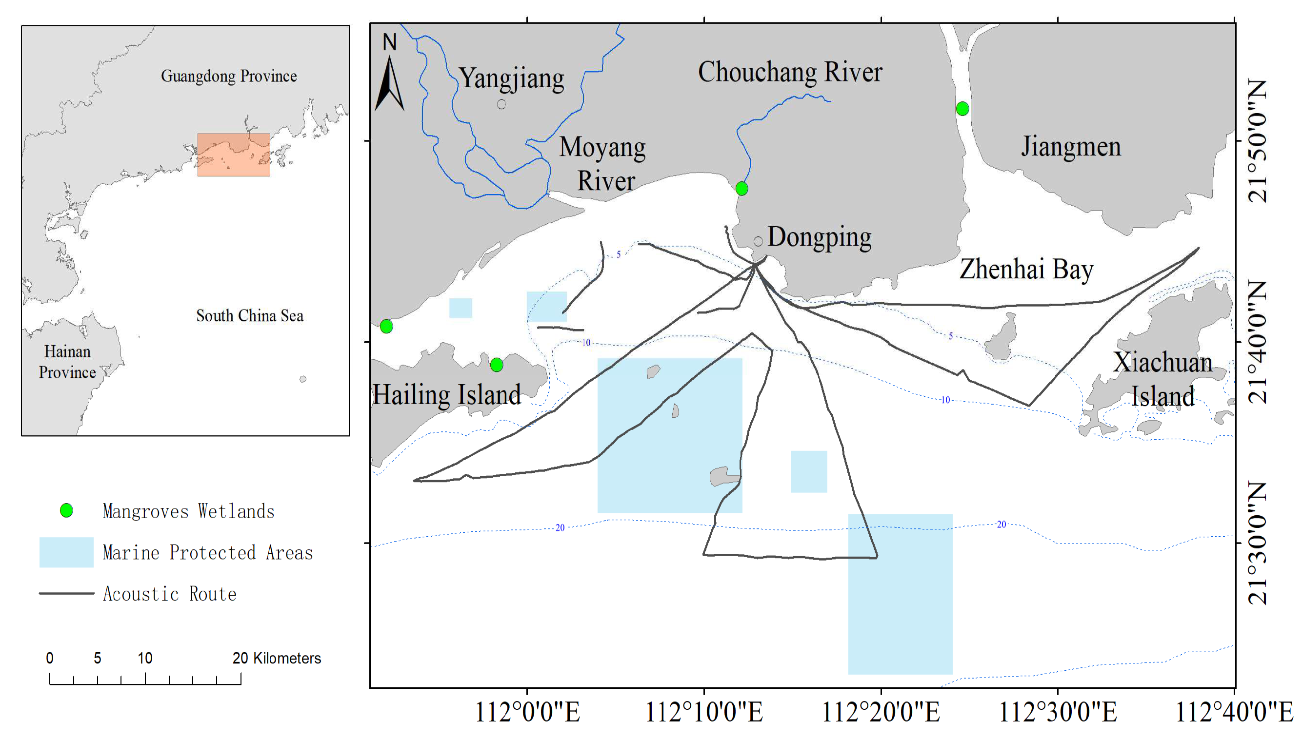
2.1. Study Area
2.2. Acoustic Data
2.3. Remote Sensing Data
2.4. Geostatistic Analysis
- (1)
- Normality distribution test was performed. If the conduction of normal distribution was not satisfied, logarithmic, reciprocals, square roots, inverse square roots or Box-Cox transformations were available;
- (2)
- Transformed data were modeled using the semi-variance function on the premise of isotropy. In general, there are 3 models: spherical, exponential, and Gaussian. The model is described by three parameters as follows [71]: (i) nugget, , Y-axis inter-cept of the model; (ii) sill, , asymptote of the model; (iii) range, a, spatial de-pendence is apparent when the distance greater than the parameter;
- (3)
- The parameters of residual sums of squares (RSS) and regression coefficient ( are all important indicators that can reflect a fitting degree of model. The most suitable model had the highest and smallest RSS. Then, kriging interpolation was per-formed based on the final model;
- (4)
- Verification of results. Cross-validation was adopted.
2.5. GAMs
3. Results
3.1. Size of Fish
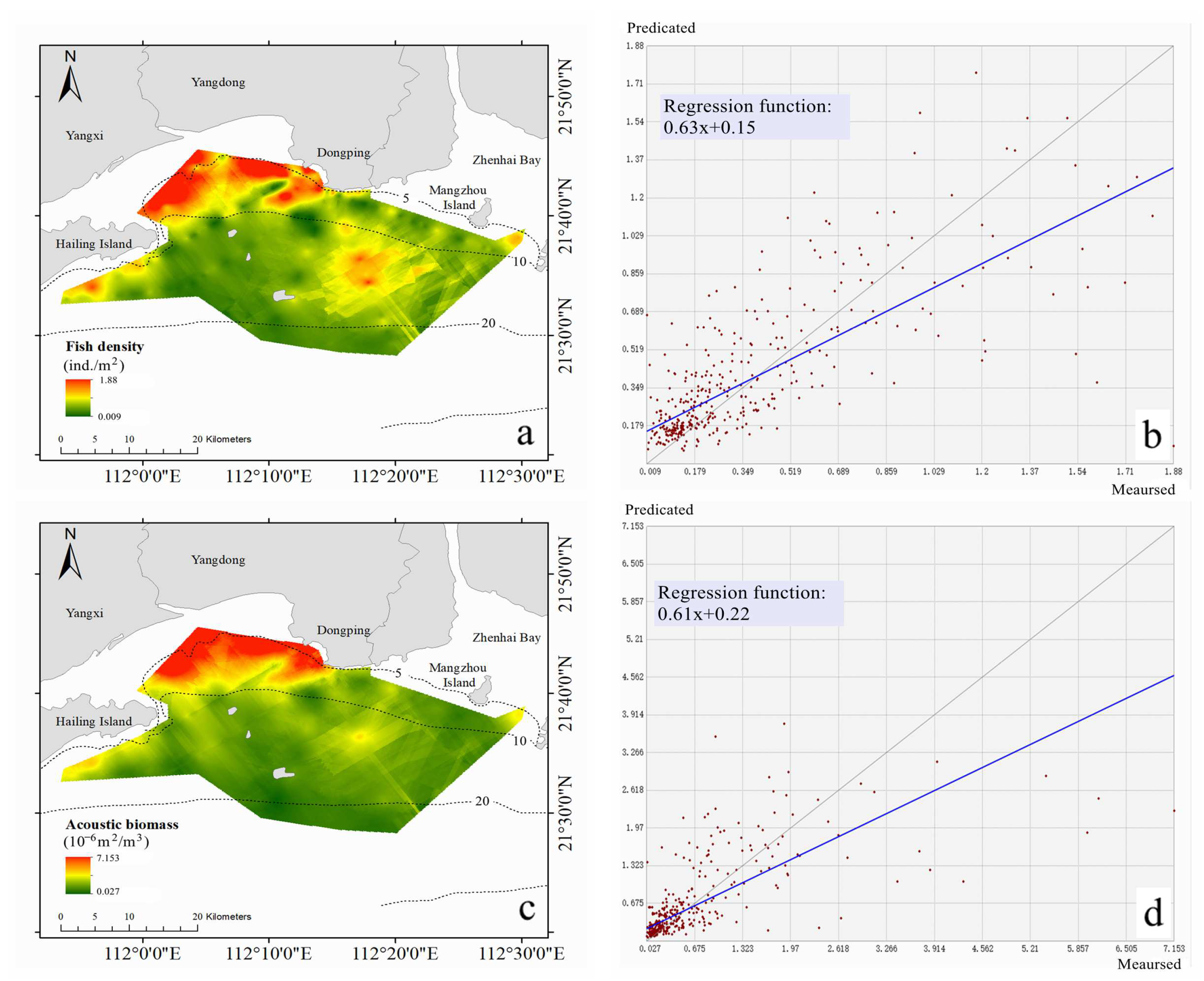
3.2. Distribution of Fish Density and Biomass Based on Geostatistic
3.3. Vertical Fish Density Distribution
3.4. Fish Density and Environmental Factors—GAM Model
4. Discussion
4.1. Size, Number and Distribution of Fish Resource
4.2. Relationship between Fish Density and Environmental Factors
4.3. Limitations and Prospects
5. Conclusions
- (1)
- Fish are mainly small individuals in Yangjiang coastal waters in summer;
- (2)
- The spatial distribution of fish density and acoustic biomass all had a characteristic of high nearshore and low offshore. Geostatistical analysis indicated that fish density and acoustic biomass had moderate spatial autocorrelation;
- (3)
- In vertical direction, fish usually inhabit waters of upper-middle depth in shallow water areas (<10 m), and in deeper water areas (>10 m), fish usually inhabit waters in the middle and bottom;
- (4)
- GAMs showed that SST, SSS, and longitude have a very significant correlation with fish density (p < 0.001), and chlorophyll has a significant correlation with fish density (p < 0.01).
Author Contributions
Funding
Data Availability Statement
Conflicts of Interest
References
- Hutchings, L.; Beckley, L.E.; Griffiths, M.H.; Roberts, M.J.; Sundby, S.; Lingen, C. Spawning on the edge: Spawning grounds and nursery areas around the southern African coastline. Mar. Freshw. Res. 2002, 53, 307–318. [Google Scholar] [CrossRef]
- Yu, J.; Chen, Z.; Xu, S. Land reclamation and its impact on fisheries resources in the Nansha wetland of Pearl River Estuary. J. Fish. Sci. China 2016, 23, 661–671. [Google Scholar]
- Ding, X.; Shan, X.; Chen, Y.; Li, M.; Li, J.; Jin, X. Variations in fish habitat fragmentation caused by marine reclamation activities in the Bohai coastal region, China. Ocean Coast. Manag. 2020, 184, 105038. [Google Scholar] [CrossRef]
- Yu, C.; Yu, C.; Zhang, F.; Ning, P. Fish species and quantity off southern Zhejiang East China Sea. Oceanol. Limnol. Sin. 2009, 40, 353–360. [Google Scholar]
- Chen, Z.; Xu, S.; Qiu, Y. A retrospective analysis of fishery resources and ecosystem evolution in the Beibu Gulf. In Proceedings of the Annual Academic Conference of Chinese Aquatic Society, Nanchang, China, 9–10 September 2017. [Google Scholar]
- Cheng, J.; Ding, F.; Li, S.; Yan, L.; Li, J.; Ling, Z. Changes of Fish Community Structure in the Coastal Zone of the Northern Part of East China Sea in Summer. J. Nat. Res. 2006, 21, 775–781. [Google Scholar]
- Haimovici, M.; Cardoso, L.G. Long-term changes in the fisheries in the Patos Lagoon estuary and adjacent coastal waters in Southern Brazil. Mar. Biol. Res. 2017, 13, 135–150. [Google Scholar] [CrossRef]
- Thykjaer, V.S.; Rodrigues, L.D.; Haimovici, M.; Cardoso, L.G. Long-term changes in fishery resources of an estuary in southwestern Atlantic according to local ecological knowledge. Fish. Manag. Ecol. 2020, 27, 185–199. [Google Scholar] [CrossRef]
- Holmer, M. Environmental issues of fish farming in offshore waters: Perspectives, concerns and research needs. Aquacult. Environ. Interact. 2010, 1, 57–70. [Google Scholar] [CrossRef] [Green Version]
- Brander, K.M. Global fish production and climate change. Proc. Natl. Acad. Sci. USA 2007, 104, 19709–19714. [Google Scholar] [CrossRef] [PubMed] [Green Version]
- Allison, E.H.; Perry, A.L.; Badjeck, M.C.; Adger, W.N.; Brown, K.; Conway, D.; Halls, A.S.; Pilling, G.M.; Reynolds, J.D.; Andrew, N.L. Vulnerability of national economies to the impacts of climate change on fisheries. Fish Fish. 2009, 10, 173–196. [Google Scholar] [CrossRef] [Green Version]
- Moose, P.H.; Throne, R.E.; Nelson, M.O. Hydroacoustics techniques for fishery resource assessment. Mar. Technol. Soc. J. 1971, 5, 35. [Google Scholar]
- Thorne, R.E.; Hedgepeth, J.B.; Campos, J. Hydroacoustic observations of fish abundance and behavior around and artifical reef in costarica. Bull. Mar. Sci. 1989, 44, 1058–1064. [Google Scholar]
- Stanley, D.R.; Wilson, C.A. Variation in the density and species composition of fishes associated with three petroleum platforms using dual beam hydroacoustics. Fish. Res. 2000, 47, 161–172. [Google Scholar] [CrossRef]
- Godlewska, M.; Colon, M.; Doroszczyk, L.; Długoszewski, B.; Verges, C.; Guillard, J. Hydroacoustic measurements at two frequencies: 70 and 120 kHz consequences for fish stock estimation. Fish. Res. 2009, 96, 11–16. [Google Scholar] [CrossRef]
- Lian, Y.; Huang, G.; Godlewska, M.; Cai, X.; Li, C.; Ye, S.; Liu, J.; Li, Z. Hydroacoustic estimates of fish biomass and spatial distributions in shallow lakes. Chin. J. Oceanol. Limnol. 2017, 36, 587–597. [Google Scholar] [CrossRef]
- Jack, P.E.; Mohsin, A.A.; Mohamed, A.; Mark, W.; Jamie, H.; John, T.; Brad, E.; Ibrahim, A.M.; Mohannadi, M.; Lewis, L.V. Hydroacoustics to examine fish association with shallow offshore habitats in the Arabian Gulf. Fish. Res. 2018, 199, 127–136. [Google Scholar]
- Guillard, J.; Vergès, C. The Repeatability of Fish Biomass and Size Distribution Estimates Obtained by Hydroacoustic Surveys Using Various Sampling Strategies and Statistical Analyses. Int. Rev. Hydrobiol. 2007, 92, 605–617. [Google Scholar] [CrossRef]
- Zhou, L.; Zeng, L.; Fu, D.; Xu, P.; Zeng, S.; Tang, Q.; Chen, Q.; Chen, L.; Li, G. Fish density increases from the upper to lower parts of the Pearl River Delta, China, and is influenced by tide, chlorophyll-a, water transparency, and water depth. Aquat. Ecol. 2016, 50, 59–74. [Google Scholar] [CrossRef]
- Li, B.; Chen, G.; Yu, J.; Wang, D.; Guo, Y.; Wang, Z. The acoustic survey of fisheries resources for various seasons in the mouth of Lingshui Bay of Hainan Island. J. Fish. China 2018, 42, 544–566. [Google Scholar]
- Coombs, R.F.; Cordue, P.L. Evolution of a stock assessment tool acoustic surveys of Spawning Hoki (Macruronus novaezelandiae) off the west coast of South Island, Newzealand, 1985–1991. N. Z. J. Mar. Freshw. Res. 1995, 29, 175–194. [Google Scholar] [CrossRef]
- Sala, A.; Fabi, G.; Manoukian, S. Vertical diel dynamic of fish assemblage associated with an artificial reef (Northern Adriatic Sea). Sci. Mar. 2007, 71, 355–364. [Google Scholar] [CrossRef]
- Zhang, J.; Chen, Z.; Chen, G.; Zhang, P.; Qiu, Y.; Yao, Z. Hydroacoustic studies on the commercially important squid Sthenoteuthis oualaniensis in the South China Sea. Fish. Res. 2015, 169, 45–51. [Google Scholar] [CrossRef]
- Zhang, J.; Chen, G.; Chen, Z.; Yu, J.; Fan, J.; Qiu, Y. Acoustic estimation of fishery resources in southern continental shelf of Nansha area. S. China Fish. Sci. 2015, 11, 1–10. [Google Scholar]
- Lucca, B.M.; Warren, J.D. Fishery-independent observations of Atlantic menhaden abundance in the coastal waters south of New York. Fish. Res. 2019, 218, 229–236. [Google Scholar] [CrossRef]
- Hamuna, B.; Pujiyatf, S.; Dimara, L.; Natief, N.M.N.; Alianto. Distribution and density of demersal fishes in Youtefa Bay, Papua, Indonesia: A study using hydroacoustic technology. India J. Fish. 2020, 67, 30–35. [Google Scholar] [CrossRef]
- Fotheringham, A.S. “The Problem of Spatial Autocorrelation” and Local Spatial Statistics. Geogr. Anal. 2009, 41, 398–403. [Google Scholar] [CrossRef]
- Liu, D.; Zhao, Q.; Guo, S.; Liu, P.; Xiong, L.; Yu, X.; Zou, H.; Zou, Y.; Wang, Z. Variability of spatial patterns of autocorrelation and heterogeneity embedded in precipitation. Hydrol. Res. 2019, 50, 215–230. [Google Scholar] [CrossRef] [Green Version]
- Wu, Z.; Zhang, C.; Xue, Y.; Ji, Y.; Ren, Y.; Xu, B. Spatial heterogeneity of demersal fish in the offshore waters of Shandong. Acta Oceanol. Sin. 2022, 44, 21–28. [Google Scholar]
- Matheron, G. Principles of Geostatistics. Econ. Geol. 1963, 58, 1246–1266. [Google Scholar] [CrossRef]
- Jorge, P.; Rubén, R. Acoustic-geostatistical assessment and habitat–abundance relations of small pelagic fish from the Colombian Caribbean. Fish. Res. 2003, 60, 309–319. [Google Scholar]
- Rubén, R.U.; Edwin, N. Biomass estimation from surveys with likelihood-based geostatistics. ICES J. Mar. Sci. 2007, 64, 1723–1734. [Google Scholar]
- Stratis, G.; Dimitra, K. Mapping abundance distribution of small pelagic species applying hydroacoustics and Co-Kriging techniques. Hydrobiologia 2008, 612, 155–169. [Google Scholar]
- Addis, P.; Secci, M.; Angioni, A.; Cau, A. Spatial distribution patterns and population structure of the sea urchin Paracentrotus lividus (Echinodermata: Echinoidea), in the coastal fishery of western Sardinia: A geostatistical analysis. Sci. Mar. 2012, 76, 733–740. [Google Scholar] [CrossRef] [Green Version]
- Thorson, J.T.; Shelton, A.O.; Ward, E.J.; Skaug, H.J. Geostatistical delta-generalized linear mixed models improve precision for estimated abundance indices for West Coast groundfishes. ICES J. Mar. Sci. 2015, 72, 1297–1310. [Google Scholar] [CrossRef]
- Castillo, R.; Aparco, L.L.C.; Grados, D.; Cornejo, R.; Guevara, R.; Csirke, A.J. Anchoveta (Engraulis ringens) Biomass in the Peruvian Marine Ecosystem Estimated by Various Hydroacoustic Methodologies during spring of 2019. J. Mar. Biol. Oceanogr. 2020, 9, 1000214. [Google Scholar]
- Galaiduk, R.; Radford, B.; Case, M.; Bond, T.; Taylor, M.; Cooper, T.; Smith, L.; McLean, D. Regional patterns in demersal fish assemblages among subsea pipelines and natural habitats across north-west Australia. Front. Mar. Sci. 2022, 9, 979987. [Google Scholar] [CrossRef]
- Fan, W.; Zhu, S.; Shen, J. An application of sattllite remote sensing-derived marine environmental factors to marine fisheries: A review. Mar. Sci. 2005, 29, 67–72. [Google Scholar]
- Strong, J.A.; Elliott, M. The value of remote sensing techniques in supporting effective extrapolation across multiple marine spatial scales. Mar. Pollut. Bull. 2017, 116, 405–419. [Google Scholar] [CrossRef] [PubMed]
- Zhang, X.; Li, Z.; Li, D.; He, Y. Marine Environment Distinctions and Change Law Based on eCongnition Remote Sensing Technology. J. Coast. Res. 2019, 94, 107–111. [Google Scholar] [CrossRef]
- Stenseth, N.C.; Mysterud, A.; Ottersen, G.; Hurrell, J.W.; Chan, K.S.; Lima, M. Ecological Effects of Climate Fluctuations. Science 2002, 297, 1292–1296. [Google Scholar] [CrossRef] [PubMed] [Green Version]
- DingsØr, G.E.; Ciannelli, L.; Chan, K.-S.; Ottersen, G.; Stenseth, N.C. Density dependence and density independence during the early life stages of four marine fish stocks. Ecology 2007, 88, 625–634. [Google Scholar] [CrossRef]
- Hastie, T.; Robert, T. Generalized Additive Models: Some Applications. J. Am. Stat. Assoc. 1985, 82, 371–386. [Google Scholar] [CrossRef]
- Gordon, S.; Emily, S.; Neal, W. Relating trends in walleye pollock (Theragra chalcogramma) abundance in the Bering Sea to environmental factors. Can. J. Fish. Aquat. Sci. 1995, 52, 369–380. [Google Scholar]
- Niu, M.; LI, X.; Xu, Y. Effects of spatiotemporal and environmental factors on the fishing ground of Trachurus murphyi in Southeast Pacific Ocean based on generalized additive model. Chin. J. Appl. Ecol. 2010, 21, 1049–1055. [Google Scholar]
- Tang, F.; Wu, Y.M.; Zhou, W.; Cui, X.; Fan, W.; Zhang, S. Study of marine environment and squid fishing fisheries in North Pacific Ocean based on remote sensing and GIS technology. In Proceeding of the 2nd International Conference on Energy and Environmental Protection (ICEEP 2013), Guilin, China, 20–21 April 2013. [Google Scholar]
- Setiawati, M.D.; Sambah, A.B.; Miura, F.; Tanaka, T.; As-syakur, A.R. Characterization of bigeye tuna habitat in the Southern Waters off Java-Bali using remote sensing data. Adv. Space Res. 2015, 55, 732–746. [Google Scholar] [CrossRef]
- Setiawati, M.D.; Tanaka, T. Utilization of Scatterplot Smoothers to Understand the Environmental Preference of Bigeye Tuna in the Southern Waters off Java-Bali: Satellite Remote Sensing Approach. Fishes 2017, 2, 2. [Google Scholar] [CrossRef]
- Wang, J.; Chen, X.; Chen, Y. Projecting distributions of Argentine shortfin squid (Illex argentinus) in the Southwest Atlantic using a complex integrated model. Acta Oceanol. Sin. 2018, 37, 31–37. [Google Scholar] [CrossRef]
- Wang, Y.; Yao, L.; Chen, P.; Yu, J.; Wu, Q. Environmental Influence on the Spatiotemporal Variability of Fishing Grounds in the Beibu Gulf, South China Sea. J. Mar. Sci. Eng. 2020, 8, 957. [Google Scholar] [CrossRef]
- Mammel, M.; Naimullah, M.; Vayghan, A.H.; Hsu, J.; Lee, M.; Wu, J.; Wang, Y.; Lan, K. Variability in the Spatiotemporal Distribution Patterns of Greater Amberjack in Response to Environmental Factors in the Taiwan Strait Using Remote Sensing Data. Remote Sens. 2022, 14, 2932. [Google Scholar] [CrossRef]
- Chen, Y.; Chen, Q. The present situation of the environmental protection of coastal waters in Yangjiang City and the countermesures for pollution prevention. Guangdong Chem. Ind. 2012, 39, 109. [Google Scholar]
- Yangdong District People Government. Planning of Aquaculture Tidal Flat in Yangdong District, Yangjiang (2018–2030); Yangdong District People Government: Yangjiang, China, 2019.
- Yangjiang Municipal Environmental Protection Bureau. Prevention and Control of Coastal Sea Pollution in Yangjiang City; Yangjiang Municipal Environmental Protection Bureau: Yangjiang, China, 2019.
- Thomsen, F.; Lüdemann, K.; Kafemann, R.; Piper, W. Effects of Offshore Wind Farm Noise on Marine Mammals and Fish; Cowrie Ltd.: Hamburg, Germany, 2006. [Google Scholar]
- Wilhelmsson, D.; Malm, T.; Ohman, M.C. The influence of offshore wind power on demersal fish. ICES J. Mar. Sci. 2006, 63, 775–784. [Google Scholar] [CrossRef] [Green Version]
- Berkel, J.V.; Burchard, H.; Christensen, A.; Mortensen, L.O.; Thomsen, F. The Effects of Offshore Wind Farms on Hydrodynamics and Implications for Fishes. Oceanography 2020, 33, 108–117. [Google Scholar] [CrossRef]
- Mai, G.; Chen, Z.; Wang, X.; Xiao, Y.; Li, C. Spatial pattern of fish taxonomic diversity along coastal waters in northern South China Sea. S. China Fish. Sci. 2022, 18, 38–47. [Google Scholar]
- Zhang, J.; Huang, Z. An investigation on fish eggs and larvae in sea area around planning Yangjiang neclear plant. J. Trop. Oceanogr. 2003, 22, 78–84. [Google Scholar]
- Jia, X.; Li, C.; Chen, Z.; Wang, X. Strategies for Managing Offshore Fishery Resources and Their Ecosystems in the Northern South China Sea; Ocean Press: Beijing, China, 2012. [Google Scholar]
- Wang, X.; Du, F.; Qiu, Y.; Li, C.; Li, D.; Jia, X. Variations of fish species diversity, faunal assemblage, and abundances in Daya Bay in 1980–2007. J. Appl. Ecol. 2010, 21, 2403–2410. [Google Scholar]
- Sun, P.; Shan, X.; Wu, Q.; Chen, Y.; Jin, X. Seasonal variations in fish community structure in the Laizhou Bay and the Yellow River Estuary. Acta Ecol. Sin. 2014, 34, 367–376. [Google Scholar]
- Liu, H.; Ye, Z.; Li, Z.; Hu, H.; Pang, Y.; Dou, S. The community structure of ichthyoplankton in the centural Yellow Sea in spring and summer. Acta Ecol. Sin. 2016, 36, 3775–3784. [Google Scholar]
- Xie, Z.; Sun, D.; Liu, Y.; Lin, L.; Wang, T.; Xiao, Y.; Li, C. Preliminary analysis of nekton composition and diversity in Jiangmen waters, China. S. China Fish. Sci. 2018, 14, 21–28. [Google Scholar]
- Yang, D.; Wu, G.; Sun, J. The investigation of pelagic eggs larvae and juveniles of fishes at the mouth of Changjiang River and adjacent areas. Oceanol. Limnol. Sin. 1990, 21, 346–355. [Google Scholar]
- Ding, Y.; Xian, W. Temporal and spatial structure of Ichthyoplankton assembleges in the Yangtze Estuary during autumn. Period. Ocean Univ. China 2011, 41, 67–74. [Google Scholar]
- Xiao, Y.; Wang, R.; Zheng, Y.; He, W. Species composition and abundance distribution of ichthyoplankton in the Pearl River Estuary. J. Trop. Oceanogr. 2013, 32, 80–87. [Google Scholar]
- Biosonics. User Guide: Visual Analyzer 4; BioSonics, Inc.: Seattle, WA, USA, 2002. [Google Scholar]
- Yin, X.; Yang, D.; Du, R. Fishery Resources Evaluation in Shantou Seas Based on Remote Sensing and Hydroacoustics. Fishes 2022, 7, 163. [Google Scholar] [CrossRef]
- Wang, Z.; Johnson, D.A.; Rong, Y.; Wang, K. Grazing effects on soil characteristics and vegetation of grassland in northern China. Solid Earth 2016, 7, 55–65. [Google Scholar] [CrossRef] [Green Version]
- Wang, A.; Wang, Q.; Li, J.; Yuan, G.; Albanese, S.; Petrik, A. Geo-statistical and multivariate analyses of potentially toxic elements’ distribution in the soil of Hainan Island (China): A comparison between the topsoil and subsoil at a regional scale. J. Geochem. Explor. 2019, 197, 48–59. [Google Scholar] [CrossRef]
- Feng, Y.; Yao, L.; Zhao, H.; Yu, J.; Lin, Z. Environmental Effects on the Spatiotemporal Variability of Fish Larvae in the Western Guangdong Waters, China. J. Mar. Sci. Eng. 2021, 9, 316. [Google Scholar] [CrossRef]
- Liu, S.; Liu, Y.; Alabia, I.D.; Tian, Y.; Ye, Z.; Yu, H.; Li, J.; Chen, J. Impact of Climate Change on Wintering Ground of Japanese Anchovy (Engraulis japonicus) Using Marine Geospatial Statistics. Front. Mar. Sci. 2020, 7, 604. [Google Scholar] [CrossRef]
- Love, R.H. Target strength of an individual fish at any aspect. J. Acoust. Soc. Am. 1977, 62, 1397–1403. [Google Scholar] [CrossRef]
- Fu, X.; Xu, Z.; Que, J.; Yan, T. Temporal-spatial Distribution Characíeristics of Fish Stocks in North-west Coastal Waters of Beibu Gulf. Fish. Sci. 2019, 38, 10–18. [Google Scholar]
- Guo, J.; Chen, Z.; Xu, Y.; Xu, S.; Li, C. Tempo-Spatial Distribution Characteristics of Fish Resources in Daya Bay. J. Ocean Univ. China 2018, 48, 47–55. [Google Scholar]
- Yan, L.; Tan, Y.; Yang, B.; Zhang, P.; Li, J.; Yang, L. Comparison on resources community of stow-net fishery before and after fishing off season in Huangmaohai Estuary. S. China Fish. Sci. 2016, 12, 1–8. [Google Scholar]
- Chen, X. Fishery Resources and Fisheries, 2nd ed.; Ocean Press: Beijing, China, 2014; pp. 152–167. [Google Scholar]
- Ma, Y.; Si, J. Study on monitoring of fish activity in the Yellow sea coastal water based on hydroacoustic technology. Fish. Modern. 2016, 43, 70–75. [Google Scholar]
- Wang, T.; Huang, H.H.; Zhang, P.; Zhang, S.F.; Wu, F.X.; Liu, Q.X.; Liao, X.L.; Xie, B. Acoustic survey of fisheries resources and spatial distribution in Guishan wind farm area. J. Fish. Sci. China 2020, 27, 1496–1504. [Google Scholar]
- Xu, Z. Comparison of fish density between the Minjiang Estuary and Xinghua Bay during spring and summer. J. Fish. China 2010, 34, 1395–1403. [Google Scholar]
- Zhang, J.; Luo, Y.; Li, Y.; Gao, T.; Lin, L. Temporal and Spatial Distribution of Species Composition and Quantity of Nekton in Dongshan Bay and Adjacent Areas. J. Ocean Univ. China 2013, 43, 44–51. [Google Scholar]
- Zhang, J.; Chen, P.; Fang, L.; Chen, G.; Li, X. Background acoustic estimation of fisheries resources in marine ranching area of Zhelin Bay-Nan’ao Island in the south China Sea. J. Fish. Sci. China 2015, 39, 1187–7798. [Google Scholar]
- Gu, Y. Study on Fish Community and Resources in Jiulong River Estuary, Fujian. Master’s Thesis, Jimei University, Xiamen, China, 2014. [Google Scholar]
- Zhang, G.; Yang, C.; Sun, D.; Liu, Y.; Shan, B.; Zhao, Y.; Zhou, W. Seasonal variation of fish community in north central region of Beibu Gulf. J. South Agric. 2021, 52, 2861–2871. [Google Scholar]
- Hu, C.; Zhang, Y.; Li, D.; Zhu, W.; Jiang, R.; Li, P.; Wang, Y.; Zhou, Y.; Zhang, H. Study on fish resources and community diversity during spring and summer in the coastal spawning ground of Zhejiang Proviance, China. Acta Hydrobiol. Sin. 2018, 42, 984–995. [Google Scholar]
- Cai, M.; Xu, Z. Species composition and density of fishes in the Sanmen Bay. J. Sci. Fish. Univ. 2009, 18, 198–205. [Google Scholar]
- Chen, W.; Ye, S.; Qin, S.; Fan, Q.; Chen, S.; Ni, Y.; Peng, X. Assessment of fish community structure and redundancy analysis of dominant species in the Oujiang River estuary. J. Fish. Sci. China 2021, 28, 1536–1547. [Google Scholar]
- Liu, Y.; Ye, S.; Ma, C.; Zhuang, Z.; Xu, C.; Shen, C.; Cai, J.; Xie, S. Seasonal variations in species and the quantity of nekton in Sansha Bay. Fujian Mar. Sci. 2022, 46, 86–94. [Google Scholar]
- Donelson, J.M.; Munday, P.L.; Mccormick, M.I.; Nilsson, G.E. Acclimation to predicted ocean warming through developmental plasticity in a tropical reef fish. Glob. Chang. Biol. 2011, 17, 1712–1719. [Google Scholar] [CrossRef]
- Sims, D.W.; Wearmouth, V.J.; Genner, M.J.; Southward, A.J.; Hawkins, S.J. Low-temperature-driven early spawning migration of a temperate marine fish. J. Anim. Ecol. 2004, 73, 333–341. [Google Scholar] [CrossRef]
- Fu, X. Distribution of Fish Populations and Structure of Fish Communities in the Coastal Waters of Northwest Beibu Gulfand Their Influential Factors. Master’s Thesis, Shanghai Ocean University, Shanghai, China, 2018. [Google Scholar]
- Love, J.W.; May, E.B. Relationships between fish assemblage structure and selected environmental factors in Maryland’s coastal bays. Northeast. Nat. 2007, 14, 251–268. [Google Scholar] [CrossRef]
- Yu, N.; Yu, C.; Xu, Y.; Chen, L.; Xu, H.; Wang, H.; Zhang, P.; Liu, K. The relationship between distribution of fish abundance and environmental factors in the outer waters of the Zhoushan Islands. Acta Oceanolog. Sin. 2020, 42, 80–91. [Google Scholar]
- Eppley, R.W.; Stewart, E.; Abbott, M.R.; Heyman, U. Estimating Ocean primary production from satellite chlorophyll. Introduction to regional differences and statistics for the Southern California Bight. J. Plankton Res. 1985, 7, 57–70. [Google Scholar] [CrossRef]
- Maryann, M.; Joseph, J.C.J. Osmoregulation in juvenile and adult white sturgeon, Acipenser transmontanus. Environ. Biol. Fish. 1985, 14, 23–30. [Google Scholar]
- Wan, J.; Zeng, D.; Bian, X.; Ni, X. Species composition and abundance distribution pattern of ichthyoplankton and their relationship with environmental factors in the East China Sea ecosystem. J. Fish. China 2014, 38, 1375–1398. [Google Scholar]
- Zou, M.; Chen, Y.; Song, X.; Li, S.; Zhong, J. Distribution and drift trend of Collichthys lucidus larvae and juveniles in the coastal waters of the southern Yellow Sea. J. Fish. China 2021, 46, 557–568. [Google Scholar]
- Niu, M.; Zuo, T.; Wang, J.; Chen, R.; Zhang, J. Egg and larval distribution of Liza haematochezia and their relationship with environmental factors in the coastal waters of the Yellow River Estuary. J. Fish. Sci. China 2022, 29, 377–387. [Google Scholar]
- Kim, J.Y.; Kim, J.I.; Choi, S.G.; Chun, Y.Y.; Choi, I. Factors Affecting the Wintering Habitat of Major Fishery Resources in Southwestern Korean Waters. Ocean Sci. J. 2007, 42, 41–48. [Google Scholar] [CrossRef]
- Kim, J.Y.; Lee, S.K.; Kim, S.S.; Choi, M.S. Environmental factors affecting anchovy reproductive potential in the southern coastal waters of Korea. Anim. Cells Syst. 2013, 17, 133–140. [Google Scholar] [CrossRef] [Green Version]
- Lappalainen, A.; Shurukhin, A.; Alekseev, G.; Rinne, J. Coastal fish communities along the northern coast of the Gulf of Finland, Baltic Sea: Responses to salinity and eutrophication. Int. Rev. Hydrobiol. 2000, 85, 687–696. [Google Scholar] [CrossRef]
- Rodriguez-Climent, S.; Caiola, N.; Ibanez, C. Salinity as the main factor structuring small-bodied fish assemblages in hydrologically altered Mediterranean coastal lagoons. Sci. Mar. 2013, 77, 37–45. [Google Scholar]
- Morin, B.; Hudon, C.; Whoriskey, F.G. Environmental- influences on seasonal distribution of coastal and estuarine fish assemblages at Wemindji, Eastern James Bay. Environ. Biol. Fishes 1992, 35, 219–229. [Google Scholar] [CrossRef]
- Zhang, Y.; Xian, W.; Li, W. Fish assemblage structure in adjacent sea of Changjiang estuary in spring of 2004 and 2007 and its association with environmental factors. Period. Ocean Univ. China 2013, 43, 67–74. [Google Scholar]
- Axenrot, T.; Didrikas, T.; Danielsson, C.; Hansson, S. Diel patterns in pelagic fish behaviour and distribution observed from a stationary, bottom-mounted, and upward-facing transducer. ICES J. Mar. Sci. 2004, 61, 2004. [Google Scholar] [CrossRef]
- Fréon, P.; Gerlotto, F.; Soria, M. Diel variability of school structure with special reference to transition periods. ICES J. Mar. Sci. 1996, 53, 459–464. [Google Scholar] [CrossRef] [Green Version]
- Gauthier, S.; Rose, G.A. Acoustic observation of diel vertical migration and shoaling behaviour in Atlantic redfishes. J. Fish Biol. 2005, 61, 1135–1153. [Google Scholar] [CrossRef]
- Totland, A.; Johansen, G.O.; Godø, O.R.; Ona, E.; Torkelsen, T. Quantifying and reducing the surface blind zone and the seabed dead zone using new technology. ICES J. Mar. Sci. 2009, 66, 1370–1376. [Google Scholar] [CrossRef] [Green Version]
- Robertis, A.D.; Handegard, N.O. Fish avoidance of research vessels and the efficacy of noise-reduced vessels: A review. ICES J. Mar. Sci. 2013, 70, 34–45. [Google Scholar] [CrossRef]
- Knudsena, F.R.; Sægrov, H. Benefits from horizontal beaming during acoustic survey: Application to three Norwegian lakes. Fish. Res. 2002, 56, 205–211. [Google Scholar] [CrossRef]
- Blaber, S.J.M.; Blaber, T.G. Factors affecting the distribution of juvenile estuarine and inshore fish. J. Fish Biol. 1980, 17, 143–162. [Google Scholar] [CrossRef]
- Rakocinski, C.F.; Baltz, D.M.; Fleeger, J.W. Correspondence between environmental gradients and the community structure in Mississippi Sound as revealed by canonical correspondence analysis. Mar. Ecol. Prog. Ser. 1992, 80, 135–148. [Google Scholar] [CrossRef]
- Fraser, T.H. Abundance, seasonality, community indices, trends and relationships with physicochemical factors of trawled fish in upper Charlotte Harbor, Florida. Bull. Mar. Sci. 1997, 60, 739–763. [Google Scholar]
- Albaret, J.J.; Simier, M.; Darboe, F.S.; Ecoutin, J.M.; Raffray, J.; Morais, L.T. Fish diversity and distribution in the Gambia Estuary, West Africa, in relation to environmental variables. Aquat. Living Resour. 2004, 17, 35–46. [Google Scholar] [CrossRef]
- Liu, Z.; Yang, L.; Yan, L.; Yuan, X.; Cheng, J. Fish assemblages and environmental interpretation in the northern Taiwan Strait and its adjacent waters in summer. J. Fish. Sci. China 2016, 23, 1399–1416. [Google Scholar]
- Thorman, S. Physical factors affecting the abundance and species richness of fishes in the shallow waters of the southern Bothnian Sea (Sweden). Estuar. Coast. Shelf Sci. 1986, 22, 357–369. [Google Scholar] [CrossRef]
- Smith, C.L.; Hill, A.E.; Foreman, M.G.; Peña, M.A. Horizontal transport of marine organisms resulting from interactions between diel vertical migration and tidal currents off the west coast of Vancouver Island. Can. J. Fish. Aquat. Sci. 2001, 58, 736–748. [Google Scholar] [CrossRef]
- Rodríguez, J.M.; Hernández-León, S.; Barton, E.D. Vertical distribution of fish larvae in the Canaries-African coastal transition zone in summer. Mar. Biol. 2006, 149, 885–897. [Google Scholar] [CrossRef] [Green Version]
- Wang, Z.; DiMarco, S.F.; Ingle, S.; Belabbassi, L.; Al-Kharusi, L.H. Seasonal and annual variability of vertically migrating scattering layers in the northern Arabian Sea. Deep Sea Res. Part I Oceanogr. Res. Pap. 2014, 90, 152–165. [Google Scholar] [CrossRef]


| Variables | Units | Mean | Range | Description |
|---|---|---|---|---|
| SST | °C | 29.65 ± 0.27 | 29.25–30.13 | Sea surface temperature |
| Chlorophyll-a | mg/m3 | 4.21 ± 2.20 | 0.37–10.53 | Chlorophyll concentration |
| Salinity | psu | 33.08 ± 0.45 | 31.90–33.51 | Sea surface salinity |
| SSTA | °C | 1.30 ± 0.25 | 0.89–1.72 | Sea surface temperature anomaly |
| Depth | m | 13.11 ± 4.82 | 5.86–22.3 | Water depth |
| Variables | VIF |
|---|---|
| Lon | 1.051 |
| SST | 2.046 |
| Chla | 3.072 |
| SSS | 1.864 |
| Model | AIC |
|---|---|
| log(FPUA + 1) ~ s(SST) | −50.442 |
| log(FPUA + 1) ~ s(SST) + s(Chla) | −81.159 |
| log(FPUA + 1) ~ s(SST) + s(Chla) + s(SSS) | −89.251 |
| log(FPUA + 1) ~ s(SST) + s(Chla) + s(SSS) + s(Lon) | −104.401 |
| Variable | Density | Biomass | ||||
|---|---|---|---|---|---|---|
| Model | Exponential | Spherical | Gaussian | Exponential | Spherical | Gaussian |
| Nugget (C0) | 0.0128 | 0.0048 | 0.0125 | 0.1213 | 0.0119 | 0.0301 |
| Sill (C0 + C) | 0.0739 | 0.0729 | 0.0729 | 0.2436 | 0.1798 | 0.1802 |
| Range (A)/m | 5040 | 2820 | 2372.91 | 74,250 | 19,600 | 14,849.23 |
| RSS | 2.422 × 10⁻⁴ | 3.423 × 10⁻⁴ | 3.392 × 10⁻⁴ | 3.67 × 10⁻³ | 9.037 × 10⁻³ | 8.994 × 10⁻³ |
| R2 | 0.743 | 0.632 | 0.635 | 0.717 | 0.302 | 0.306 |
| Nugget coefficient (C0/(C0 + C) | 0.273 | 0.066 | 0.171 | 0.498 | 0.066 | 0.167 |
| Variables | Edf | F | Accumulation of Deviance Explanation/% | Deviance Explanation of Each Factor/% | p |
|---|---|---|---|---|---|
| SST | 2.266 | 24.499 | 35.3 | 35.3 | 9.23 × 10⁻¹¹ *** |
| Chla | 1.000 | 7.328 | 47.1 | 11.8 | 0.0077 ** |
| SSS | 6.284 | 5.444 | 52.7 | 5.6 | 1.34 × 10⁻⁵ *** |
| Longitude | 2.466 | 5.795 | 59.2 | 6.5 | 7.68 × 10⁻⁴ *** |
| Region | Time | Fish Density (105 ind./km2) | Method | Source |
|---|---|---|---|---|
| Xinghua Bay | September 2008 | 0.582 | Trawl | [81] |
| Min River Estuary | September 2008 | 1.588 | Trawl | [81] |
| Dongshan Bay | August 2010 | 0.106 | Trawl | [82] |
| Zhelin bay | August 2011 | 0.649 | Hydroacoustic | [83] |
| Jiulong River Estuary | August 2013 | 0.571 | Set and gill net | [84] |
| Qinzhou coastal waters | August 2016 | 1.248 | Trawl | [85] |
| Zhejiang coastal waters | July 2015 | 2.055 | Trawl | [86] |
| Lingshui Bay | August 2015 | 1.11 | Hydroacoustic | [20] |
| Daya Bay | August 2015 | 1.066 | Trawl | [76] |
| Sanmen Bay | June 2018 | 0.2888 | Trawl | [87] |
| Oujiang estuary | August 2018 | 3.39 | Trawl | [88] |
| Sansha Bay | July 2019 | 0.121 | Set-net | [89] |
| Yangjiang coastal waters | July 2021 | 3.75 | Hydroacoustic | This study |
Disclaimer/Publisher’s Note: The statements, opinions and data contained in all publications are solely those of the individual author(s) and contributor(s) and not of MDPI and/or the editor(s). MDPI and/or the editor(s) disclaim responsibility for any injury to people or property resulting from any ideas, methods, instructions or products referred to in the content. |
© 2023 by the authors. Licensee MDPI, Basel, Switzerland. This article is an open access article distributed under the terms and conditions of the Creative Commons Attribution (CC BY) license (https://creativecommons.org/licenses/by/4.0/).
Share and Cite
Yin, X.; Yang, D.; Zhao, L.; Zhong, R.; Du, R. Fishery Resource Evaluation with Hydroacoustic and Remote Sensing in Yangjiang Coastal Waters in Summer. Remote Sens. 2023, 15, 543. https://doi.org/10.3390/rs15030543
Yin X, Yang D, Zhao L, Zhong R, Du R. Fishery Resource Evaluation with Hydroacoustic and Remote Sensing in Yangjiang Coastal Waters in Summer. Remote Sensing. 2023; 15(3):543. https://doi.org/10.3390/rs15030543
Chicago/Turabian StyleYin, Xiaoqing, Dingtian Yang, Linhong Zhao, Rong Zhong, and Ranran Du. 2023. "Fishery Resource Evaluation with Hydroacoustic and Remote Sensing in Yangjiang Coastal Waters in Summer" Remote Sensing 15, no. 3: 543. https://doi.org/10.3390/rs15030543