Multi-Source Interactive Stair Attention for Remote Sensing Image Captioning

Abstract

The aim of remote sensing image captioning (RSIC) is to describe a given remote sensing image (RSI) using coherent sentences. Most existing attention-based methods model the coherence through an LSTM-based decoder, which dynamically infers a word vector from preceding sentences. However, these methods are indirectly guided through the confusion of attentive regions, as (1) the weighted average in the attention mechanism distracts the word vector from capturing pertinent visual regions and (2) there are few constraints or rewards for learning long-range transitions. In this paper, we propose a multi-source interactive stair attention mechanism that separately models the semantics of preceding sentences and visual regions of interest. Specifically, the multi-source interaction takes previous semantic vectors as queries and applies an attention mechanism on regional features to acquire the next word vector, which reduces immediate hesitation by considering linguistics. The stair attention divides the attentive weights into three levels—that is, the core region, the surrounding region, and other regions—and all regions in the search scope are focused on differently. Then, a CIDEr-based reward reinforcement learning is devised, in order to enhance the quality of the generated sentences. Comprehensive experiments on widely used benchmarks (i.e., the Sydney-Captions, UCM-Captions, and RSICD data sets) demonstrate the superiority of the proposed model over state-of-the-art models, in terms of its coherence, while maintaining high accuracy.

1. Introduction

Transforming vision into language has become a hot topic in the field of artificial intelligence in recent years. As a joint task of image understanding and language generation, image captioning [1,2,3,4] has attracted the attention of more and more researchers. Specifically, the task of image captioning generates comprehensive and appropriate natural language, according to the content of the image. It is necessary to deeply study and understand the object, scene, and their relationship in the image for appropriate sentence generation. Due to the novelty and creativity of this task, image captioning has various application prospects, including human–computer interaction, blind assistant, battlefield environment analysis, and so on.

With the rapid development of remote sensing technologies, the quantity and quality of remote sensing images (RSIs) have achieved great progress. Through these RSIs, we can observe the earth from an unprecedented perspective. Indeed, there are many differences between RSIs and natural images. First, RSIs usually contain large scale differences, causing the scene range and object size of RSIs to differ from that of natural images. Furthermore, the modality of objects in RSIs is also very different from that in a natural image with overhead imaging. The rich information contained in an RSI can be further mined by introducing the task of image captioning into the RSI field, and the applications of the RSI can be further broadened. Many tasks, such as scene classification [5,6,7], object detection [8,9], and semantic segmentation [10,11], focus on obtaining image category labels or object locations and recognition. Remote sensing image captioning (RSIC) can extract more ground feature information, attributes, and relationships in RSIs, in the form of natural language to facilitate human understanding.

1.1. Motivation and Overview

In order to determine the corresponding relationship between the generated words and the image region, spatial attention mechanisms have been proposed and widely used in previous studies [12,13]. Through the use of spatial attention mechanisms, such as hard attention or soft attention [2], different regions of the image feature map can be given different weights, such that the decoder can focus on the image regions related to the words being generated. However, this correspondence leads to more attention being paid to the location of the object, without full utilization of the semantic information of the object and the text information of the generated sentence. In a convolutional neural network (CNN), each convolution kernel encodes a pattern: a shallow convolution kernel encodes low-level visual information, such as colors, edges, and corners, while a high-level convolution kernel encodes high-level semantic information, such as the category of an object [14]. Each channel of the high-level feature map represents a semantic attribute [4]. These semantic attributes are not only important visual information in the image, but also important components in the language description, which can help the model to understand the object and its attributes more accurately. In addition, part of the generated sentence also contains an understanding of the image. According to the generated words, some prepositions and function words can be generated. On the other hand, most existing methods lack direct supervision to guide the long-range sentence transition. The widely used maximum likelihood estimation (i.e., cross-entropy) promotes accuracy in word prediction, but provides little feedback for sentence generation in a given context. Reinforcement Learning (RL) has achieved great success in natural image captioning (NIC) by addressing the gap between training loss and evaluation metrics. Vaswani et al. [15] have presented an RL-based self-critical sequence training (SCST) method, which improves the performance of image captioning considerably. Through the effective combination of the above approaches, we can enhance the understanding of the image content, thus obtaining more accurate sentences. Inspired by the physiological structure of human retinal imaging [16], we re-think the construction of spatial attention weighting. Being able to distinguish the color and detail of objects better, the cone cells are mainly distributed near the fovea, and less around the retina. This distribution pattern of the cone cells has an important impact on human vision. In this line, a new spatial attention mechanism is constructed in this paper.

Motivated by the above-mentioned reasons, we propose a multi-source interactive stair attention (MSISAM) network. The proposed method mainly includes two serial attention networks. One is a multi-source interactive attention (MSIAM) network. Different from the spatial attention mechanism, focusing on the corresponding relationships between words and image regions, it introduces the rich semantic information contained in the channel dimension and the context information in the generated caption fragments. By using a variety of information, the MSIAM network can selectively pay attention to the feature maps output by CNNs. The other is the stair attention network, which is followed by the MSIAM network, and in which the attentive weights are stair-like, according to the degree of attention. Specifically, the calculated weights are shifted to the area of interest in order to reduce the weight of the non-attention area. In addition, we devise a CIDEr-based reward for RL-based training. This enhances the quality of long-range transitions and trains the model more stably, improving the diversity of the generated sentences.

1.2. Contributions

The core contributions of this paper can be summarized as follows:

(1) A novel multi-source interactive attention network is proposed, in order to explore the effect of semantic attribute information of RSIs and the context information of generated words to obtain complete sentences. This attention network not only focuses on the relationship between the image region and the generated words, but also improves the utilization of image semantics and sentence fragments. A variety of information works together to allocate attention weights, in terms of space and channel, to build a semantic communication bridge between image and text.

(2) A cone cell heuristic stair attention network is designed to redistribute the existing attention weights. The stair attention network highlights the most concerned image area, further weakens the weights far away from the concerned area, and constructs a closer mapping relationship between the image and text.

(3) We further adopt a CIDEr-based reward to alleviate long-range transitions in the process of sentence generation, which takes effect during RL training. The experimental results show that our model is effective for the RSIC task.

1.3. Organization

The remainder of this paper is organized as follows. In Section 2, some previous works are briefly introduced. Section 3 presents our approach to the RSIC task. To validate the proposed method, the experimental results are provided in Section 4. Finally, Section 5 briefly concludes the paper.

2. Related Work

2.1. Natural Image Captioning

Many ideas and methods of the RSIC task come from the NIC task; therefore, it is necessary to consider the research progress and research status in the NIC field. With the publication of high-quality data sets, such as COCO, flickr8k, and flickr30k, the NIC task also uses deep neural networks to achieve end-to-end sentence generation. Such end-to-end implementations are commonly based on the encoder–decoder framework, which is the most widely used frameworks in this field. These methods follow the same paradigm: a CNN is used as an encoder to extract image features, and a recurrent neural network (RNN) or long short-term memory (LSTM) network [17] is used as a decoder to generate a description statement.

Mao et al. [18] have proposed a multi-modal recurrent neural network (M-RNN) which uses the encoder–decoder architecture, where the interaction of the CNN and RNN occurs in the multi-modal layer to describe RSIs. Compared with RNN, LSTM solves the problem of gradient vanishing while preserving the correlation of long-term sequences. Vinyals et al. [1] have proposed a natural image description generator (NIC) model in which the RNN was replaced by an LSTM, making the model more convenient for long sentence processing. As the NIC model uses the image features generated by the encoder at the initial time when the decoder generates words, the performance of the model is restricted. To solve this problem, Xu et al. [2] have first introduced the attention mechanism in the encoder–decoder framework, including hard and soft attention mechanisms, which can help the model pay attention to different image regions at different times, then generate different image feature vectors to guide the generation of words. Since then, many methods based on attention mechanisms have been proposed.

Lu et al. [19] have used an adaptive attention mechanism—the “visual sentinel”—which helped the model to adaptively determine whether to focus on image features or text features. When the research on spatial attention mechanisms was in full swing, Chen et al. [20] proposed the SCA-CNN model, using both a spatial attention mechanism and a channel attention mechanism in order to make full use of image channel information, which improved the model’s perception and selection ability of semantic information in the channel dimension. Anderson et al. [21] have defined the attention on image features extracted from CNNs as top-down attention. Concretely, Faster R-CNN [22] was used to obtain bottom-up attention features, which were combined with top-down attention features for better performance. Research has shown that bottom-up attention also has an important impact on human vision.

In addition, the use of an attention mechanism on advanced semantic information can also improve the ability of NIC models to describe key visual content. Wu et al. [23] have studied the role of explicit high-level semantic concepts in the image content description. First, the visual attributes in the image are extracted using a multi-label classification network, following which they are introduced into the decoder to obtain better results. As advanced image features, the importance of semantics or attributes in images has also been discussed in [24,25,26]. The high-level attributes [27] have been directly employed for NIC. The central spirit of this scheme aimed to strengthen the vision–language interaction using a soft-switch pointer. Tian et al. [28] have proposed a controllable framework that can generate captions grounded on related semantics and re-ranking sentences, which are sorted by a sorting network. Zhang et al. [29] have proposed a transformer-based NIC model based on the knowledge graph. The transformer applied multi-head attention to explore the relation between the object features and corresponding semantic information. Rennie et al. [30] have considered the problem that the evaluation metrics could not correspond to the loss function in this task. Thus, an SCST RL-based method [15] has been proposed to deal with the above problem.

2.2. Remote Sensing Image Captioning

Research on RSIC started later than that of NIC. However, some achievements have emerged by combining the characteristics of RSIs with the development of NIC. Shi et al. [31] have proposed a template-based RSIC model. The full convolution network (FCN) first obtains the object labels, and then a sentence template matches semantic information to generate corresponding descriptions. Wang et al. [32] have proposed a retrieval-based RSIC method, which selects the sentence closest to the input image in the representation space as its description. The encoder–decoder structure is also popular in the field of RSIC. Qu et al. [33] have explored the performance of a CNN + LSTM structure to generate corresponding captions for RSIs, and disclosed results on two RSIC data sets (i.e., UCM-captions and Sydney-captions). Many studies on attention-based RSIC models have recently been performed; for example, Lu et al. [3] have explored the performance of an attention-based encoder–decoder model, and disclosed results on the RSICD data set. The RSICD further promotes the development of the RSIC task. The scene-level attention can produce scene information for predicting the probability of each word vector. Li et al. [34] have proposed a multi-level attention (MLA) including attention on image spatial domain, attention on different texts, and attention for the interaction between vision and text, which further enriched the connotation of attention mechanisms in RSIC task. Some proposed RSIC models have aimed to achieve better representations of the input RSI, and can alleviate the scale diversity problem, to some extent. For example, Ahmed et al. [35] have introduced a multi-scale multi-interaction network for interacting multi-scale features with a self-attention mechanism. The recurrent attention and semantic gate (RASG) [36] utilizes dilated convolution filters with different dilation rates to learn multi-scale features for numerous objects in RSIs. In the decoding phase, the multi-scale features are decoded by the RASG, focusing on relevant semantic information. Zhao et al. [37] have produced segmentation vectors in advance, such as hierarchical regions, in which the region vectors are combined with the spatial attention to construct the sentence-level decoder. Unlike multi-scale feature fusion, meta learning has been introduced by Yang et al. [38], where the encoder inherited excellent performance by averaging several discrete task embeddings clustered from other image libraries (i.e., natural images and RSIs for classification). Most previous approaches have ignored the gap between linguistic consistency and image content transition. Zhang et al. [4] have further generated a word-vector using an attribute-based attention to guide the captioning process. The attribute features were trained to highlight words that occurred in RSI content. Following this work, the label-attention mechanism (LAM) [39] controlled the attention mechanism with scene labels obtained by a pre-trained image classification network. Lu et al. [40] have followed the branch of sound topic transition for the input RSI; but, differently, the semantics were separated from sound information to guide the attention mechanism. For the problem of over-fitting in RS caption generation caused by CE loss, Li et al. [41] have improved the optimization strategy using a designed truncated cross-entropy loss. Similarly, Chavhan et al. [42] have used an actor dual-critic training strategy, which dynamically assesses the contribution of the currently generated sentence or word. An RL-based training strategy was first explored by Shen et al. [43], in the Variational Autoencoder and Reinforcement Learning-based Two-stage Multi-task Learning Model (VRTMM). RL-based training uses evaluation metrics (e.g., BLEU and CIDEr) as the reward, and VRTMM presented a higher accuracy.

The usage of a learned attention is closely related to our formulation. In our case, multi-source interaction is applied to high-level semantic understanding, rather than internal activations. Furthermore, we employ a stair attention, instead of a common spatial attention, thus imitating the human visual physiological structure.

3. Materials and Methods

3.1. Local Image Feature Processing

The proposed model adopts the classical encoder–decoder architecture. The encoder uses the classic CNN model, including VGG [44] and ResNet networks [45], and the output of the last convolutional layer contains rich image information. Ideally, in the channel dimension, each channel corresponds to the semantic information of a specific object, which can help the model to identify the object. In terms of the spatial dimension, each position corresponds to an area in the input RSI, which can help the model to determine where the object is.

We use a CNN as an encoder to extract image features, which can be written as follows:

$$V=CNN\left(I\right),$$

(1)

where I is the input RSI and $CNN\left(·\right)$ denotes the convolutional neural network. In this paper, four different CNNs (i.e., VGG16, VGG19, ResNet50, and ResNet101) are used as encoders. Furthermore, V is the feature map of the output of the last convolutional layer of the CNN, which can be expressed as:

$$V=\left\{v_1,v_2,\dots ,v_K\right\},$$

(2)

where $K=W\times H$, $v_i\in R{}^C$ represents the eigenvector of the $i^{\mathrm{th}}$$\left(i=1\sim K\right)$ position of the feature map, and W, H, and C represent the length, width, and channel of the feature map, respectively. The mean value for V can be obtained as:

$$\overline{v}=\frac{1}{K}\sum _i^K{v}_i.$$

(3)

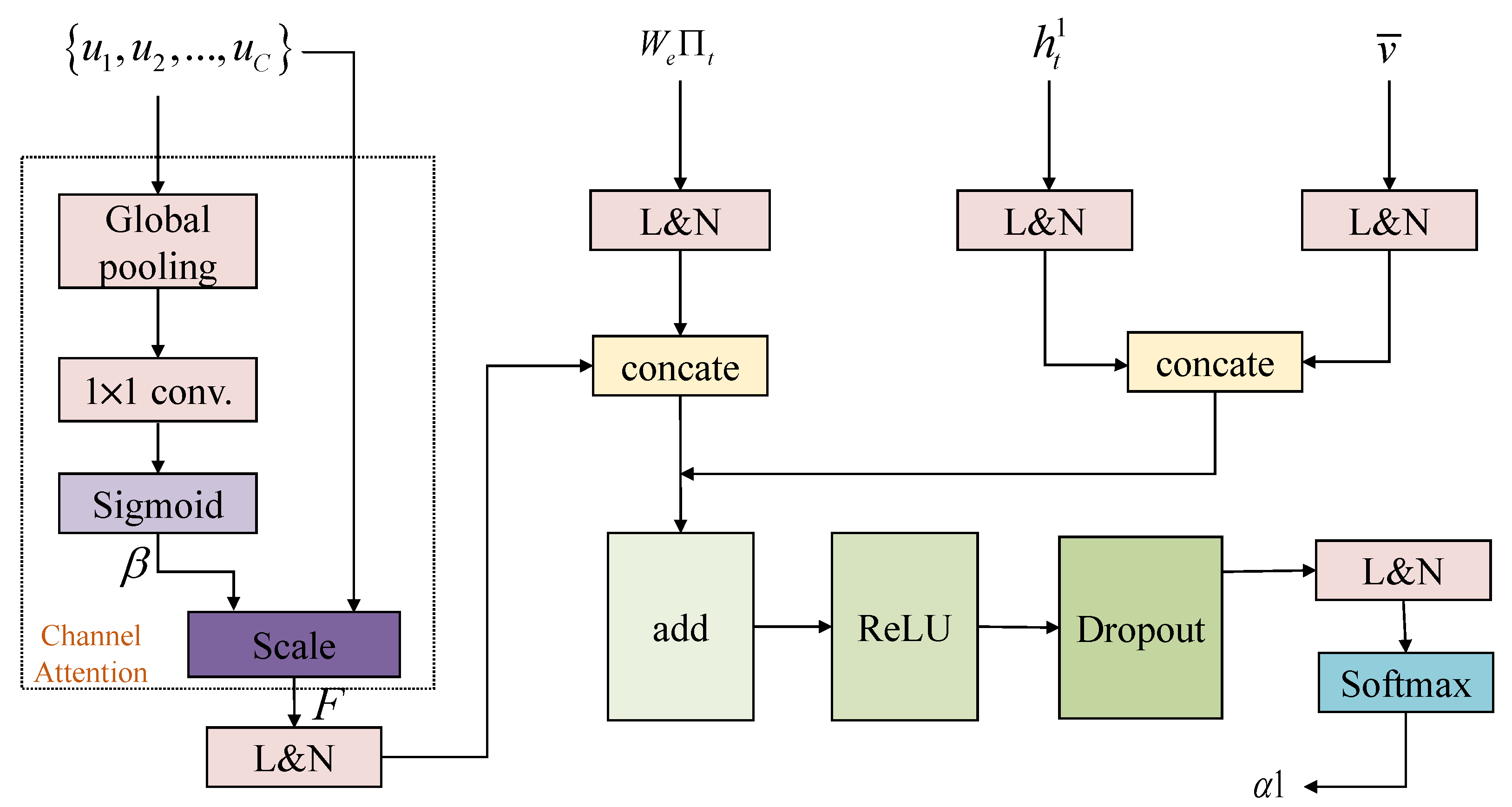
3.2. Multi-Source Interactive Attention

In the task of image captioning, the training samples provided are actually multi-source, including information from both image and text. In addition, through processing of the original training sample information, new features with clear meaning can be constructed as auxiliary information, in order to improve the performance of the model. Regarding the use of the training sample information, many current models are insufficient, resulting in unsatisfactory performance. Therefore, it is meaningful to focus on how to improve the utilization of sample information by using an attention mechanism.

The above-mentioned feature map V can also be expressed in another form:

$$U=\left\{u_1,u_2,\dots ,u_C\right\},$$

(4)

where $u_i\in R^{H\times W}$ is the feature map of the $i^{\mathrm{th}}$ channel. By calculating the mean value of the feature map of each channel respectively, $\overline{U}$ can be represented as:

$$\overline{U}=\left\{{\overline{u}}_1,{\overline{u}}_2,\dots ,{\overline{u}}_C\right\},$$

(5)

where

$${\overline{u}}_k=\frac{1}{H\times W}\sum _{i=1}^H\sum _{j=1}^W{u}_k\left(i,j\right),$$

(6)

where $u_k\left(i,j\right)$ is the value at position $(i,j)$ of the $k^{\mathrm{th}}$ channel feature $u_k$ of the feature map.

As each channel is sensitive to a certain semantic object, the mean value of the channel can also reflect the semantic feature of the corresponding object, to a certain extent. If the mean value of each channel is collected, the semantic feature of an RSI can be represented partly. Differing from the attribute attention [4], where the output of a fully connected layer or softmax layer from a CNN was used to express the semantic features of an RSI, our model uses the average of each channel to express the semantic features, thus greatly reducing the amount of parameters, which can further improve the training speed of the model. Meanwhile, in order to further utilize the channel dimension aggregation information, we use an ordinary channel attention mechanism to weight different channels, improving the response of clear and specific semantic objects in the image. In order to achieve the above objectives and to learn the non-linear interactions among channels, the channel attention weight $\beta$ calculation formula is used, as follows:

$$\beta =\sigma \left(con{v}_{1\times 1}\left(\overline{U}\right)\right),$$

(7)

where $\beta \in R^C$; $con{v}_{1\times 1}\left(·\right)$ denotes the $1\times 1$ convolution operation; and $\sigma \left(·\right)$ is the sigmoid function, which can enhance the non-linear expression of network model. Slightly different from SENet, we use $1\times 1$ convolution, instead of the FC layer in SENet.

The channel-level features F weighted by channel attention mechanism can be written as follows:

$$\begin{array}{c}F=\{f_1,f_2,\dots ,f_C\},\hfill \\ f_i={\beta }_i{u}_i.\hfill \end{array}$$

(8)

The Up-Down [21] has shown that the generated words can guide further word generation. The word information at time t is given by the following formula:

$$T_t=W_e{\mathrm{\Pi }}_t,$$

(9)

where $W_e$ denotes the word embedding matrix, and ${\mathrm{\Pi }}_t$ is the one-hot coding of input words at time t. Then, the multi-source attention weight, $\alpha 1$, can be constructed as:

$$\begin{array}{c}\alpha 1_{tc}=\mathrm{softmax}\left(w_{\alpha }^T\mathrm{ReLU}\right(\left[W_f{f}_c,unsq\left(W_T{T}_t\right)\right]\\ +unsq\left(\left[W_v\overline{v},W_h{h}_t^1\right]\right)\left)\right),\end{array}$$

(10)

where $\alpha 1_{tc}$ represents the multi-source attention weight weighted for the feature of channel c at time t; $w_{\alpha }\in R^A$, $W_f\in R^{\frac{A}{2}\times C}$, $W_T\in R^{\frac{A}{2}\times E}$, $W_v\in R^{\frac{A}{2}\times C}$, and $W_h\in R^{\frac{A}{2}\times M}$ are trainable parameters; A is the hidden layer dimension of the multi-source attention mechanism; M is the output state $h_t^1$ dimension of the multi-source LSTM; $\left[,\right]$ denotes the concatenation operation on the corresponding dimension; and $unsq\left(·\right)$ denotes expanding on the corresponding dimension, in order to make the dimension of the concatenated object consistent. The structure of multi-source interactive attention mechanism is depicted in Figure 1.

3.3. Stair Attention

The soft attention mechanism [2] processes information by treating the weighted average of N input information as the output of the attention mechanism, while the hard attention mechanism [2] randomly selects one of the N input information (i.e., the information output is the one with the highest probability). The soft attention mechanism may give more weight to multiple regions, resulting in more regions of interest and attention confusion, while the hard attention mechanism only selects one information output, which may cause great information loss and reduce the performance of the model. The above two attention mechanisms are both extreme in information selection, so we design a transitional attention mechanism to balance them.

Inspired by the physiological structure of human retinal imaging, we re-framed the approach to spatial attention weighting. There are two kinds of photoreceptors—cone cells and rod cells—in the human retina. The cone cells are mainly distributed near the central concave (fovea), but are less distributed around the retina. These cells are sensitive to the color and details of objects. Retinal ganglion neurons are the main factors of image resolution in human vision, and each cone cell can activate multiple retinal ganglion neurons. Therefore, the concentrated distribution of cone cells plays an important role in high-resolution visual observation. Some previous spatial attention mechanisms, such as soft attention mechanisms, have imitated this distribution, but the weight distribution was not very accurate. Based on the attention weights, these weights are regarded as reflecting the distribution of cone cells; therefore, the area with the largest weight can be regarded as the fovea, the cone cells around the fovea are reduced, and the cone cells far away from the fovea are more sparser. In this way, the physiological structure of human vision is imitated. As the distribution of attention weights is stair-like after classification, the attention mechanism proposed in this section is named stair attention mechanism.

After obtaining the multi-source interactive attention weights, we designed a stair attention mechanism to redistribute the weights, as shown in Figure 2, which consists of two modules: A data statistics module and a weight redistribution module.

In the data statistics module, for multi-source attention weights $\alpha 1_i\in R^{W\times H}\left(i=1\sim C\right)$, the maximum weight value $\alpha 1_{imax}$, the minimum weight value $\alpha 1_{imin}$, and the coordinates $\left(x_i,y_i\right)$ of the maximum weight value are determined as follows:

$$\begin{array}{c}\alpha 1_{i max}=MAX\left(\alpha 1_i\right),\\ \alpha 1_{i min}=MIN\left(\alpha 1_i\right),\\ \left(x_i,y_i\right)=argmax\left(\alpha 1_i\right),\end{array}$$

(11)

where $MAX\left(·\right)$, $MIN\left(·\right)$, and $argmax\left(·\right)$ represent the maximum, minimum, and maximum position functions, respectively. The weight redistribution module is used to allocate the weights of the output of the data statistics module. Taking $\alpha 1_i$ as an example, as a two-dimensional matrix, the value ranges in the wide and high dimensions are $1\sim W$ and $1\sim H$, respectively. The following three cases are based on the possible location of $\left(x_i,y_i\right)$:

(1) $\left(x_i,y_i\right)$ is located at the four corners of the feature map

$$\begin{array}{c}{\mathrm{\Delta }}_1=\left(1-\alpha 1_{i max}-\left(W\times H-1\right)\times \alpha 1_{i min}\right)/4,\hfill \\ \alpha 2_i\left(w,h\right)=\left\{\begin{array}{c}\alpha 1_{i max}+{\mathrm{\Delta }}_{1}w=x_i,h=y_i\hfill \\ \alpha 1_{i min}+{\mathrm{\Delta }}_{1}w\in U\left(x_i,3\right)\bigcap \left[1,W\right],h\in U\left(y_i,3\right)\bigcap \left[1,H\right],\hfill \\ \alpha 1_{i min}others\hfill \end{array}\right.\hfill \end{array}$$

(12)

In the above formula, $\alpha 2_i\left(w,h\right)$ represents the weight corresponding to the position $\left(w,h\right)$ of the $i^{\mathrm{th}}$ channel of the stair attention weight $\alpha 2$, $U\left(k,\delta \right)$ represents the weight of the $\delta$-neighborhood of k, and ⋂ is the union symbol (similarly below). The reason for dividing ${\mathrm{\Delta }}_1$ by 4 is that there are only four elements in the $\alpha 1_i$ matrix in the 3-neighborhood of $\left(x_i,y_i\right)$.

(2) $\left(x_i,y_i\right)$ is on the edge of the feature map

$$\begin{array}{c}{\mathrm{\Delta }}_2=\left(1-\alpha 1_{i max}-\left(W\times H-1\right)\times \alpha 1_{i min}\right)/6,\hfill \\ \alpha 2_i\left(w,h\right)=\left\{\begin{array}{c}\alpha 1_{i max}+{\mathrm{\Delta }}_{2}w=x_i,h=y_i\hfill \\ \alpha 1_{i min}+{\mathrm{\Delta }}_{2}w\in U\left(x_i,3\right)\bigcap \left[1,W\right],h\in U\left(y_i,3\right)\bigcap \left[1,H\right],\hfill \\ \alpha 1_{i min}others\hfill \end{array}\right.\hfill \end{array}$$

(13)

There are six elements in the $\alpha 1_i$ matrix in the 3-neighborhood of $\left(x_i,y_i\right)$.

(3) Other cases

$$\begin{array}{c}{\mathrm{\Delta }}_3=\left(1-\alpha 1_{i max}-\left(W\times H-1\right)\times \alpha 1_{i min}\right)/9,\hfill \\ \alpha 2_i\left(w,h\right)=\left\{\begin{array}{c}\alpha 1_{i max}+{\mathrm{\Delta }}_{3}w=x_i,h=y_i\hfill \\ \alpha 1_{i min}+{\mathrm{\Delta }}_{3}w\in U\left(x_i,3\right)h\in U\left(y_i,3\right),\hfill \\ \alpha 1_{i min}others\hfill \end{array}\right.\hfill \end{array}$$

(14)

There are nine elements in the $\alpha 1_i$ matrix in the 3-neighborhood of $\left(x_i,y_i\right)$. The reason why 1 is subtracted in the above three cases is to ensure that the weight of all elements in the feature map is 1.

The stair attention weights for the above three cases are shown in Figure 3. The blue region is the region with the lowest weight (i.e., the first stair). The pink area is the area with the second lowest weight (i.e., the second stair). The red area is the highest weight area (i.e., the third stair). The third stair is the area of the most concern, which can be compared to the distribution of cone cells in the fovea of the human retina. The second stair is used to simulate the distribution of cone cells around the fovea, where the attention is weaker, but can assist the third stair. As the first stair is far away from the third stair, the attention weight of the first stair is set to the lowest, and less resources are spent here.

After the stair attention weight $\alpha 2$ is obtained, the final feature output after attention weighting is obtained using the following formula:

$$\begin{array}{c}{\widehat{v}}_t={\displaystyle \sum _{i=1}^K}{\alpha }_{ti}{v}_i,\hfill \\ \alpha =\alpha 1+\alpha 2.\hfill \end{array}$$

(15)

3.4. Captioning Model

The decoder adopts the same strategy as the Up-Down [21], using a two-layer LSTM architecture. The first LSTM, called multi-source LSTM, receives multi-source information. The second LSTM is called language LSTM, and is responsible for generating descriptions. In the following equation, superscript 1 is used to represent multi-source LSTM, while superscript 2 represents language LSTM. The following formula is used to describe the operation of the LSTM at time t:

$$h_t=LSTM\left(x_t,h_{t-1}\right),$$

(16)

where $x_t$ is the LSTM input vector and $h_t$ is the output vector. For convenience, the transfer process of memory cells in LSTM is omitted here. The overall model framework is shown in Figure 4.

(1) Multi-source LSTM: As the first LSTM, the multi-source LSTM receives information from the encoder, including the state information $h_{t-1}^2$ of the last step of the language LSTM, the mean value $\overline{v}$ of the image feature representation, and the word information $W_e{\mathrm{\Pi }}_t$ at the current time step. The input vector can be expressed as:

$$x_t^1=\left[h_{t-1}^2,\overline{v},W_e{\mathrm{\Pi }}_t\right].$$

(17)

(2) Language LSTM: The input of language LSTM includes the output of the stair attention module and the output of the multi-source LSTM. It can be expressed by the following formula:

$$x_t^2=\left[{\widehat{v}}_t,h_t^1\right],$$

(18)

where $y_{1:L}$ represents the word sequence $\left(y_1,\dots ,y_L\right)$. At each time t, the conditional probability of possible output words is as follows:

$$p\left(y_t\left|y_{1:t-1}\right.\right)=\mathrm{softmax}\left(W_p{h}_t^2+b_p\right),$$

(19)

where $W_p\in R^{\left|\mathrm{\Sigma }\right|\times M}$ and $b_p\in R^{\left|\mathrm{\Sigma }\right|}$ are learnable weights and biases. The probability distribution on the complete output sequence is calculated through multiplication of the conditional probability distribution:

$$p\left(y_{1:L}\right)=\prod _{t=1}^{L}p\left(y_t\left|y_{1:t-1}\right.\right).$$

(20)

3.5. Training Strategy

During captioning training, the prediction of words at time t is conditioned on the preceding words ($y_{1:t-1}$). Given the annotated caption, the confidence of the prediction $y_t$ is optimized by minimizing the negative log-likelihood over the generated words:

$$los{s}_{\mathrm{CE}}^{\theta }=\frac{1}{T}\sum _{t=1}^T-log\left(p_t^{\theta }\left(y_t\left|y_{1:t-1},V\right.\right)\right),$$

(21)

where $\theta$ denotes all learned parameters in the captioning model. Following previous works [15], after a pre-training step using CE, we further optimize the sequence generation through RL-based training. Specifically, we use the SCST [43] to estimate the linguistic position of each semantic word, which is optimized for the CIDEr-D metric, with the reward obtained under the inference model at training time:

$$los{s}_{RL}^{\theta }=-E_{\omega 1:T\sim \theta }\left[r\left({\omega }_{1:T}\right)\right],$$

(22)

where r is the CIDEr-D score of the sampled sentence ${\omega }_{1:T}$. The gradient of $los{s}_{RL}^{\theta }$ can be approximated by Equation (23), where $r\left({\omega }_{1:T}^s\right)$ and $r\left({\widehat{\omega }}_{1:T}\right)$ are the CIDEr rewards for the random sampled sentence and the max sampled sentence, respectively.

$${\nabla }_{\theta }los{s}_{RL}^{\omega }=-\left(r\left({\omega }_{1:T}^s\right)-r\left({\widehat{\omega }}_{1:T}\right)\right){\nabla }_{\theta }log\left(p^{\omega }\left({\omega }_{1:T}^s\right)\right).$$

(23)

4. Experiments and Analysis

4.1. Data Set and Setting

4.1.1. Data Set

In this paper, three public data sets are used to generate the descriptions for RSIs. The details of the three data sets are provided in the following.

(1)

RSICD [3]: All the images in RSICD data set are from Google Earth, and the size of each image is $224\times 224$ pixels. This data set contains 10,921 images, each of which is manually labeled with five description statements. The RSICD data set is the largest data set in the field of RSIC. There are 30 kinds of scenes in RSICD.

(2)

UCM-Captions [33]: The UCM-Captions data set is based on the UC Merced (UCM) land-use data set [46], which provides five description statements for each image. This data set contains 2100 images of 21 types of features, including runways, farms, and dense residential areas. There are 100 pictures in each class, and the size of each picture is $256\times 256$ pixels. All the images in this data set were captured from the large image of the city area image from the national map of the U.S. Geological Survey.

(3)

Sydney-Captions [33]: The Sydney captions data set is based on the Sydney data set [47], providing five description statements for each picture. This data set contains 613 images with 7 types of ground objects. The size of each image is $500\times 500$ pixels.

4.1.2. Evaluation Metrics

Researchers have proposed several evaluation metrics to judge whether a description generated by a machine is good or not. The most commonly used metrics for the RSIC task include BLEU-n [48], METEOR [49], ROUGE_L [50], and CIDEr [51], which are used as evaluation metrics to verify the effectiveness of a model. BLEU-n scores ($n=$ 1, 2, 3, or 4) represents the precision ratio by comparing the generated sentence with reference sentences. Based on the harmonic mean of uniform precision and recall, the METEOR score reflects the precision and recall ratio of the generated sentence. ROUGE_L captures semantic quality by comparing scene graphs. The scene graph turns each component of each tuple (i.e., object, object–attribute, subject–relationship–object) into a node. CIDEr measures consistency between n-gram occurrences in generated and reference sentences, where the consistency is weighted by n-gram saliency and rarity.

4.1.3. Training Details and Experimental Setup

In our experiments, VGG16 was used to extract appearance features, which is pre-trained on the ImageNet data set [52]. Note that the size of the output feature maps from the last layer of VGG16 is $14\times 14\times 512$.

For three public data sets, the proportion of training, validation, and test sets in the three data sets were 80%, 10%, and 10%, respectively. All RSIs were cropped to a size of $224\times 224$ before being input to the model. In practice, all the experiments, including the fine-tuning encoder process and the decoder training process, were carried out on a server with an NVIDIA GeForce GTX 1080Ti. The hidden state size of the two LSTMs was 512. Every word in the sentence was also represented as a 512-dimensional vector. Each selected region was described with such a 512-dimensional feature vector. The initial learning rates of the encoder and decoder were set to $1\times {10}^{-5}$ and $5\times {10}^{-4}$, respectively. The mini-batch size was 64. We set the maximum number of training iterations as 35 epochs. In order to obtain better captions, the beam search algorithm was applied during the inference period, with the number of beams equal to 3.

4.1.4. Compared Models

In order to evaluate our model, we compared it with several other state-of-the-art approaches, which exploit either spatial or multi-task driven attention structures. We first briefly review these methods in the following.

(1)

SAT [3]: A architecture that adopts spatial attention to encode an RSI by capturing reliable regional features.

(2)

FC-Att/SM-Att [4]: In order to utilize the semantic information in the RSIs, this method updates the attentive regions directly, as related to attribute features.

(3)

Up-Down [21]: A captioning method that considers both visual perception and linguistic knowledge learning to generate accurate descriptions.

(4)

LAM [39]: A RSIC algorithm based on the scene classification task, which can generate scene labels to better guide sentence generation.

(5)

MLA [34]: This method utilizes a multi-level attention-based RSIC network, which can capture the correspondence between each candidate word and image.

(6)

Sound-a-a [40]: A novel attention mechanism, which uses the interaction of the knowledge distillation from sound information to better understand the RSI scene.

(7)

Struc-Att [37]: In order to better integrate irregular region information, a novel framework with structured attention was proposed.

(8)

Meta-ML [38]: This model is a multi-stage model for the RSIC task. The representation for a given image is obtained using a pre-trained autoencoder module.

4.2. Evaluation Results and Analysis

We compared our proposed MSISAM with a series of state-of-the-art RSIC approaches on three different data sets: Sydney-Captions, UCM-Captions, and RSICD. Specifically, for the MSISAM model, we utilized the VGG16-based encoder for visual features and followed reinforcement learning techniques in the training step.

Table 1. Comparison of scores for our method and other state-of-the-art methods on the Sydney-Captions data set [33].

Methods	Bleu1	Bleu2	Bleu3	Bleu4	Meteor	Rouge	Cider
SAT [3]	0.7905	0.7020	0.6232	0.5477	0.3925	0.7206	2.2013
FC-Att [4]	0.8076	0.7160	0.6276	0.5544	0.4099	0.7114	2.2033
SM-Att [4]	0.8143	0.7351	0.6586	0.5806	0.4111	0.7195	2.3021
Up-Down [21]	0.8180	0.7484	0.6879	0.6305	0.3972	0.7270	2.6766
LAM [39]	0.7405	0.6550	0.5904	0.5304	0.3689	0.6814	2.3519
MLA [34]	0.8152	0.7444	0.6755	0.6139	0.4560	0.7062	1.9924
sound-a-a [40]	0.7484	0.6837	0.6310	0.5896	0.3623	0.6579	2.7281
Struc-Att [37]	0.7795	0.7019	0.6392	0.5861	0.3954	0.7299	2.3791
Meta-ML [38]	0.7958	0.7274	0.6638	0.6068	0.4247	0.7300	2.3987
Ours(SCST)	0.7643	0.6919	0.6283	0.5725	0.3946	0.7172	2.8122

,

Table 2. Comparison of scores for our method and other state-of-the-art methods on the UCM-Captions data set [33].

Methods	Bleu1	Bleu2	Bleu3	Bleu4	Meteor	Rouge	Cider
SAT [3]	0.7993	0.7355	0.6790	0.6244	0.4174	0.7441	3.0038
FC-Att [4]	0.8135	0.7502	0.6849	0.6352	0.4173	0.7504	2.9958
SM-Att [4]	0.8154	0.7575	0.6936	0.6458	0.4240	0.7632	3.1864
Up-Down [21]	0.8356	0.7748	0.7264	0.6833	0.4447	0.7967	3.3626
LAM [39]	0.8195	0.7764	0.7485	0.7161	0.4837	0.7908	3.6171
MLA [34]	0.8406	0.7803	0.7333	0.6916	0.5330	0.8196	3.1193
sound-a-a [40]	0.7093	0.6228	0.5393	0.4602	0.3121	0.5974	1.7477
Struc-Att [37]	0.8538	0.8035	0.7572	0.7149	0.4632	0.8141	3.3489
Meta-ML [38]	0.8714	0.8199	0.7769	0.7390	0.4956	0.8344	3.7823
Ours(SCST)	0.8727	0.8096	0.7551	0.7039	0.4652	0.8258	3.7129

and

Table 3. Comparison of scores for our method and other state-of-the-art methods on the RSICD data set [3].

Methods	Bleu1	Bleu2	Bleu3	Bleu4	Meteor	Rouge	Cider
SAT [3]	0.7336	0.6129	0.5190	0.4402	0.3549	0.6419	2.2486
FC-Att [4]	0.7459	0.6250	0.5338	0.4574	0.3395	0.6333	2.3664
SM-Att [4]	0.7571	0.6336	0.5385	0.4612	0.3513	0.6458	2.3563
Up-Down [21]	0.7679	0.6579	0.5699	0.4962	0.3534	0.6590	2.6022
LAM [39]	0.6753	0.5537	0.4686	0.4026	0.3254	0.5823	2.5850
MLA [34]	0.7725	0.6290	0.5328	0.4608	0.4471	0.6910	2.3637
sound-a-a [40]	0.6196	0.4819	0.3902	0.3195	0.2733	0.5143	1.6386
Struc-Att [37]	0.7016	0.5614	0.4648	0.3934	0.3291	0.5706	1.7031
Meta-ML [38]	0.6866	0.5679	0.4839	0.4196	0.3249	0.5882	2.5244
Ours(SCST)	0.7836	0.6679	0.5774	0.5042	0.3672	0.6730	2.8436

detail the performance of our model and other attention-based models on the Sydney-Captions, UCM-Captions, and RSICD data sets, respectively. It can be clearly seen that our model presented superior performance over the compared models in almost all of the metrics. The best results of all algorithms, using the same encoder, are marked in bold.

Quantitative Comparison: First, can be seen, the SAT obtained the lowest scores in Table 1, Table 2 and Table 3, which was expected, as it only uses CNN–RNN without any modifications or additions. It is worth mentioning that attribute-based attention mechanisms are utilized in FC-Att, SM-Att, and LAM. Compared with SAT, adopting attribute-based attention in the RSIC task improved the performance in all evaluation metrics (i.e., BLEU-n, METEOR, ROUGE-L, and CIDEr). The LAM obtained a high CIDEr score on UCM-Captions and a low BLEU-4 score on Sydney-Captions. This reveals that the UCM-Captions provides a larger vocabulary than Sydney-Captions. However, for the RSICD data set, whose larger-scale data and vocabulary may bring more difficulties in training the models, the improvement was quite limited. The results of all models on the UCM-Captions data set are shown in Table 2. The MLA model performed slightly better than our models in the METEOR and ROUGE metrics; however, the performance of MLA on the Sydney-Captions and RSICD data sets was not competitive.

To some extent, RSIC models with multi-task assistance have gradually been put forward (i.e., Sound-a-a, Struc-Att, Meta-ML). Extra sound information is provided in Sound-a-a, which led to performance improvements. On Sydney-Captions, the semantic information was the most scarce. As shown in Table 1, Sound-a-a consistently outperformed most methods in the CIDEr metric. In particular, the CIDEr score of Sound-a-a reached an absolute improvement of 5.15% against the best competitor (Up-Down). Struc-Att takes segmented irregular areas as visual inputs. The results of Struct-attention in Table 1, Table 2 and Table 3 also demonstrate that obtaining object structure features is useful. However, in some cases, it presented worse performance (i.e., on RSICD). This is because the complex objects and 30 land categories in RSICD weakened the effectiveness of the segmentation block. To extract image features considering the characteristics in RSIs, meta learning is applied in Meta-ML, which could capture the strong grid features. In this way, as shown in Table 1, Table 2 and Table 3, a significant improvement was obtained in all other metrics on the three data sets. Thus, we consider that high-quality visual features provide convenient visual semantic transformation.

In addition, we observed that the Up-Down model served as a strong baseline for attention-based models. Up-Down utilizes double LSTM-based structures to trigger bottom-up and top-down attention, leading to clear performance boosts. The results of the Up-Down obtained showed better BLEU-n scores on the Sydney-Captions data set. Upon adding the MSISAM in our model, the performance was further improved, compared to using only CNN features and spatial attention. When we added the refinement module (Ours*), we observed a slight degradation in the other evaluation metrics (BLUE-n, METEOR, and ROUGE-L). However, the CIDEr evaluation metric showed an improvement. As can be seen from the results, the effectiveness of Ours* was confirmed, with improvements of 13.56% (Sydney-Captions), 9.58% (UCM-Captions), and 24.14% (RSICD) in CIDEr, when compared to the Up-Down model. Additionally, we note that our model obtained competitive performance, compared to other state-of-the-art approaches, surpassing them in all evaluation metrics.

Qualitative Comparison: In Figure 5, examples of RSI content descriptions are shown, from which it can be seen that the MSISAM captured more image details than the Up-Down model. This phenomenon demonstrates that the attentive features extracted by multi-source interaction with the stair attention mechanism can effectively enhance the content description. The introduction of multi-source information made the generated sentences more detailed. It is worth mentioning that the stair attention has the ability to reallocate weights on the visual features dynamically at each time step.

As shown in Figure 5a, the Up-Down model ignored the scenario information of “blue sea” and “white sands”, while our proposed model identified the scene correctly in the image, describing the color attributes of the sea and sand. For the scene “playground”, as the main element of the image in Figure 5e, the “playground” was incorrectly described as a “railway station” by the Up-Down model. MSISAM also improved the coherence of the paragraph by explicitly modeling topic transition. As seen from Figure 5d, it organized the relationship between “marking lines” and “runways” with “on”. At the same time, Figure 5b shows that the MSISAM can describe small objects (i.e., “cars”) in the figure. In addition, we found, from Figure 5f, that the sentences generated by Up-Down make it difficult to obtain accurate quantitative information. Although the sentence reference provides accurate quantitative knowledge, our model can tackle this problem and generated an accurate caption (“four baseball fields”). It is worth noting that the proposed model sometimes generated more appropriate sentences than the manually marked references: as shown in Figure 5c, some “roads” in the “industrial area” are also described. The above examples prove that the proposed model can further improve the ability to describe RSIs. In addition, Figure 6 shows the image regions highlighted by the stair attention. For each generated word, we visualized the attention weights for individual pixels, outlining the region with the maximum attention weight in orange. From Figure 6, we can see that the stair attention was able to locate the right objects, which enables it to accurately describe objects in the input RSI. On the other hand, the visual weights were obviously higher when our model predicted words related to objects (e.g., “baseball field” and “bridge”).

4.3. Ablation Experiments

Next, we conducted ablation analyses regarding the coupling of the proposed MSIAM, MSISAM, and the combination of the latter with SCST. For convenience, we denote these models as A2, A3, and A4, respectively. Please note that all the ablation studies were conducted based on the VGG16 encoder.

(1)

Baseline (A1): The baseline [21] was formed by VGG16 combined with two LSTMs.

(2)

MSIAM (A2): A2 denotes the enhanced model based on the Baseline, which utilizes the RSI semantics from sentence fragments and visual features.

(3)

MSISAM (A3): Integrating multi-source interaction with stair attention, A3 can highlight the most concerned image areas.

(4)

With SCST (A4): We trained the A3 model using the SCST and compared it with the performance obtained by the CE.

Quantitative Comparison: For the A1, A2, and A3 models, the scores shown in

Table 4. Ablation performance of our designed model on the Sydney-Captions data set [33].

Methods	Bleu1	Bleu2	Bleu3	Bleu4	Meteor	Rouge	Cider
A1	0.8180	0.7484	0.6879	0.6305	0.3972	0.7270	2.6766
A2	0.7995	0.7309	0.6697	0.6108	0.3983	0.7303	2.7167
A3	0.7918	0.7314	0.6838	0.6412	0.4079	0.7281	2.7485
A4	0.7643	0.6919	0.6283	0.5725	0.3946	0.7172	2.8122

,

Table 5. Ablation performance of our designed model on the UCM-Captions data set [33].

Methods	Bleu1	Bleu2	Bleu3	Bleu4	Meteor	Rouge	Cider
A1	0.8356	0.7748	0.7264	0.6833	0.4447	0.7967	3.3626
A2	0.8347	0.7773	0.7337	0.6937	0.4495	0.7918	3.4341
A3	0.8500	0.7923	0.7438	0.6993	0.4573	0.8126	3.4698
A4	0.8727	0.8096	0.7551	0.7039	0.4652	0.8258	3.7129

and

Table 6. Ablation performance of our designed model on the RSICD data set [3].

Methods	Bleu1	Bleu2	Bleu3	Bleu4	Meteor	Rouge	Cider
A1	0.7679	0.6579	0.5699	0.4962	0.3534	0.6590	2.6022
A2	0.7711	0.6645	0.5777	0.5048	0.3574	0.6674	2.7288
A3	0.7712	0.6636	0.5762	0.5020	0.3577	0.6664	2.6860
A4	0.7836	0.6679	0.5774	0.5042	0.3672	0.6730	2.8436

are under CE training, while those for the A4 model are with SCST training. Interestingly, ignoring the semantic information undermined the performance of the Baseline, verifying our hypothesis that the interaction between linguistic and visual information benefits cross-modal transition. A2 could function effectively, regarding the integration of semantics from generated linguistics. However, the improvement was not obvious for our A2 model combined with the designed channel attention, which learns semantic vectors from visual features. From the results of A3, we utilized the stair attention to construct a closer mapping relationship between images and texts, where A3 reduces the difference among the distributions of semantic vector and attentive vector at different time steps. As for diversity, the replacement-based reward enhanced the sentence-level coherence. As can be seen in Table 4, Table 5 and Table 6, the use of the CIDEr metric led to great success, as the increment-based reward promoted sentence-level accuracy. Thus, higher scores were achieved when A3 was trained with SCST.

Qualitative Comparison: We show the descriptions generated by GT, the Baseline (A1), MSIAM (A2), MSISAM (A3), and our full model (A4) in Figure 7. In Figure 7a, the word is incorrectly included in captions (i.e., “stadium”) from Baseline, likely due to a stereotype. Regarding such cases, A3 and A4, using the specific semantic heuristic, may determine the correlation between a word’s most related regions. The “large white building” and “roads” could be described in the scene by A3 and A4. Figure 7e is similar to Figure 7a, where the “residential area” in the description is not correlated with the image topic. Another noteworthy point is that the logical relationship between “buildings” and “park” was disordered by A2. We extended the A2 with SCST to mine the sentence-level coherence for boosting sentence generation (i.e., a “Some buildings are near a park with many green trees and a pond”). As shown in Figure 7d, the caption generated by A4 was accurate, as well as containing clear and coherent grammatical structure. The stair attention in A3 acts more smoothly and allows for better control of the generated descriptions. In Figure 7c, where the caption should include “two bridges”, this information was not captured by A1 or A2, as inferring such content requires the amount of contextual and historical knowledge that can be learned by A3 and A4.

Despite the high quality of the captions for most of the RSIs, there were also some examples of failures illustrated in Figure 7. Some objects in the generated caption were not in the image. There were no schools in Figure 7b, but the word “school” was included in all of the final descriptions. This may be due to the high frequency of some words in the training data. Figure 7f shows another example of misrecognition. Many factors contribute to this problem, such as the color or appearance of objects. The “resort” generated by A1 and A2 shared the same color with the roof of the “building”. In A3 and A4, the “storage tanks” and “river” share the similar appearance with the roof of “building”. This is still an open challenge in the RSIC field. Enabling models to predict the appropriate words through the aid of external knowledge and common sense may help to alleviate this problem.

4.4. Parameter Analysis

In order to evaluate the influence of adopting different CNN features for the generation of sentences, experiments based on different CNN architectures were conducted. In particular, VGG16, VGG19, ResNet50, and ResNet101 were adopted as encoders. Note that, with the different CNN structures, the size of the output feature maps of the last layer of the CNN network also differs. The size of the extracted features from the VGG networks is $14\times 14\times 512$, while the feature size was $7\times 7\times 2048$ with the ResNet networks. In

Table 7. Comparison experiments on Sydney-Captions data set [33] based on different CNNs.

Methods	Encoder	Bleu1	Bleu2	Bleu3	Bleu4	Meteor	Rouge	Cider
VGG16	Up-Down	0.8180	0.7484	0.6879	0.6305	0.3972	0.7270	2.6766
	MSISAM	0.7918	0.7314	0.6838	0.6412	0.4079	0.7281	2.7485
VGG19	Up-Down	0.7945	0.7231	0.6673	0.6188	0.4109	0.7360	2.7449
	MSISAM	0.8251	0.7629	0.7078	0.6569	0.4185	0.7567	2.8334
ResNet50	Up-Down	0.7568	0.6745	0.6130	0.5602	0.3763	0.6929	2.4212
	MSISAM	0.7921	0.7236	0.6647	0.6111	0.3914	0.7113	2.4501
ResNet101	Up-Down	0.7712	0.6990	0.6479	0.6043	0.4078	0.6950	2.4777
	MSISAM	0.7821	0.7078	0.6528	0.6059	0.4078	0.7215	2.5882

,

Table 8. Comparison experiments on the UCM-Captions data set [33] based on different CNNs.

Methods	Encoder	Bleu1	Bleu2	Bleu3	Bleu4	Meteor	Rouge	Cider
VGG16	Up-Down	0.8356	0.7748	0.7264	0.6833	0.4447	0.7967	3.3626
	MSISAM	0.8500	0.7923	0.7438	0.6993	0.4573	0.8126	3.4698
VGG19	Up-Down	0.8317	0.7683	0.7205	0.6779	0.4457	0.7837	3.3408
	MSISAM	0.8469	0.7873	0.7373	0.6908	0.4530	0.8006	3.4375
ResNet50	Up-Down	0.8536	0.7968	0.7518	0.7122	0.4643	0.8111	3.5591
	MSISAM	0.8621	0.8088	0.7640	0.7231	0.4684	0.8126	3.5774
ResNet101	Up-Down	0.8545	0.8001	0.7516	0.7067	0.4635	0.8147	3.4683
	MSISAM	0.8562	0.8011	0.7531	0.7086	0.4652	0.8134	3.4686

and

Table 9. Comparison experiments on the RSICD data set [3] based on different CNNs.

Methods	Encoder	Bleu1	Bleu2	Bleu3	Bleu4	Meteor	Rouge	Cider
VGG16	Up-Down	0.7679	0.6579	0.5699	0.4962	0.3534	0.6590	2.6022
	MSISAM	0.7712	0.6636	0.5762	0.5020	0.3577	0.6664	2.6860
VGG19	Up-Down	0.7550	0.6383	0.5466	0.4697	0.3556	0.6533	2.5350
	MSISAM	0.7694	0.6587	0.5715	0.4986	0.3613	0.6629	2.6631
ResNet50	Up-Down	0.7687	0.6505	0.5577	0.4818	0.3565	0.6607	2.5924
	MSISAM	0.7785	0.6631	0.5704	0.4929	0.3648	0.6665	2.6422
ResNet101	Up-Down	0.7685	0.6555	0.5667	0.4920	0.3561	0.6574	2.5601
	MSISAM	0.7785	0.6694	0.5809	0.5072	0.3603	0.6692	2.7027

, we report the performance of Up-Down and our proposed models on the three public data sets, respectively. The best results of the three different algorithms with the same encoder are marked in bold.

Table 7 details the impact of adopting different CNNs as encoders on the Sydney-Captions data set. The experiments showed that VGG16 or VGG19 performed better as encoders than the ResNet networks. Overall, our MSISAM with VGG19 showed the best performance, compared with Up-Down. Comparing the VGG19 and ResNet101 encoders applied to the MSISAM, BLEU-$1\sim 4$ were greatly improved, as well as CIDEr, which increased by 9.5%. The experimental results on UCM-Captions are shown in Table 8. MSISAM surpassed Up-Down, in terms of most metrics, with ResNet networks as encoders; of which, ResNet50 was the better choice as an encoder. The results on RSICD are reported in Table 9. We can see that the results based on the four different CNN variants were relatively close, unlike those for Sydney-Captions and UCM-Captions. However, VGG16 and ResNet101 performed better, in terms of all metrics.

Obviously, integrating an excellent CNN backbone with our model provides much better performance than when using the unfiltered model. As indicated by our results, it is suitable to select an easy training encoder with small scale for Sydney-Captions and UCM-Captions. Sydney-Captions is the smallest data set for the RSIC task and, so, VGG-based encoders perform much better than ResNet-based encoders. However, this phenomenon was not obvious on the most complicated data set, RSICD.

We also compared the training time and inference speed (images per second) of our model with those of Up-Down model on the RSICD data set. The comparison results are shown in

Table 10. Comparison between MSISAM and Up-Down, in terms of training time and inference speed (images per second).

Methods	Training Time	Inference Speed (Images per Second)
Up-Down	253 min	16.66
MSISAM	217 min	16.78

. In particular, the training time and inference speed were tested on single NVIDIA GeForce GTX 1080Ti GPU, and the CNN framework was VGG16 in both of the models. Due to the superiority of the MSISAM, less time was used in the training process. In addition, due to the higher number of parameters in the stair attention, the inference time was slightly higher than that for the Up-Down model.

5. Conclusions

In this work, we delved into the idea of comprehending and ordering the rich semantics in RSIs for the RSIC task. To verify our claim, we present a new attention-based encoder–decoder structure—that is, multi-source interaction and stair attention—which unifies the two processes of enriched semantic information and learnable ordering regions into a single architecture. The proposed model can generate sentences with high accuracy and diversity. Particularly, the multi-source interaction module is initially utilized to accumulate the primary semantic cues implied in the preceding sentences. Next, the proposed stair attention mechanism filters out irrelevant visual regions with primary semantic cues, while inferring the relevant semantic words that are worth mentioning with respect to the visual content. Subsequently, a CIDEr-based reward is used for learning, in order to estimate the linguistic position of each semantic word, leading to a sequence of diverse semantic words. The CIDEr-based reward serves as a supervisory signal guiding sentence generation. Our experimental results showed that our model can exhibit a competitive performance on the Sydney-Captions, UCM-Captions, and RSICD data sets. We also plan to apply our model to MindSpore [53], which is a new deep learning computing framework, as future work.

References

1. Vinyals, O.; Toshev, A.; Bengio, S.; Erhan, D. Show and tell: A neural image caption generator. In Proceedings of the IEEE Conference on Computer Vision and Pattern Recognition, Boston, MA, USA, 7–12 June 2015; pp. 3156–3164. [Google Scholar]
2. Xu, K.; Ba, J.; Kiros, R.; Cho, K.; Courville, A.; Salakhudinov, R.; Zemel, R.; Bengio, Y. Show, attend and tell: Neural image caption generation with visual attention. In Proceedings of the International Conference on Machine Learning, Lille, France, 6–11 July 2015; pp. 2048–2057. [Google Scholar]
3. Lu, X.; Wang, B.; Zheng, X.; Li, X. Exploring models and data for remote sensing image caption generation. IEEE Trans. Geosci. Remote Sens. 2018, 56, 2183–2195. [Google Scholar] [CrossRef] [Green Version]
4. Zhang, X.; Wang, X.; Tang, X.; Zhou, H.; Li, C. Description generation for remote sensing images using attribute attention mechanism. Remote Sens. 2019, 11, 612. [Google Scholar] [CrossRef] [Green Version]
5. Maggiori, E.; Tarabalka, Y.; Charpiat, G.; Alliez, P. Convolutional neural networks for large-scale remote-sensing image classification. IEEE Trans. Geosci. Remote Sens. 2016, 55, 645–657. [Google Scholar] [CrossRef] [Green Version]
6. Cheng, G.; Yang, C.; Yao, X.; Guo, L.; Han, J. When deep learning meets metric learning: Remote sensing image scene classification via learning discriminative CNNs. IEEE Trans. Geosci. Remote Sens. 2018, 56, 2811–2821. [Google Scholar] [CrossRef]
7. Lu, X.; Zheng, X.; Yuan, Y. Remote sensing scene classification by unsupervised representation learning. IEEE Trans. Geosci. Remote Sens. 2017, 55, 5148–5157. [Google Scholar] [CrossRef]
8. Han, X.; Zhong, Y.; Zhang, L. An efficient and robust integrated geospatial object detection framework for high spatial resolution remote sensing imagery. Remote Sens. 2017, 9, 666. [Google Scholar] [CrossRef] [Green Version]
9. Zhang, L.; Zhang, Y. Airport detection and aircraft recognition based on two-layer saliency model in high spatial resolution remote-sensing images. IEEE J. Sel. Top. Appl. Earth Obs. Remote Sens. 2016, 10, 1511–1524. [Google Scholar] [CrossRef]
10. Zheng, Z.; Zhong, Y.; Wang, J.; Ma, A. Foreground-aware relation network for geospatial object segmentation in high spatial resolution remote sensing imagery. In Proceedings of the IEEE/CVF Conference on Computer Vision and Pattern Recognition, Seattle, WA, USA, 13–19 June 2020; pp. 4096–4105. [Google Scholar]
11. Li, X.; He, H.; Li, X.; Li, D.; Cheng, G.; Shi, J.; Weng, L.; Tong, Y.; Lin, Z. PointFlow: Flowing semantics through points for aerial image segmentation. In Proceedings of the IEEE/CVF Conference on Computer Vision and Pattern Recognition, Nashville, TN, USA, 20–25 June 2021; pp. 4217–4226. [Google Scholar]
12. Ren, Z.; Gou, S.; Guo, Z.; Mao, S.; Li, R. A mask-guided transformer network with topic token for remote sensing image captioning. Remote Sens. 2022, 14, 2939. [Google Scholar] [CrossRef]
13. Fu, K.; Li, Y.; Zhang, W.; Yu, H.; Sun, X. Boosting memory with a persistent memory mechanism for remote sensing image captioning. Remote Sens. 2020, 12, 1874. [Google Scholar] [CrossRef]
14. Zeiler, M.D.; Fergus, R. Visualizing and understanding convolutional networks. In Proceedings of the European Conference on Computer Vision, Zurich, Switzerland, 6–12 September 2014; pp. 818–833. [Google Scholar]
15. Vaswani, A.; Shazeer, N.; Parmar, N.; Uszkoreit, J.; Jones, L.; Gomez, A.; Kaiser, L.; Polosukhin, I. Attention is all you need. Proc. Adv. Neural Inf. Process. Syst. 2017, 30, 5998–6008. [Google Scholar]
16. Yohanandan, S.; Song, A.; Dyer, A.G.; Tao, D. Saliency preservation in low-resolution grayscale images. In Proceedings of the European Conference on Computer Vision (ECCV), Munich, Germany, 8–14 September 2018; pp. 235–251. [Google Scholar]
17. Graves, A. Long short-term memory. In Supervised Sequence Labelling with Recurrent Neural Networks; Springer: Berlin/Heidelberg, Germany, 2012; pp. 37–45. [Google Scholar]
18. Mao, J.; Xu, W.; Yang, Y.; Wang, J.; Huang, Z.; Yuille, A. Deep captioning with multimodal recurrent neural networks (m-rnn). arXiv 2014, arXiv:1412.6632. [Google Scholar]
19. Lu, J.; Xiong, C.; Parikh, D.; Socher, R. Knowing when to look: Adaptive attention via a visual sentinel for image captioning. In Proceedings of the IEEE Conference on Computer Vision and Pattern Recognition, Honolulu, HI, USA, 21–26 July 2017; pp. 375–383. [Google Scholar]
20. Chen, L.; Zhang, H.; Xiao, J.; Nie, L.; Shao, J.; Liu, W.; Chua, T.S. Sca-cnn: Spatial and channel-wise attention in convolutional networks for image captioning. In Proceedings of the IEEE Conference on Computer Vision and Pattern Recognition, Las Vegas, NV, USA, 27–30 June 2017; pp. 5659–5667. [Google Scholar]
21. Anderson, P.; He, X.; Buehler, C.; Teney, D.; Johnson, M.; Gould, S.; Zhang, L. Bottom-up and top-down attention for image captioning and visual question answering. In Proceedings of the IEEE Conference on Computer Vision and Pattern Recognition (CVPR), Salt Lake City, UT, USA, 18–23 June 2018; pp. 6077–6086. [Google Scholar]
22. Ren, S.; He, K.; Girshick, R.; Sun, J. Faster r-cnn: Towards real-time object detection with region proposal networks. Adv. Neural Inf. Process. Syst. 2015, 28. [Google Scholar] [CrossRef]
23. Wu, Q.; Shen, C.; Liu, L.; Dick, A.; Van Den Hengel, A. What value do explicit high level concepts have in vision to language problems? In Proceedings of the IEEE Conference on Computer Vision and Pattern Recognition, Las Vegas, NV, USA, 27–30 June 2016; pp. 203–212. [Google Scholar]
24. You, Q.; Jin, H.; Wang, Z.; Fang, C.; Luo, J. Image captioning with semantic attention. In Proceedings of the IEEE Conference on Computer Vision and Pattern Recognition, Las Vegas, NV, USA, 27–30 June 2016; pp. 4651–4659. [Google Scholar]
25. Yao, T.; Pan, Y.; Li, Y.; Qiu, Z.; Mei, T. Boosting image captioning with attributes. In Proceedings of the IEEE International Conference on Computer Vision, Venice, Italy, 22–29 October 2017; pp. 4894–4902. [Google Scholar]
26. Wu, Q.; Shen, C.; Wang, P.; Dick, A.; Van Den Hengel, A. Image captioning and visual question answering based on attributes and external knowledge. IEEE Trans. Pattern Anal. Mach. Intell. 2017, 40, 1367–1381. [Google Scholar] [CrossRef] [Green Version]
27. Zhou, Y.; Long, J.; Xu, S.; Shang, L. Attribute-driven image captioning via soft-switch pointer. Pattern Recognit. Lett. 2021, 152, 34–41. [Google Scholar] [CrossRef]
28. Tian, C.; Tian, M.; Jiang, M.; Liu, H.; Deng, D. How much do cross-modal related semantics benefit image captioning by weighting attributes and re-ranking sentences? Pattern Recognit. Lett. 2019, 125, 639–645. [Google Scholar] [CrossRef]
29. Zhang, Y.; Shi, X.; Mi, S.; Yang, X. Image captioning with transformer and knowledge graph. Pattern Recognit. Lett. 2021, 143, 43–49. [Google Scholar] [CrossRef]
30. Rennie, S.J.; Marcheret, E.; Mroueh, Y.; Ross, J.; Goel, V. Self-critical sequence training for image captioning. In Proceedings of the IEEE Conference on Computer Vision and Pattern Recognition, Honolulu, HI, USA, 21–26 July 2017; pp. 7008–7024. [Google Scholar]
31. Shi, Z.; Zou, Z. Can a machine generate humanlike language descriptions for a remote sensing image? IEEE Trans. Geosci. Remote Sens. 2017, 55, 3623–3634. [Google Scholar] [CrossRef]
32. Wang, B.; Lu, X.; Zheng, X.; Li, X. Semantic descriptions of high-resolution remote sensing images. IEEE Geosci. Remote Sens. Lett. 2019, 16, 1274–1278. [Google Scholar] [CrossRef]
33. Qu, B.; Li, X.; Tao, D.; Lu, X. Deep semantic understanding of high resolution remote sensing image. In Proceedings of the 2016 International Conference on Computer, Information and Telecommunication Systems (CITS), Kunming, China, 6–8 July 2016. [Google Scholar]
34. Li, Y.; Fang, S.; Jiao, L.; Liu, R.; Shang, R. A multi-level attention model for remote sensing image captions. Remote Sens. 2020, 12, 939. [Google Scholar] [CrossRef] [Green Version]
35. Wang, Y.; Zhang, W.; Zhang, Z.; Gao, X.; Sun, X. Multiscale Multiinteraction Network for Remote Sensing Image Captioning. IEEE J. Sel. Top. Appl. Earth Obs. Remote Sens. 2022, 15, 2154–2165. [Google Scholar] [CrossRef]
36. Li, Y.; Zhang, X.; Gu, J.; Li, C.; Wang, X.; Tang, X.; Jiao, L. Recurrent attention and semantic gate for remote sensing image captioning. IEEE Trans. Geosci. Remote Sens. 2021, 60, 1–16. [Google Scholar] [CrossRef]
37. Zhao, R.; Shi, Z.; Zou, Z. High-resolution remote sensing image captioning based on structured attention. IEEE Trans. Geosci. Remote Sens. 2021, 60, 1–14. [Google Scholar] [CrossRef]
38. Yang, Q.; Ni, Z.; Ren, P. Meta captioning: A meta learning based remote sensing image captioning framework. ISPRS J. Photogram. Remote Sens. 2022, 186, 190–200. [Google Scholar] [CrossRef]
39. Zhang, Z.; Diao, W.; Zhang, W.; Yan, M.; Gao, X.; Sun, X. LAM: Remote sensing image captioning with Label-Attention Mechanism. Remote Sens. 2019, 11, 2349. [Google Scholar] [CrossRef] [Green Version]
40. Lu, X.; Wang, B.; Zheng, X. Sound active attention framework for remote sensing image captioning. IEEE Trans. Geosci. Remote Sens. 2019, 58, 1985–2000. [Google Scholar] [CrossRef]
41. Li, X.; Zhang, X.; Huang, W.; Wang, Q. Truncation cross entropy loss for remote sensing image captioning. IEEE Trans. Geosci. Remote Sens. 2020, 59, 5246–5257. [Google Scholar] [CrossRef]
42. Chavhan, R.; Banerjee, B.; Zhu, X.; Chaudhuri, S. A novel actor dual-critic model for remote sensing image captioning. arXiv 2021, arXiv:2010.01999v1. [Google Scholar]
43. Shen, X.; Liu, B.; Zhou, Y.; Zhao, J.; Liu, M. Remote sensing image captioning via Variational Autoencoder and Reinforcement Learning. Knowl.-Based Syst. 2020, 203, 105920. [Google Scholar] [CrossRef]
44. Simonyan, K.; Zisserman, A. Very deep convolutional networks for large-scale image recognition. arXiv 2014, arXiv:1409.1556. [Google Scholar]
45. He, K.; Zhang, X.; Ren, S.; Sun, J. Deep residual learning for image recognition. In Proceedings of the IEEE Conference on Computer Vision and Pattern Recognition, Las Vegas, NV, USA, 27–30 June 2016; pp. 770–778. [Google Scholar]
46. Yang, Y.; Newsam, S. Bag-of-visual-words and spatial extensions for land-use classification. In Proceedings of the 18th SIGSPATIAL International Conference on Advances in Geographic Information, San Jose, CA, USA, 2–5 November 2010; pp. 270–279. [Google Scholar]
47. Zhang, F.; Du, B.; Zhang, L. Saliency-guided unsupervised feature learning for scene classification. IEEE Trans. Geosci. Remote Sens. 2014, 53, 2175–2184. [Google Scholar] [CrossRef]
48. Papineni, K.; Roukos, S.; Ward, T.; Zhu, W.J. Bleu: A method for automatic evaluation of machine translation. In Proceedings of the 40th Annual Meeting of the Association for Computational Linguistics, Philadelphia, PA, USA, 7–12 July 2002; pp. 311–318. [Google Scholar]
49. Banerjee, S.; Lavie, A. METEOR: An automatic metric for MT evaluation with improved correlation with human judgments. In Proceedings of the ACL Workshop on Intrinsic and Extrinsic Evaluation Measures for Machine Translation and/or Summarization, Ann Arbor, Michigan, 25 June 2005; pp. 65–72. [Google Scholar]
50. Lin, C. ROUGE: A Package for Automatic Evaluation of Summaries; Association for Computational Linguistics: Stroudsburg, PA, USA, 2004. [Google Scholar]
51. Vedantam, R.; Zitnick, C.; Parikh, D. Cider: Consensus-based image description evaluation. arXiv 2015, arXiv:1411.5726. [Google Scholar]
52. Krizhevsky, A.; Sutskever, I.; Hinton, G. Imagenet classification with deep convolutional neural networks. Adv. Neural Inf. Process. Syst. 2012, 25, 84–90. [Google Scholar] [CrossRef]
53. Mindspore. 2020. Available online: https://www.mindspore.cn/ (accessed on 11 November 2022).
Figure 1. The structure of MSIAM. The L&N layer performs the functions of Linearization and Normalization. The Scale layer weights the input features.
Remotesensing 15 00579 g001
Figure 2. The structure of MSISAM, which consists of two modules: A data statistics module and a weight redistribution module. The symbol ⨁ is the plus sign.
Remotesensing 15 00579 g002
Figure 3. The weight distribution of stair attention in three cases. Different colors represent different weight distributions.
Remotesensing 15 00579 g003
Figure 4. Overall framework of the proposed method. The CNN features of RSIs are first extracted. In the decoder module, CNN features are modeled by the ATT block, which can be the designed MSIAM or MSISAM. The multi-source LSTM and Language LSTM are used to preliminarily transform visual information into semantic information.
Remotesensing 15 00579 g004
Figure 5. Examples from: (a,b) UCM-Captions; (c,d) Sydney-Captions; and (e,f) RSICD. The output sentences were generated by (1) one selected ground truth (GT) sentence; the (2) Up-Down model; and (3) our proposed model without SCST (Ours*). The red words indicate mismatches with the generated images, and the blue ones are precise words obtained with our model.
Remotesensing 15 00579 g005
Figure 6. (ac) Visualization of the stair attention map.
Remotesensing 15 00579 g006
Figure 7. (af) Some typical examples on the RSICD test set. The GT sentences are human-annotated sentences, while the other sentences are generated by the ablation models. The wrong words generated by all models are indicated with red font; the green font words were generated by the ablation models.
Remotesensing 15 00579 g007