Scale Factor Determination for the GRACE Follow-On Laser Ranging Interferometer Including Thermal Coupling

Abstract

The GRACE follow-on satellites carry the very first interspacecraft Laser Ranging Interferometer (LRI). After more than four years in orbit, the LRI outperforms the sensitivity of the conventional Microwave Instrument (MWI). However, in the current data processing scheme, the LRI product still needs the MWI data to determine the unknown absolute laser frequency, representing the “ruler” for converting the raw phase measurements into a physical displacement in meters. In this paper, we derive formulas for precisely performing that conversion from the phase measurement into a range, accounting for a varying carrier frequency. Furthermore, the dominant errors due to knowledge uncertainty of the carrier frequency as well as uncorrected time biases are derived. In the second part, we address the dependency of the LRI on the MWI in the currently employed cross-calibration scheme and present three different models for the LRI laser frequency, two of which are largely independent of the MWI. Furthermore, we analyze the contribution of thermal variations on the scale factor estimates and the LRI-MWI residuals. A linear model called Thermal Coupling (TC) is derived, which significantly reduces the differences between LRI and MWI to a level where the MWI observations limit the comparison.

1. Introduction

The joint U.S.–German gravity space mission GRACE Follow-On (GRACE-FO) continues its successful predecessor mission, the Gravity Recovery And Climate Experiment (GRACE). The twin satellites were launched on the 22 May 2018, and the Laser Ranging Interferometer (LRI) was successfully commissioned in mid-June 2018 [1]. The GRACE-FO mission was designed to provide data continuity and thus follows the basic concept and design of the predecessor mission. Its main scientific instrument for intersatellite distance measurements is the K-band Ranging (KBR) (or Microwave Instrument, MWI) together with an accelerometer on each spacecraft to determine nongravitational accelerations acting on the two spacecraft for later removal in the data processing. Global observations of Earth’s gravitational potential and its variations from space allow valuable insights into the hydrological cycle, including rainfall, droughts, ice-melting, and sea-level rise [2].

New to GRACE-FO is the LRI, a technology demonstrator to prove the feasibility of laser interferometry for distance measurements between two spacecraft flying a few hundred kilometers apart. The LRI shows drastically increased precision compared to the KBR instrument [1,3]. Based on the flawless in-orbit operation for over four years and without any degradation observed so far, the LRI technology is now being adopted to serve as the primary instrument in future missions like Next Generation Gravity Mission (NGGM), and GRACE-I(carus)/Mass Change Mission (MCM) [4,5,6,7]. Evolving from a demonstrator to a primary instrument will include changes concerning reliability and redundancy. Moreover, the success in demonstrating interspacecraft laser interferometry was a milestone for the space-based gravitational wave observatory LISA [8].

The LRI has shown very low noise in the intersatellite ranging measurement of about $0.3$ $\mathrm{n}\mathrm{m}/\sqrt{\mathrm{H}\mathrm{z}}$ at Fourier frequencies of 1 Hz [1], which is about three orders of magnitude below the noise of the MWI. However, the conversion factor between the raw phase measurement of the heterodyne interferometer and the desired displacement is needed to form the LRI ranging signal. This conversion factor is the wavelength $\lambda =c_0/{\nu }_{\mathrm{R}}$, with $c_0$ denoting the speed of light in vacuum. The LRI laser frequency on the reference satellite ${\nu }_{\mathrm{R}}$ is actively stabilized to a resonance of an optical reference cavity by using the Pound-Drever-Hall (PDH) technique. The variations in the cavity’s resonance frequency mainly depend on the resonator’s thermal stability, and the frequency’s absolute value cannot be measured directly in flight. Therefore, the current data processing scheme foresees a cross-calibration of LRI and KBR to determine the relative scaling between the KBR range and LRI range, by using an initial estimate ${\nu }_0$ for the laser frequency. By rescaling the initial value ${\nu }_0$, the actual laser frequency is approximated as

$${\nu }_{\mathrm{estim}.}=\frac{1}{1+{\epsilon }_{\mathrm{SCF}}}{\nu }_0.$$

(1)

This paper aims to investigate approaches by which to decrease the dependency of the LRI data on KBR data in case the latter is unavailable and to study the performance of a possible LRI—only NGGM. Therefore, we develop different models for estimating the LRI laser frequency in flight. Because these models do not achieve the same level of residuals as the cross-calibration with KBR, a potential influence of thermal variations into the ranging data is investigated and modeled. These variations have a strong sinusoidal component at the orbital frequency of $f_{\mathrm{orb}}\approx 0.18 \mathrm{MHz}$, often called 1/rev or 1 cycles per revolution (CPR), and at higher integer multiples of the orbital frequency (e.g., 2/rev = 2 CPR). The resulting errors from the sinusoidal variations are commonly called tone errors and may arise not only directly from temperature but also from local geomagnetic field, gravitational potential, or thermoelastic deformations, all being strongly modulated at 1 and 2 CPR [9].

In Section 2, we briefly cover the working principle of the LRI and introduce the instrument’s most important optical and radiofrequency observables. The two dominant error sources in the LRI-derived range, which occur in the actual data processing, are discussed in Section 3. Flight data processing is the topic of Section 4, in which we analyze the KBR-LRI cross-calibration method and discuss an observed frequency change of the cavity resonance onboard GF-1. The derivation and calibration of a telemetry-based absolute laser frequency model is presented in Section 5 and Section 6 and an empirical correction to this model is derived in Section 7. In Section 8, we use the frequency models to derive three independent LRI1B-equivalent ranging datasets, which are then compared to each other and the KBR. In the end, Section 9 focuses on minimizing variations in the relative scale and timeshift of LRI and KBR by reducing thermally induced measurement errors, which predominantly manifest as tone errors. Coupling factors are derived to model this effect and subtract it from the ranging data. Available technologies with which to determine the absolute laser frequency for future gravity missions are discussed in Section 10, and the findings are summarized in Section 11.

2. Working Principle of LRI

The LRI is set up in an active-transponder configuration [10], the principle of which is shown in Figure 1. Both spacecraft have identical hardware, including a laser, and both receive and emit light. They are equipped with photoreceivers to measure the interference between the incoming and local light fields (shown in red and blue in Figure 1). The LRI is a heterodyne Mach–Zehnder type interferometer, meaning that the two interfering light fields have slightly different optical frequencies, which produces an interference beatnote at the difference frequency. This beatnote frequency is roughly 10 $\mathrm{M}$Hz for the LRI.

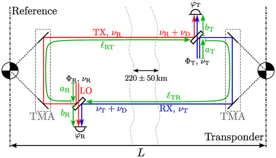
Figure 1. Simplified light paths and frequencies within the LRI. See the main text for an explanation.

On the reference side, the laser frequency ${\nu }_{\mathrm{R}}$ is stabilized by utilizing an optical reference cavity by using the PDH technique [11]. The residual frequency fluctuations $\delta {\nu }_{\mathrm{R}}$ were required to be below $30\mathrm{Hz}/\sqrt{\mathrm{Hz}}$ for Fourier frequencies above 10 $\mathrm{M}$Hz, with a relaxation towards lower Fourier frequencies [10,12]. The actual in-flight noise, expressed as amplitude spectral density (ASD), is well below the requirement and in the order of

$$\mathrm{ASD}\left[\delta {\nu }_{\mathrm{R}}\right]\left(f\right)\approx \frac{{10}^{-15}·{\nu }_{\mathrm{R}}}{\sqrt{\mathrm{Hz}}}\sqrt{\frac{f}{1\mathrm{Hz}}}\approx 0.3\frac{\mathrm{Hz}}{\sqrt{\mathrm{Hz}}}\sqrt{\frac{f}{1\mathrm{Hz}}}$$

(2)

at frequencies above 200 $\mathrm{M}$Hz [1], where it is dominant and directly apparent in the measured signal due to the lack of other signals at such high frequencies. Assessing the frequency stability at lower frequencies is difficult due to the dominant ranging signal arising from gravitational and non-gravitational differential forces acting on the satellites (cf. black trace in Figure 2, page 6).

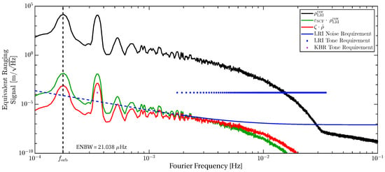
Figure 2. Typical amplitude spectral density of the LRI ranging signal (black) and effective errors arising from a static scale factor error ${\epsilon }_{\mathrm{SCF}}={10}^{-6}$ (green) and timeshift $\zeta =50 \mathsf{\mu }\mathrm{s}$ (red, cf. Equation (14)). Also shown is the noise requirement of the LRI (blue line), which is strictly applicable only for frequencies above 2 $\mathrm{M}$Hz, but it was extrapolated toward lower frequencies (blue dashed segment). The dots denote a 1 $\mathsf{\mu }$$\mathrm{m}$ tone amplitude, being the tone error requirement for KBR and LRI at specific frequencies (2/rev for KBR, 10/rev…200/rev for LRI). The ranging measurement is dominated by laser frequency noise at the highest frequencies (above 30 $\mathrm{M}$Hz), and by the differential gravitational and nongravitational forces below.

On the reference spacecraft, the laser light is split at the beamsplitter into a local oscillator (LO) part and into the transmit (TX) beam (cf. Figure 1). The Triple Mirror Assembly (TMA) routes the TX beam around cold-gas tanks (not shown) toward the distant spacecraft. The emitted frequency is Doppler-shifted when received on the transponder due to the relative motion of the two spacecraft. The relative velocity of the two spacecraft is below $\pm 2.5$ $\mathrm{m}$/$\mathrm{s}$, which translates into a one-way Doppler shift of ${\nu }_{\mathrm{D}}<\pm 2.5 \mathrm{MHz}$ [10].

The transponder unit employs a frequency-locked loop with a 10 $\mathrm{M}$Hz offset, meaning that the frequency ${\nu }_{\mathrm{T}}$ is controlled with high gain and bandwidth, such that the beatnote at the photodetector between the local and received, Doppler-shifted light stays at $f_{\mathrm{off}}=10 \mathrm{MHz}$. This enforces that the transponder laser frequency ${\nu }_{\mathrm{T}}$ is the sum of received Doppler-shifted reference frequency ${\nu }_{\mathrm{R}}^{\prime }={\nu }_{\mathrm{R}}+{\nu }_{\mathrm{D}}$ and $f_{\mathrm{off}}$. The transponder is to send back amplified laser light to the reference with a well-defined and known optical frequency (and phase). Because the transponder is in $220\pm 50$ $\mathrm{k}$$\mathrm{m}$ distance, it only receives a fraction of the initially emitted light power (on the order of nanowatts). The amplified and offset-locked beam travels back to the reference side, interferes again, and the beatnote between the (once more) Doppler-shifted transponder and local reference frequency $f_{\mathrm{R}}={\nu }_{\mathrm{T}}^{\prime }-{\nu }_{\mathrm{R}}=2{\nu }_{\mathrm{D}}+f_{\mathrm{off}}$ contains the desired ranging information, encoded in the Doppler shift ${\nu }_{\mathrm{D}}$.

3. Error Coupling in the Range Measurement

The previous section provided a descriptive picture of the LRI working principle through the beam’s frequencies. However, the LRI actually measures the differential phase of the two interfering light beams given by the time integral of the beatnote frequency. To describe the phase observables in a relativistic framework, we now follow the approach of Yan et al. [13] to assess potential relativistic effects on the scale factor. We favor this description in terms of phase because it is invariant in the context of general relativity, i.e., independent of the coordinate system, in contrast to the frequency.

The conversion of the measured differential phase

$${\phi }_{\mathrm{LRI}}={\phi }_{\mathrm{T}}-{\phi }_{\mathrm{R}}$$

(3)

to the range observable in a relativistic framework is given in [13,14] and is omitted here for brevity. The LRI range reads

$$\begin{array}{cc}\hfill {\rho }_{\mathrm{LRI}}^{\mathrm{raw}}\left(t\right)& =\frac{c_0}{2}{\int }_0^t\frac{\mathrm{d}{\phi }_{\mathrm{LRI}}\left(t^{\prime }\right)}{\mathrm{d}{t}^{\prime }}\frac{1}{{\nu }_{\mathrm{R}}^{\mathrm{G}}(t^{\prime }-\Delta t^{\left[\mathrm{rt}\right]}\left(t^{\prime }\right))}-\left(\frac{{\nu }_{\mathrm{R}}^{\mathrm{G}}\left(t^{\prime }\right)}{{\nu }_{\mathrm{R}}^{\mathrm{G}}(t^{\prime }-\Delta t^{\left[\mathrm{rt}\right]}\left(t^{\prime }\right))}-1\right)\mathrm{d}{t}^{\prime }\hfill \end{array}$$

(4)

$$\begin{array}{cc}\hfill & =\frac{c_0}{2}\left(\Delta t^{\left[\mathrm{rt}\right]}\left(t\right)-\Delta t^{\left[\mathrm{rt}\right]}\left(0\right)\right)+\mathrm{errors}.\hfill \end{array}$$

(5)

Equation (4) provides a recipe to compute the raw biased range as a function of the coordinate time t, which is available after precise orbit determination. The roundtrip propagation time is on the order of $\Delta t^{\left[\mathrm{rt}\right]}\approx 2·220 \mathrm{k}\mathrm{m}/c_0\approx 1.46 \mathrm{m}\mathrm{s}$ with the speed of light $c_0$ and the absolute laser frequency in the coordinate frame is given by ${\nu }_{\mathrm{R}}^{\mathrm{G}}$. The relation between the frequency of the laser source ${\nu }_{\mathrm{R}}$ and the apparent frequency in the Earth-centered geocentric celestial reference frame (GCRF) system ${\nu }_{\mathrm{R}}^{\mathrm{G}}$ is

$${\nu }_{\mathrm{R}}^{\mathrm{G}}={\nu }_{\mathrm{R}}·\frac{\mathrm{d}{\tau }_{\mathrm{R}}}{\mathrm{d}t},$$

(6)

where ${\tau }_{\mathrm{R}}$ is the proper time of the reference spacecraft and t is the coordinate time in the GCRF. The distinction between those is discussed in [14], and a neglection yields a tone error on the order of 1 $\mathsf{\mu }$$\mathrm{m}$ rms at 1/rev. The first term in the integral resembles the well-known relation

$$\rho \left(t\right)=\frac{c_0}{\nu }\phi \left(t\right),$$

(7)

and the second term accounts for the effect of a varying frequency ${\nu }_{\mathrm{R}}^{\mathrm{G}}\left(t\right)$.

Equation (5) in turn provides the physical meaning of ${\rho }_{\mathrm{LRI}}^{\mathrm{raw}}$ as a time-of-flight measurement, whereby the errors include tilt-to-length coupling [15], laser frequency noise [1], and others.

The representation until here is, however, neglecting some error sources. We now derive a model for two error sources, namely a mismodeling of the laser frequency, which can be expressed through a scale factor, and secondly from clock errors. Equation (4) shows that the intersatellite biased range can be reconstructed from phase measurements if the conversion factor, given by the absolute frequency ${\nu }_{\mathrm{R}}^{\mathrm{G}}\left(t\right)$ or wavelength $\lambda \left(t\right)=c_0/{\nu }_{\mathrm{R}}^{\mathrm{G}}\left(t\right)$, is known. If we consider errors in the knowledge of the frequency, given as the difference between estimated and true frequency ${\nu }_{\mathrm{R},\mathrm{est}}^{\mathrm{G}}\left(t\right)-{\nu }_{\mathrm{R}}^{\mathrm{G}}\left(t\right)$, this error is typically expressed as a scale factor

$${\epsilon }_{\mathrm{SCF}}\left(t\right)=\frac{{\nu }_{\mathrm{R},\mathrm{est}}^{\mathrm{G}}\left(t\right)-{\nu }_{\mathrm{R}}^{\mathrm{G}}\left(t\right)}{{\nu }_{\mathrm{R}}^{\mathrm{G}}\left(t\right)}\iff {\nu }_{\mathrm{R}}^{\mathrm{G}}\left(t\right)=\frac{{\nu }_{\mathrm{R},\mathrm{est}}^{\mathrm{G}}\left(t\right)}{1+{\epsilon }_{\mathrm{SCF}}\left(t\right)}.$$

(8)

By applying the replacement ${\nu }_{\mathrm{R}}^{\mathrm{G}}\left(t\right)\to {\nu }_{\mathrm{R}}^{\mathrm{G}}\left(t\right)/(1+{\epsilon }_{\mathrm{SCF}}\left(t\right))$ to Equation (4), we obtain an expression for the estimated range ${\rho }_{\mathrm{LRI}}^{\mathrm{raw},\mathrm{est}}$. In the following, we compute the error of this estimated range. For better readability, we drop the time dependency of terms evaluated at the measurement epoch $t^{\prime }$ in the integral. We have

$$\begin{array}{cc}\hfill & {\rho }_{\mathrm{LRI}}^{\mathrm{raw}},\mathrm{est}\left(t\right)-{\rho }_{\mathrm{LRI}}^{\mathrm{raw}}\left(t\right)\hfill \end{array}$$

$$\begin{array}{cc}\hfill & =\frac{c_0}{2}{\int }_0^t\frac{{\nu }_{\mathrm{R}}^{\mathrm{G}}+{\epsilon }_{\mathrm{SCF}}(t^{\prime }-\Delta t^{\left[\mathrm{rt}\right]})·{\dot{\phi }}_{\mathrm{LRI}}}{{\nu }_{\mathrm{R}}^{\mathrm{G}}(t^{\prime }-\Delta t^{\left[\mathrm{rt}\right]})}-\frac{(1+{\epsilon }_{\mathrm{SCF}}(t^{\prime }-\Delta t^{\left[\mathrm{rt}\right]})){\nu }_{\mathrm{R}}^{\mathrm{G}}}{(1+{\epsilon }_{\mathrm{SCF}}){\nu }_{\mathrm{R}}^{\mathrm{G}}(t^{\prime }-\Delta t^{\left[\mathrm{rt}\right]})}\mathrm{d}{t}^{\prime }\hfill \end{array}$$

(9)

$$\begin{array}{cc}\hfill & \approx \frac{c_0}{2}{\int }_0^t{\epsilon }_{\mathrm{SCF}}(t^{\prime }-\Delta t^{\left[\mathrm{rt}\right]})\Delta {\dot{t}}^{\left[\mathrm{rt}\right]}-{\epsilon }_{\mathrm{SCF}}(t^{\prime }-\Delta t^{\left[\mathrm{rt}\right]})+\frac{{\nu }_{\mathrm{R}}^{\mathrm{G}}{\epsilon }_{\mathrm{SCF}}}{{\nu }_{\mathrm{R}}^{\mathrm{G}}(t^{\prime }-\Delta t^{\left[\mathrm{rt}\right]})}\mathrm{d}{t}^{\prime }\hfill \end{array}$$

(10)

$$\begin{array}{cc}\hfill & \approx \frac{c_0}{2}{\int }_0^t{\epsilon }_{\mathrm{SCF}}\Delta {\dot{t}}^{\left[\mathrm{rt}\right]}+{\dot{\epsilon }}_{\mathrm{SCF}}\Delta t^{\left[\mathrm{rt}\right]}-{\epsilon }_{\mathrm{SCF}}+\frac{{\nu }_{\mathrm{R}}^{\mathrm{G}}{\epsilon }_{\mathrm{SCF}}}{{\nu }_{\mathrm{R}}^{\mathrm{G}}(t^{\prime }-\Delta t^{\left[\mathrm{rt}\right]})}\mathrm{d}{t}^{\prime }\hfill \end{array}$$

(11)

$$\begin{array}{cc}\hfill & \approx {\epsilon }_{\mathrm{SCF}}\left(t\right)·\frac{c_0}{2}\Delta t^{\left[\mathrm{rt}\right]}\left(t\right)+\frac{c_0}{2}{\int }_0^t{\epsilon }_{\mathrm{SCF}}\left(\frac{{\dot{\nu }}_{\mathrm{R}}^{\mathrm{G}}}{{\nu }_{\mathrm{R}}^{\mathrm{G}}}\Delta t^{\left[\mathrm{rt}\right]}+1\right)-{\epsilon }_{\mathrm{SCF}}\mathrm{d}{t}^{\prime }\hfill \end{array}$$

(12)

$$\begin{array}{cc}\hfill & \approx {\epsilon }_{\mathrm{SCF}}\left(t\right)·L\left(t\right),\hfill \end{array}$$

(13)

where we used some approximations justified below to obtain the simple result. The approximation in Equation (10) is based on the relation $1/(1+{\epsilon }_{\mathrm{SCF}})\approx 1-{\epsilon }_{\mathrm{SCF}}$ together with the definition of the phase derivative in ([14], Equation (27)) and we dropped a second-order term in ${\left({\epsilon }_{\mathrm{SCF}}\right)}^2$. Equation (11) uses ${\epsilon }_{\mathrm{SCF}}(t-\Delta t^{\left[\mathrm{rt}\right]})\approx {\epsilon }_{\mathrm{SCF}}\left(t\right)-\Delta t^{\left[\mathrm{rt}\right]}{\dot{\epsilon }}_{\mathrm{SCF}}\left(t\right)$ and neglects product terms of $\Delta t^{\left[\mathrm{rt}\right]}·\Delta {\dot{t}}^{\left[\mathrm{rt}\right]}$. The result of Equation (12) employed the same type of approximations, namely $1/{\nu }_{\mathrm{R}}^{\mathrm{G}}(t^{\prime }-\Delta t^{\left[\mathrm{rt}\right]})\approx (1+{\dot{\nu }}_{\mathrm{R}}^{\mathrm{G}}/{\nu }_{\mathrm{R}}^{\mathrm{G}}·\Delta t^{\left[\mathrm{rt}\right]})/{\nu }_{\mathrm{R}}^{\mathrm{G}}$. To solve the integral, we omitted product terms of ${\dot{\nu }}_{\mathrm{R}}^{\mathrm{G}}/{\nu }_{\mathrm{R}}^{\mathrm{G}}$ with ${\epsilon }_{\mathrm{SCF}}$ or ${\dot{\epsilon }}_{\mathrm{SCF}}$, because these describe a second-order cross-coupling between scale error and fractional true frequency change that is expected to be negligible. $L\left(t\right)=c_0\Delta t^{\left[\mathrm{rt}\right]}\left(t\right)/2$ denotes the absolute distance between the spacecraft and the error coupling ${\epsilon }_{\mathrm{SCF}}\left(t\right)·L\left(t\right)$ resembles the well-known influence of (fractional) laser frequency variations into the range measurement [10], which can be regarded as a scale factor error.

The second error contributor that we address is a potential timeshift $\zeta$ of the measured LRI data, arising from unmodeled internal delays of the LRI. At startup, the LRI time is initialized via the Onboard Computer (OBC), which introduces a delay of $1.5$ $\mathrm{s}$ at maximum [16], although we only observed values below $1.0$ $\mathrm{s}$. To compensate for this delay, the differences of LRI time and MWI Instrument Processing Unit (IPU) time are measured regularly (called the datation report) and are used to correct the LRI time tags. However, a small deviation $\zeta$ may remain, even after this subtraction. We linearize the effect of this potential timeshift to first order as

$${\rho }_{\mathrm{LRI}}^{\mathrm{inst}}(t+\zeta )\approx {\rho }_{\mathrm{LRI}}^{\mathrm{inst}}\left(t\right)+\zeta ·\dot{\rho }\left(t\right),$$

(14)

where we use the approximate range rate $\dot{\rho }\approx {\dot{\rho }}_{\mathrm{LRI}}^{\mathrm{raw}}\approx {\dot{\rho }}_{\mathrm{LRI}}^{\mathrm{inst}}$ for terms that describe a small error coupling and where the highest precision in $\dot{\rho }$ is not required.

Figure 2 illustrates the significance of the static scale factor error ${\epsilon }_{\mathrm{SCF}}={10}^{-6}$ (green) and timeshift $\zeta =50 \mathsf{\mu }\mathrm{s}$ (red), which represent the common orders of magnitude in current LRI data processing. The effects of these exceed or are close to the LRI noise requirement for frequencies between $0.6\dots 3 \mathrm{MHz}$, indicating that the scale factor and timeshift need to be known to better precision, e.g., at the level of 10⁻⁷ to 10⁻⁸ for the scale and at a level of a few microseconds or better for the timeshift. Fourier frequencies below $0.6 \mathrm{MHz}$ are dominated by sinusoidal errors at integer multiples of the orbital frequency $f_{\mathrm{orb}}\approx 0.18 \mathrm{MHz}$. These peaks need to be compared to tone error requirements with the unit of a meter (rms or peak) instead of spectral densities with the unit of $\mathrm{m}/\sqrt{\mathrm{Hz}}$. The GRACE-FO tone error requirement is 1 $\mathsf{\mu }$$\mathrm{m}$_peak [9], applying to the MWI at 2/rev frequency and to the LRI for $n/\mathrm{rev}$ frequencies with $10\le n\le 200$. The tone requirement can be compared to the traces in Figure 2 (see blue dots), if the 1 $\mathsf{\mu }$$\mathrm{m}$ tone value is rescaled to a level of $1 \mathsf{\mu }{\mathrm{m}}_{\mathrm{peak}}/\sqrt{2\mathrm{ENBW}}\approx$ 1.5 × 10⁻⁴ $\mathrm{m}/\sqrt{\mathrm{Hz}}$ [17] by using the equivalent noise bandwidth (ENBW) of $\approx 21 \mathsf{\mu }\mathrm{Hz}$ that was used to compute the spectral density traces. The LRI tone error is not specified at lower frequencies ($n<10$), as the instrument is only a technology demonstrator, but in future missions the LRI may inherit the 2/rev requirement from the MWI, justifying the appearence of the MWI requirement in Figure 2. The displayed errors (green and red) exceed the one-micron tone level by approximately two orders of magnitude at 1/rev and 2/rev frequencies.

By combining the effects due to a scale factor error (Equation (13)) and an uncompensated timeshift (Equation (14)), we obtain the error of the LRI measured range with regard to the truth as

$${\rho }_{\mathrm{LRI}}^{\mathrm{inst}}\left(t\right)-{\rho }_{\mathrm{true}}^{\mathrm{inst}}\left(t\right)\approx {\epsilon }_{\mathrm{SCF}}\left(t\right)·L\left(t\right)+\zeta ·\dot{\rho }\left(t\right).$$

(15)

4. Scale Factor Determination

The scale factor ${\epsilon }_{\mathrm{SCF}}$ implicitly defined in Equation (1) provides an estimate ${\nu }_{\mathrm{R},\mathrm{est}}$ for the actual laser frequency ${\nu }_{\mathrm{R}}$ of the LRI reference unit, which in turn is needed for accurately converting the phase measurement into a range in meter. Here we present three approaches to either directly calculate the absolute laser frequency ${\nu }_{\mathrm{R}}$ or through the scale factor ${\epsilon }_{\mathrm{SCF}}$ that is related to absolute laser frequency through Equation (8).

Because GRACE-FO hosts the KBR and LRI, which are designed to measure the same quantity in parallel, the obvious way to obtain the LRI scale ${\epsilon }_{\mathrm{SCF}}$ (or frequency ${\nu }_{\mathrm{R}}$) is to compare the ranging data of the two instruments. We define the instantaneous KBR range as

$${\rho }_{\mathrm{KBR}}^{\mathrm{inst}}\left(t\right)={\rho }_{\mathrm{KBR}}^{\mathrm{raw}}\left(t\right)+{\rho }_{\mathrm{KBR}}^{\mathrm{LTC}}\left(t\right)+{\rho }_{\mathrm{KBR}}^{\mathrm{AOC}}\left(t\right).$$

(16)

The three quantities on the right-hand side are the ionosphere-free K/Ka-band range ${\rho }_{\mathrm{KBR}}^{\mathrm{raw}}$, the KBR Light Time Correction (LTC) and the antenna offset correction (AOC), which are regarded as error-free here. They are given in the KBR1B data product [16]. Ultimately, daily arcs of LRI phase measurements can be calibrated against the KBR ranging data, i.e., by minimizing the KBR-LRI residuals as

$$∥{\rho }_{\mathrm{KBR}}^{\mathrm{inst}}\left(t\right)-{\lambda }_{\mathrm{est}}^{\mathrm{SDS}}·{\phi }_{\mathrm{LRI}}(t+\zeta )-{\rho }_{\mathrm{LRI}}^{\mathrm{LTC}}∥\to 0$$

(17)

by using a daily constant laser wavelength ${\lambda }_{\mathrm{est}}^{\mathrm{SDS}}$ and timeshift $\zeta$ as fit parameters. The KBR scale factor error can be regarded as negligible because the relevant Ultra-Stable Oscillator (USO) frequency is determined during precise orbit determination by referencing it to global positioning system (GPS). The USO fractional frequency varies by about 10⁻¹¹, mainly at 1/rev ([14], Figure 1), and we assume the knowledge error to be even smaller. The processing of daily chunks of data essentially decomposes the scale factor ${\epsilon }_{\mathrm{SCF}}$ into a static and time-variable part as

$${\epsilon }_{\mathrm{SCF}}\left(t\right)=⟨{\epsilon }_{\mathrm{SCF}}⟩+\delta {\epsilon }_{\mathrm{SCF}}\left(t\right),$$

(18)

of which only the static part $⟨{\epsilon }_{\mathrm{SCF}}⟩$ is determined separately on every day with discontinuities at the day boundary.

This cross-calibration scheme is the official processing strategy employed by the Science Data System (SDS) for the LRI1B data product in version 04, wherein a conversion factor from phase to range and a timeshift $\zeta$ is estimated once per day. The scale $⟨{\epsilon }_{\mathrm{SCF}}^{\mathrm{SDS}}⟩$ is reported in the ionospheric correction (iono_corr) column of the LRI1B files, whereas the timeshift $\zeta$ is applied through LLK1B. The scale value relates to the laser frequency and wavelength estimates of the reference laser through

$$\begin{array}{cc}\hfill & {\lambda }_{\mathrm{est}}^{\mathrm{SDS}}\left(t_{\mathrm{daily}}\right)=(1+⟨{\epsilon }_{\mathrm{SCF}}^{\mathrm{SDS}}⟩\left(t_{\mathrm{daily}}\right))·{\lambda }_0\hfill \end{array}$$

(19)

and

$$\begin{array}{cc}\hfill & {\nu }_{\mathrm{est}}^{\mathrm{SDS}}\left(t_{\mathrm{daily}}\right)=\frac{{\nu }_0}{\left(1+⟨{\epsilon }_{\mathrm{SCF}}^{\mathrm{SDS}}⟩\left(t_{\mathrm{daily}}\right)\right)},\hfill \end{array}$$

(20)

where ${\nu }_0$ is a nominal frequency for the LRI lasers, given in the documentation as ${\nu }_0$ = 281,616,393 $\mathrm{M}$Hz and ${\nu }_0$ = 281,615,684 $\mathrm{M}$Hz for GF-1 and GF-2, respectively [16]. The two nominal values were determined preflight, but do not represent the best knowledge of the actual frequency. The corresponding nominal wavelength is ${\lambda }_0=c_0/{\nu }_0$. Equation (20) is in principle a reformulation of Equations (8 )and (18), however, the time-varying part $\delta {\epsilon }_{\mathrm{SCF}}\left(t\right)$ is neglected by the processing of daily segments. Therefore, Equation (4) simplifies to

$${\rho }_{\mathrm{LRI}}^{\mathrm{SDS}}\left(t\right)=\frac{c_0}{2}\frac{(1+⟨{\epsilon }_{\mathrm{SCF}}^{\mathrm{SDS}}⟩)}{{\nu }_0}·{\phi }_{\mathrm{LRI}}\left(t\right).$$

(21)

The minimization result for $⟨{\epsilon }_{\mathrm{SCF}}^{\mathrm{SDS}}⟩$, as given in the LRI1B-v04 data product, is shown in green in Figure 3. Our recomputation with an in-house Level 1A to 1B processing is denoted as $⟨{\epsilon }_{\mathrm{SCF}}^{\mathrm{AEI}}⟩$ (blue), which will be used later on as one possible frequency model. The plot covers the timespan from 13 December 2018 until 1 January 2022, where GF-1 acts as the LRI reference unit. Due to spacecraft-related outages, the LRI was not in science mode from 6 February 2019 to 17 March 2019. Smaller gaps in the data originate from phase breaks, e.g., due to spacecraft maneuvers or diagnostic data recording. The frequent data gaps starting in mid-2021 are due to nadir-pointing of the spacecraft, occurring roughly two days per week. In these periods, the pointing angles between the spacecraft-fixed coordinate system and the line-of-sight exceed the LRI pointing capabilities.

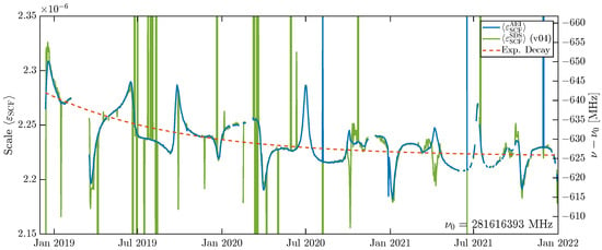
Figure 3. Comparison of LRI scale factor $⟨{\epsilon }_{\mathrm{SCF}}⟩$ using the conventional cross-calibration method. Blue: using the AEI ranging phase ${\phi }_{\mathrm{LRI}}$, cf. Equation (4). Green: the SDS LRI1B-v04 result. Orange dashed: Exponential model for the cavity resonance frequency.

Even though the blue and green traces roughly match, the SDS implementation seems less robust as it shows more outliers, which may be related to imperfect phase jump removal [1]. The number of outliers reduced after 27 June 2020, when the deglitching algorithm was adjusted by the SDS [18]. Both traces show a slow drift that seems to converge and peaks and dips occurring roughly every three months, indicating an apparent change of the laser frequency with a magnitude of ±10⁻⁷ or $\pm 20$ $\mathrm{M}$Hz. It is noteworthy that we cannot distinguish which instrument contributes to those periodic variations, as we always use the difference between LRI and KBR. However, Section 8 and Section 9 will address these variations in more detail. The slow drift in Figure 3 was fitted as exponential decay of the form

$${\epsilon }^{\mathrm{Cav}}\left(t\right)={\epsilon }_{\infty }^{\mathrm{Cav}}-{\epsilon }_0^{\mathrm{Cav}}exp(-{\lambda }^{\mathrm{Cav}}·t)$$

(22)

and is shown in orange. The decay rate is ${\lambda }^{\mathrm{Cav}}=$4.006 × 10⁻⁸$/\mathrm{s}$, with ${\epsilon }_{\infty }^{\mathrm{Cav}}=$2.221 × 10⁻⁶ and ${\epsilon }_0^{\mathrm{Cav}}=$−1.190 × 10⁻⁷, the time t is GPS seconds past 22 May 2018, 00:00:00 UTC. Exponential shrinkage (and thus increasing frequency) has already been observed in similar cavities made from ultra-low expansion (ULE) materials, and the suspected cause is aging of the spacer material [19]. Equation (22) can of course be converted into an equivalent frequency model ${\nu }_{\mathrm{R}}^{\mathrm{Cav}}$ via Equation (20). This exponential model is the second model for the laser frequency, resulting in similar values as the SDS scheme, but without the periodic features. Until now, we only derived these exponential model coefficients for GF-1. The derivation for GF-2 is beyond the scope of this manuscript as GF-2 was only for short times in reference mode.

The scheme of cross-calibration is only possible due to the unique situation of having two independent ranging measurements by KBR and LRI. However, it cannot resolve intraday frequency variations of the LRI and introduces small discontinuities at day bounds. Furthermore, it depends on the KBR, which will likely not be present in future missions. Therefore we present an on-ground calibration that has been performed for the two laser flight models as a third method by which to determine the laser frequency and derive a calibrated frequency model by only using telemetry data of the LRI. It is based on the fact that the laser frequency ${\nu }_{\mathrm{R}}$ can be deduced from the setpoints of the laser’s frequency-lock control loop and thermal state. With this model, we can continuously evaluate the optical frequency in orbit with moderate accuracy. The laser frequency may change due to varying environmental conditions, e.g., temperatures of the optical reference cavity. This model will be derived in Section 5, Section 6 and Section 7, and all models are analyzed and compared to each other in Section 8.

5. LRI Laser and Telemetry Description

The LRI Reference Laser Units (RLUs) were built by Tesat Spacecom and are comparable to the laser onboard LISA Pathfinder and to the seed laser of one possible LISA implementation [20]. They are based on an Nd:YAG non-planar ring oscillator (NPRO) crystal and are fiber-connected to an optical reference cavity built by Ball Aerospace [12,21] and to the Optical Bench Assembly (OBA). The laser’s output power is in the order of 25 $\mathrm{m}$$\mathrm{W}$ in the near-infrared regime ($\lambda \approx 1064 \mathrm{n}\mathrm{m}$) [22]. The laser frequency is actively controlled by feedback control loops either from the reference cavity by using the PDH scheme [11] (in reference mode) or to the incoming beam by using a frequency-offset lock (transponder mode). The tuning is achieved through a thermal element for slow variations and a Piezo-Electric Transducer (PZT) actuator for fast variations. The actuator signals are downlinked in the laser telemetry and published within the LHK1A/B data products at a rate of 1 Hz, if the LRI is in science mode, i.e., when the laser link is established. The data type is unsigned integer of 32-bit depth. The corresponding normalized signed data streams are computed via the two’s complement and scaling by the bit depth as

$$\mathtt{u}\mathtt{2}\mathtt{i}(x,N)=\{\begin{array}{cc}x/2^N-1,& \mathrm{if}x\ge 2^{N-1}\hfill \\ x/2^N,& \mathrm{if}x<2^{N-1}\hfill \end{array}$$

(23)

with $N=32$ and x denoting the unsigned value from the telemetry. The value range is $-1/2<\mathtt{u}\mathtt{2}\mathtt{i}(x,·)\le 1/2$. In the following, these normalized data streams are denoted as pztIL, pztOOL, thermIL and thermOOL. The temperature of the laser can be retrieved from so-called “OFFRED” data, which is recorded by the OBC. The measurement is taken at the Thermal Reference Point (TRP) of the RLU, which is located at the laser’s housing. By the time of writing, the laser TRP temperature is not publicly available. Still, it will be shown later that the influence of the TRP coupling is small during nominal operations.

The notations in-loop (IL) and out-of-loop (OOL) are not referring to different sensors as in conventional feedback control circuits, but two parts that are added to form the final setpoint. The OOL channel is used for manual control with some logic (e.g., to drive a frequency ramp for locking to the cavity or during acquisition). In contrast, the IL value represents the evolution of the actuator value in closed-loop operation. The actuator range of the PZT and thermal actuators is $\pm 1$ $\mathrm{V}$ and $\pm 9$ $\mathrm{V}$, respectively, with nominal frequency coupling coefficients of 5 $\mathrm{M}$Hz/$\mathrm{V}$ and 500 $\mathrm{M}$Hz/$\mathrm{V}$, respectively, also shown in Table 1.

Table 1. Coupling factors for the two LRI laser flight units. Shown are the design values provided by the laser manufacturer and fit results from on-ground measurements. PZT and TRP coupling factors were not refined, because the measurements were not suitable to derive these couplings. The static value $\Delta {\nu }_{\mathrm{AirToVac}}$ was provided by the manufacturer and represents the frequency change from air to vacuum. The shown uncertainties are the formal errors of the least squares estimation.

Coupling	Unit	Design Value	GF-1 (Fit)	GF-2 (Fit)
$c_{\mathtt{pztIL}}$	[MHz]	$2 \mathrm{V}·5 \mathrm{MHz}/\mathrm{V}=10 \mathrm{MHz}$	-	-
$c_{\mathtt{pztOOL}}$	[MHz]	$18 \mathrm{V}·5 \mathrm{MHz}/\mathrm{V}=90 \mathrm{MHz}$	-	-
$c_{\mathtt{thermIL}}$	[MHz]	$2 \mathrm{V}·500 \mathrm{MHz}/\mathrm{V}=1000 \mathrm{MHz}$	$1097\pm 0.383$	$1094\pm 1.383$
$c_{\mathtt{thermOOL}}$	[MHz]	$18 \mathrm{V}·500 \mathrm{MHz}/\mathrm{V}=9000 \mathrm{MHz}$	$9155\pm 7.396$	$8857\pm 27.565$
$c_{\mathtt{lasTRP}}$	[MHz/K]	−12	-	-
${\nu }_{0,\mathrm{air}}$	[MHz]	281,614,803 (GF-1) 281,614,780 (GF-2)	$\mathrm{281,614,682.081}$ $\pm 0.378$	$\mathrm{281,614,631.999}$ $\pm 1.094$
$\Delta {\nu }_{\mathrm{AirToVac}}$	[MHz]	37 (GF-1) 27 (GF-2)	-	-

6. RLU On-Ground Calibration

The laboratory setup used to calibrate the LRI lasers is shown in Figure 4. It consisted of the LRI flight laser, the Laser Ranging Processor (LRP) (including the phasemeter), a frequency-controlled reference laser and a wavemeter. The measurements were performed by parts of the LRI teams at JPL/NASA and AEI Hannover.

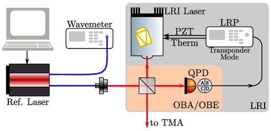
Figure 4. Laboratory setup for the LRI flight laser frequency calibration measurement. Blue lines denote optical fibers; red lines are laser beams in free space. Black arrows denote electric signals.

During these activities, the frequency of the reference laser was tuned by using a computer, and its frequency was recorded by using a wavemeter. The LRI unit in transponder mode locks its laser frequency to the incoming beam and adds a 10 $\mathrm{M}$Hz offset and is thus known as well. During the activities, the RLU temperature, as well as the PZT and thermal telemetry, is recorded. The frequency of the LRI laser was not measured directly, because it was more convenient to use the second output port of the reference laser (one fiber to the wavemeter, one to the optical bench), whereas the LRI laser light is free-beam on the optical bench. We use a linear model to estimate the laser frequency based on the telemetry (TM):

$${\nu }^{\mathrm{TM}}\left(t\right)=\left(\begin{array}{c}{c}_{\mathtt{pztIL}}\\ c_{\mathtt{pztOOL}}\\ c_{\mathtt{thermIL}}\\ c_{\mathtt{thermOOL}}\\ c_{\mathtt{lasTRP}}\end{array}\right)·\left(\begin{array}{c}\mathtt{pztIL}\left(t\right)\\ \mathtt{pztOOL}\left(t\right)\\ \mathtt{thermIL}\left(t\right)\\ \mathtt{thermOOL}\left(t\right)\\ \mathtt{lasTRP}(t-\tau )-26°\mathrm{C}\end{array}\right)+{\nu }_{0,\mathrm{air}}+\Delta {\nu }_{\mathrm{AirToVac}},$$

(24)

which depends on the actuator states, i.e., the telemetry data streams pztIL, pztOOL, thermIL, thermOOL as well as the surrounding temperature, which is measured at the TRP of the laser. Because the TRP is located outside the thermal shielding, a time delay of $\tau =520 \mathrm{s}$ is applied to the temperature measurements, which represents the propagation time of outer temperature changes to the NPRO crystal. The manufacturer provided this numerical value. Furthermore, only deviations from the nominal temperature of 26 °C are considered.

The nominal values for the coupling factors given by the laser manufacturer are shown in Table 1. However, we refine the individual laser units’ thermal coupling coefficients with our measurements. The PZT and TRP coupling are not refined because they were not modulated strongly enough during the calibration measurements to derive reliable coupling factors. We expect the TRP coupling to be noncritical because the lasers’ TRP temperature varies only in the sub-Kelvin domain in flight as shown in Figure 5. The blue trace depicts the daily averaged laser TRP recording of GF-1 and its respective daily minimum (green) and maximum (red) values.

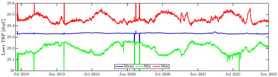
Figure 5. Daily mean, min, and max of the GF-1 lasTRP data.

The temperature of the GF-1 laser is stable when averaged daily. It shows subdaily variations of $\pm 0.2 \mathrm{K}$, which translates into $\Delta \nu =\pm 2.4 \mathrm{MHz}$ in frequency, or ${\epsilon }_{\mathrm{SCF}}\approx \Delta \nu /\nu \approx \pm 8.5\times {10}^{-9}$ by using a coupling of $-12$ $\mathrm{M}$Hz/$\mathrm{K}$ (cf. Table 1).

Several calibration measurements were performed on both RLUs between July 2017 and January 2018. For the laser integrated into GF-2, four measurements were taken. In the following, we label these four measurements (1)…(4). They all differ a little in their procedure. In (1), the reference laser’s frequency was commanded in discrete steps, which caused the LRP to lose lock and forced reacquisition and thus a temporary data loss. Afterward, the reference laser was put into a free-running cool-down mode without active stabilization. Reacquisition was avoided in (2) by sweeping continuously over the same frequency range. In (3) a diagnostic test was used for the Differential Wavefront Sensing (DWS), and the absolute frequency measurement was a secondary result. Test (4) consists of very few sample points only because the used wavemeter had no digital output port but only a display to retrieve the data. Thus, this analysis does not use the data of (4). The measurements (1) and (2) were performed in July 2017 by using a HighFinesse WS7-60 wavemeter with an absolute accuracy of 60 $\mathrm{M}$Hz. Test (3) in November 2017 used a HighFinesse WS6-600 (600 $\mathrm{M}$Hz accuracy) and in (4), a Burleigh WA1500 (60 $\mathrm{M}$Hz accuracy) was used. The GF-1 laser was tested twice—once with a WS6-600 in November 2017 and a Burleigh WA1500 in January 2018, and again, the latter one is not used in this analysis.

We use a least-squares approach to estimate the linear coupling factors and constants of Equation (24). Additionally, we weigh the WS7-60 measurements higher by a factor of 5 compared to the WS6-600, which has lower accuracy. We furthermore estimate a relative offset of the WS6-600 wavemeter, which we can deduce by analyzing the residuals. This offset of the WS6-600 is also apparent when measuring an absolute frequency reference like an iodine cell; see Appendices Appendix A and Appendix B for more information.

Figure 6 shows the regression result using the measurements for GF-2.

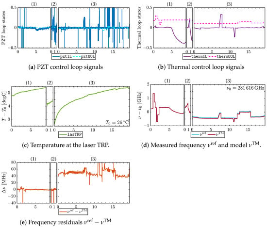
Figure 6. Regression results for the GF-2 laser. The numbering on top of the individual panels of each subfigure corresponds to the measurement campaigns, as explained in the text. Note the offset in the residuals in (e) when the less precise wavemeter WS6-600 was used in campaign (3). The average bias here is $51.494\pm 0.24$ $\mathrm{M}$Hz. All x-axes are in arbitrary time units.

The individual measurement campaigns are labeled (1)…(3). The subfigures (a) and (b) show the normalized telemetry of the laser control loops, and the temperature of the laser’s TRP is shown in subfigure (c). Panel (d) contains the absolute frequency of the reference laser ${\nu }^{\mathrm{ref}}$ (shifted by 10 $\mathrm{M}$Hz to compensate for the offset-frequency lock of the LRP) and the resulting laser frequency model ${\nu }^{\mathrm{TM}}$ of the LRI laser. The trace in (e) shows the residuals ${\nu }^{\mathrm{ref}}-{\nu }^{\mathrm{TM}}$, which clearly exhibits an offset of approximately 50 $\mathrm{M}$Hz beginning at (3), where the WS6-600 was used. The high-frequency variations are higher in (3) due to the lower precision of the WS6-600. The resulting coupling factors from the linear least squares minimization are shown in Table 1. Generally, the resulting values match the manufacturer’s design values with only slight deviations.

7. Empirical Refinement of Telemetry-Based Laser Frequency Model

The calibrated telemetry models ${\nu }_{1/2}^{\mathrm{TM}}$ are now compared to the frequency ${\nu }_{\mathrm{est}}^{\mathrm{SDS}}$ (cf. Equation (20)) from the KBR-LRI cross-correlation, where the flight data spanning from 13 December 2018 until 1 January 2022 is used. Figure 7 shows the frequency estimates from the TM models for both spacecraft (blue and yellow) alongside the SDS frequency (green). The latter is already shown in Figure 3, but outliers were removed this time. The GF-2 curves are shifted down by 10 $\mathrm{M}$Hz to remove the intended transponder frequency offset (cf. Section 2). The subscript $1/2$ refers to GF-1 or GF-2, respectively.

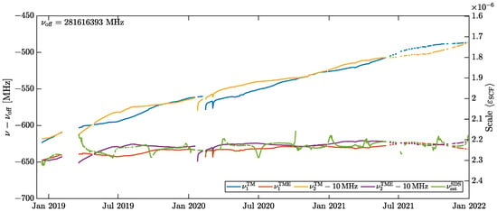
Figure 7. Purely ground calibration-based models ${\nu }_{1/2}^{\mathrm{TM}}$ and empirically corrected TM models ${\nu }_{1/2}^{\mathrm{TME}}$ for GF-1 and GF-2 laser frequencies alongside the SDS frequency ${\nu }_{\mathrm{est}}^{\mathrm{SDS}}$ from KBR-LRI cross-calibration. Outliers in SDS curve removed. The right axis shows approximate equivalent laser frequency variations, cf. Equation (20).

The models (blue and yellow) differ by 20 $\mathrm{M}$Hz at maximum, which is within the accuracy of the better wavemeter WS7-60, defining the model accuracy. However, a drift of the models w. r. t. the KBR cross-calibration method (green) is visible. The current hypothesis to explain this drift is an aging effect of the NPRO crystal or the electronics within the LRP. However, there is little literature on aging-induced frequency changes of NPRO lasers, and this theory might need verification in a laboratory experiment. The drift appears only in the laser setpoint telemetry but not in the frequency, which is tightly locked to the cavity resonance.

The curves show some data gaps starting in mid-2021, caused by regular nadir-pointing periods, in which the LRI was not creating science data. The steep slopes and the dip in February and March 2020 in ${\nu }_{1/2}^{\mathrm{TM}}$ are due to spacecraft-related nonscience phases of the LRI, after which the units had to heat up to reach the nominal temperatures. This heating process is visible at the laser TRP (cf. Figure 5) and thus affects not only the TM model but also the green SDS curve with comparable magnitude, which confirms the temperature coupling estimate in the TM model. However, we found that the link acquisition happened before the lasers reached their thermal equilibrium, which led to an apparent small step in the ${\nu }_{1/2}^{\mathrm{TM}}$ frequency model (see Appendix C). Imperfect coupling factors could possibly cause this. To account for these steps ${\nu }_i^{\mathrm{step}}$ in our telemetry-based laser frequency model, as well as for the drifts a and offsets $\Delta \nu$ from the NPRO aging, we define an empirical correction and estimate its parameters by least-squares minimization by using ${\nu }_{\mathrm{est}}^{\mathrm{SDS}}$ as the reference. The empirical model reads

$${\nu }^{\mathrm{emp}}\left(t\right)=a·(t-t_0)+\Delta \nu +{\nu }^{\mathrm{step}}\left(t\right),$$

(25)

where the reference epoch $t_0=\mathrm{1,210,982,400}$ GPS is 2018-May-22 at midnight. The steps are defined as

$$\begin{array}{c}\hfill {\nu }^{\mathrm{step}}\left(t\right)={\nu }_i^{\mathrm{step}}\mathrm{if}{t}_i^{\mathrm{step}}\le t<t_{i+1}^{\mathrm{step}}.\end{array}$$

(26)

The estimated parameters a and $\Delta \nu$ are shown in Table 2a, whereas the steps ${\nu }_i^{\mathrm{step}}$ and the corresponding time-tags $t_i^{\mathrm{step}}$ are shown in Table 2b. Unfortunately, this empirical model makes the telemetry-based frequency model still dependent on the KBR. In principle, one could overcome the needs of an empirical model by better calibrating the laser before launch.

Table 2. Parameters for the empirical part of the laser frequency model for GF-1 and GF-2 of Equation (25). Time tags refer to midnight.

(a) Drift Parameters				(b) Steps in the Telemetry-Based Laser Frequency Model
Coupling	Unit	Value		$\mathit{i}$	${\mathit{t}}_{\mathit{i}}^{\mathbf{step}}$	${\mathit{\nu }}_{\mathit{i}}^{\mathbf{step}}$[MHz]
		GF-1	GF-2			GF-1	GF-2
a	[$\mathrm{Hz}/\mathrm{s}$]	1.419	1.110	1	22 May 2018	0	0
$\Delta \nu$	[$\mathrm{M}\mathrm{Hz}$]	−5.881	−1.089	2	10 January 2020	0	−1.770
				3	10 February 2020	−11.593	2.881
				4	11 May 2020	−10.446	2.881
				5	1 January 2022	undefined	undefined

This empirical model is subtracted from the telemetry model to form the final telemetry-based and empirically corrected TME frequency estimate

$${\nu }_{1/2}^{\mathrm{TME}}\left(t\right)={\nu }_{1/2}^{\mathrm{TM}}\left(t\right)-{\nu }_{1/2}^{\mathrm{emp}}\left(t\right).$$

(27)

After applying the empirical model, the numerical values of the total frequency models ${\nu }_{1/2}^{\mathrm{TME}}$ for GF-1 and GF-2 (orange and purple traces in Figure 7) are in the range of ${\nu }_{\mathrm{est}}^{\mathrm{SDS}}$. In addition to the cross-calibration method, the telemetry-based model does not show seasonal or periodic features. Note that the exponential drift of the cavity is contained in ${\nu }_{\mathrm{est}}^{\mathrm{SDS}}$ and ${\nu }_{1/2}^{\mathrm{TME}}$, even though it is hard to see in the Figure 7. However, the empirical model in Equation (25) does not absorb the effect of exponentially increasing frequency (cf. Figure 3 and Equation (22)), because that cavity drift is present in both, ${\nu }_1^{\mathrm{TME}}$ and the reference ${\nu }_{\mathrm{est}}^{\mathrm{SDS}}$; thus, it is not apparent in the metric of the least-squares adjustment.

8. Comparison of the LRI1B-Equivalent Datasets

We define the prefit range error based on the instantaneous range difference between the LRI and KBR,

$${\rho }_{\mathrm{err},\mathrm{v}5\mathrm{X}}^{\mathrm{pre}}\left(t\right)={\rho }_{\mathrm{LRI},\mathrm{v}5\mathrm{X}}^{\mathrm{inst}}\left(t\right)-{\rho }_{\mathrm{KBR}}^{\mathrm{inst}}\left(t\right)-{\rho }_{\mathrm{KBR}}^{\mathrm{FV}}\left(t\right).$$

(28)

The subscript v5X denotes three different versions of the LRI1B data product derived at the Albert-Einstein Institute (AEI) [14,23]. They differ by the models for the laser frequency ${\nu }_{\mathrm{R}}^{\mathrm{G}}$. At first, the data product using the telemetry-based model described in the previous section (cf. Equation (27)) is called LRI1B-v51. The exponential cavity model (cf. Equation (22)) forms LRI1B-v52. The last data product, LRI1B-v53, uses the predetermined, constant value ${\nu }_0$ only, which makes it, in principle, a prerelease of LRI1B-v04 without the daily scale $⟨{\epsilon }_{\mathrm{SCF}}^{\mathrm{SDS}}⟩$, and timeshift $\zeta$ applied. The other differences between all three versions and the official v04 data are the improved deglitching algorithm [23] and the LTC implementation according to Yan et al. [13]. The LRI ranging data for these three versions at a 10 Hz data rate is derived for the time spanning from 13 December 2018 until 1 January 2022. We further used a correction ${\rho }_{\mathrm{KBR}}^{\mathrm{FV}}$ for the intraday carrier frequency variations of the KBR. This correction mainly contains signal at 1/rev and 2/rev frequency [14] and improves the consistency between SDS-derived KBR and AEI-derived LRI data products, because the AEI-derived LRI products include such a correction arising from the difference between proper time and coordinate GPS time (cf. ${\nu }_{\mathrm{R}}\left(t\right)$ vs. ${\nu }_{\mathrm{R}}^{\mathrm{G}}\left(t\right)$ in Section 3). However, the magnitude of this effect is small, and the results barely change when the correction is omitted.

In general, the range error exhibits long-term drifts in the order of a few 10 $\mathsf{\mu }$$\mathrm{m}$/day, which we remove through a high-pass Finite Impulse Response (FIR) filter with a cutoff frequency of $0.08 \mathrm{MHz}\approx f_{\mathrm{orb}}/2$. Future studies may address the reason for these long-term drifts, but this is beyond the scope of this article at the current stage. As mentioned in Section 4, the LRI scale factor is sensitive to variations or errors at 1/rev and 2/rev frequencies, which are unaffected by the filter. Due to the filtering, half a day of data is cropped at the start and end of each continuous segment, i.e., at every loss of the interferometric link of either KBR or LRI, to remove the initialization of the FIR filter. Hence, all gaps appear longer than they actually are. In the following, filtered quantities are denoted with a tilde, e.g.,

$${\tilde{\rho }}_{\mathrm{err},\mathrm{v}5\mathrm{X}}^{\mathrm{pre}}\left(t\right)=\mathrm{HPF}({\rho }_{\mathrm{err},\mathrm{v}5\mathrm{X}}^{\mathrm{pre}},0.08 \mathrm{MHz}).$$

(29)

The filtered prefit range errors for the three different LRI data products (v51, v52, v53) are shown as blue traces in Figure 8. For saving computational costs, the range error is decimated to a sampling rate of $3.3$ $\mathrm{M}$Hz.

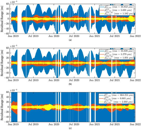
Figure 8. Prefit range error (Equation (29), blue) and postfit range error before (Equation (30), orange) and after (Equation (32), yellow) TC fitting for all three frequency models. Initially, the prefit KBR-LRI range error shows rms variations of 25 $\mathsf{\mu }$$\mathrm{m}$, 25 $\mathsf{\mu }$$\mathrm{m}$, 664 $\mathsf{\mu }$$\mathrm{m}$ for v51, v52 and v53, respectively. For the orange traces, the effect of a global scale $⟨{\epsilon }_{\mathrm{SCF}}^{\mathrm{glo}}⟩$ and timeshift ${\zeta }^{\mathrm{glo}}$ is subtracted, which already removes large parts of the residual signal ( $5.7$ $\mathsf{\mu }$$\mathrm{m}$, $5.3$ $\mathsf{\mu }$$\mathrm{m}$, $6.7$ $\mathsf{\mu }$$\mathrm{m}$). After removal of the full TC including five thermistors (yellow), the postfit range error is further reduced to a rms level of $1.6$ $\mathsf{\mu }$$\mathrm{m}$, 1 $\mathsf{\mu }$ $\mathrm{m}$ and $2.3$ $\mathsf{\mu }$$\mathrm{m}$. (a) LRI1B-v51: Telemetry-based laser frequency model ${\nu }_{1/2}^{\mathrm{TM}}$. (b) LRI1B-v52: Exponential cavity frequency decay model ${\nu }_{\mathrm{R}}^{\mathrm{Cav}}$. (c) LRI1B-v53: Precalibrated fixed frequency value ${\nu }_0$. The prefit difference KBR-LRI is large, because the constant frequency ${\nu }_0$ is a few $\mathrm{MHz}$ off from the truth.

The signal in the prefit range error mainly oscillates at 1/rev and 2/rev frequencies, with varying amplitude over the months. The rms values for the traces are approximately 25 $\mathsf{\mu }$$\mathrm{m}$ for v51 and v52, and 664 $\mathsf{\mu }$$\mathrm{m}$ for v53. By estimating a global static scale ${\epsilon }_{\mathrm{SCF}}^{\mathrm{glo}}$ and time-shift ${\zeta }^{\mathrm{glo}}$, we can obtain postfit residuals of the range error

$${\tilde{\rho }}_{\mathrm{err},\mathrm{v}5\mathrm{X}}^{\mathrm{post}}\left(t\right)=\left(1+⟨{\epsilon }_{\mathrm{SCF}}^{\mathrm{glo}}⟩\right)·{\tilde{\rho }}_{\mathrm{LRI},\mathrm{v}5\mathrm{X}}^{\mathrm{inst}}(t+{\zeta }^{\mathrm{glo}})-{\tilde{\rho }}_{\mathrm{KBR}}^{\mathrm{inst}}\left(t\right)-{\tilde{\rho }}_{\mathrm{KBR}}^{\mathrm{FV}}\left(t\right),$$

(30)

which are significantly lower at the level of approximately 6 $\mathsf{\mu }$$\mathrm{m}$ rms (cf. orange traces in Figure 8).

The estimated global parameters are given in columns 2 and 3 of Table 3 (without TC). They indicate that the high magnitude of the prefit range error was mainly caused by a static timeshift ${\zeta }^{\mathrm{glo}}\approx 71 \mathsf{\mu }\mathrm{s}$ between LRI and KBR in the case of v51 and v52, and by the scale ( $2.2$ ppm) and timeshift in case of v53. These results were expected, e.g., the $2.2$ ppm scale offset was already apparent from Figure 3.

Table 3. Global scale factor $⟨{\epsilon }_{\mathrm{SCF}}^{\mathrm{glo}}⟩$ and timeshift ${\zeta }^{\mathrm{glo}}$ for the data span from 13 December 2018 to 1 January 2022. Here, prefit denotes the first step of the algorithm, before temperature sensors are added. Postfit denotes the parameters when all five temperature sensors were added.

LRI1B	$⟨{\mathit{\epsilon }}_{\mathbf{SCF}}^{\mathbf{glo}}⟩$	${\mathit{\zeta }}^{\mathbf{glo}}$	$⟨{\mathit{\epsilon }}_{\mathbf{SCF}}^{\mathbf{glo}}⟩$	${\mathit{\zeta }}^{\mathbf{glo}}$
Version	Postfit	Postfit	Postfit + TC	Postfit + TC
v51	−1.992 $\times {10}^{-9}$	$71.15$ $\mathsf{\mu }$$\mathrm{s}$	−1.626 $\times {10}^{-8}$	$67.81$ $\mathsf{\mu }$$\mathrm{s}$
v52	−1.430 $\times {10}^{-9}$	$71.13$ $\mathsf{\mu }$$\mathrm{s}$	−3.810 $\times {10}^{-9}$	$67.95$ $\mathsf{\mu }$$\mathrm{s}$
v53	2.235 $\times {10}^{-6}$	$71.11$ $\mathsf{\mu }$$\mathrm{s}$	2.387 $\times {10}^{-6}$	$68.40$ $\mathsf{\mu }$$\mathrm{s}$

We expect the KBR noise level to limit the postfit range error. When assuming a $10 \mathsf{\mu }\mathrm{m}/\sqrt{\mathrm{Hz}}$ white noise in the KBR at low Fourier frequencies and with a $3.3 \mathrm{MHz}$ sampling rate, we obtain

$$10 \mathsf{\mu }\mathrm{m}/\sqrt{\mathrm{Hz}}·\sqrt{3.3 \mathrm{MHz}/2}\approx 0.4 \mathsf{\mu }\mathrm{m}\mathrm{rms}$$

(31)

as the KBR noise limit; however, the postfit range error is still above this level.

In addition to estimating and correcting a global mean scale and timeshift, we also estimated the scale and timeshift on a daily basis, which are shown as blue traces in Figure 9.

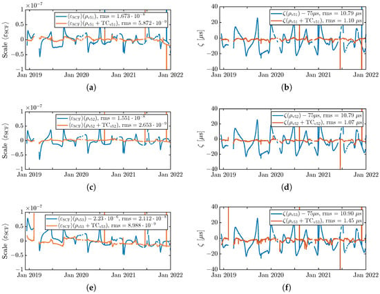
Figure 9. Comparison of scale and timeshift for LRI1B-v51, v52 and v53. Each subplot shows the results from the raw data product (blue) and including the Thermal Coupling (TC) in red. Left column: Scale factor $⟨{\epsilon }_{\mathrm{SCF}}⟩$ for different frequency models v51, v52, v53. Right column: corresponding timeshift $\zeta$. From top to bottom: v51, v52, v53. Outliers removed for computing the rms values. (a) Scale factor $⟨{\epsilon }_{\mathrm{SCF}}⟩$ for v51. (b) Timeshift $\zeta$ for v51. Blue line shifted by 75 $\mathsf{\mu }$$\mathrm{s}$. (c) Scale factor $⟨{\epsilon }_{\mathrm{SCF}}⟩$ for v52. (d) Timeshift $\zeta$ for v52. Blue line shifted by 75 $\mathsf{\mu }$$\mathrm{s}$. (e) Scale factor $⟨{\epsilon }_{\mathrm{SCF}}⟩$ for v53. Blue line shifted by $-2.23\times {10}^{-6}$. (f) Timeshift $\zeta$ for v53. Blue line shifted by 75 $\mathsf{\mu }$$\mathrm{s}$.

Here, the scale factor shows some seasonal patterns with an approximately three-month period and with an amplitude of $\pm 0.05$ ppm in all products; in v51 and v52 around zero, and in v53 around a $2.2$ ppm offset. The blue trace in the lower left panel for v53 also includes the exponential decay shown in Figure 3. The timeshift in the right panels exhibits a 75 $\mathsf{\mu }$$\mathrm{s}$ offset and seasonal variations with $\pm 25$ $\mathsf{\mu }$$\mathrm{s}$ amplitude for all three products.

We note that the variations in the red traces of Figure 8 with approximately 6 $\mathsf{\mu }$$\mathrm{m}$ rms could be explained to a large extent with a daily varying scale and timeshift shown in Figure 9. However, if these peaks and dips forming the seasonal variations with $\pm 0.05$ ppm or equivalently $\pm 14$ $\mathrm{M}$Hz amplitude are physical variations in the laser and the cavity resonance frequency, we would expect to see such variations in the laser telemetry and thus the telemetry-based laser frequency ${\nu }^{\mathrm{TME}}\left(t\right)$. We also lack an explanation for variations in the timeshift between KBR and LRI. A static timeshift could be produced by delays and uncertainties in the timing chain, though the exact contributor is not yet found (see Appendix D for a brief discussion of the LRI time frame). Therefore, in the next section, we investigate if the postfit range error as defined by Equation (30) can be further reduced when temperature coupling coefficients are coestimated with the global scale and timeshift.

9. TC in KBR-LRI Residuals

Changes in the thermal environment at many spacecraft units predominantly appear at 1/rev and 2/rev frequencies and may alter the measured range. We identified two possible coupling mechanisms. First, the coupling could be in the laser frequency regime, like temperature changes of the cavity or USO acting as an additional scaling term. Secondly, errors could occur in the phase (pathlength) regime, e.g., due to temperature-dependent alignment of components or temperature-driven effects in the electronics. In this section, we estimate linear coupling factors for different temperature sensors, with units of $1/\mathrm{K}$ for the (fractional) frequency regime and $\mathrm{m}/\mathrm{K}$ for the phase regime, such that the residuals between LRI and KBR are further minimized. We call the sum of these two corrections the Thermal Coupling (TC). The TC coefficients and the global scale and time shift are estimated simultaneously so that the postfit residuals

$${\tilde{\rho }}_{\mathrm{err},\mathrm{v}5\mathrm{X}}^{\mathrm{post}-\mathrm{TC}}\left(t\right)=\left(1+⟨{\epsilon }_{\mathrm{SCF}}^{\mathrm{glo}}⟩\right)·{\tilde{\rho }}_{\mathrm{LRI},\mathrm{v}5\mathrm{X}}^{\mathrm{inst}}(t+{\zeta }^{\mathrm{glo}})-{\tilde{\rho }}_{\mathrm{KBR}}^{\mathrm{inst}}\left(t\right)-{\tilde{\rho }}_{\mathrm{KBR}}^{\mathrm{FV}}\left(t\right)-{\tilde{\rho }}_{\mathrm{TC}}\left(t\right)$$

(32)

are minimized. We define the TC as

$${\tilde{\rho }}_{\mathrm{TC}}\left(t\right)=\sum _i\delta {\tilde{\rho }}_{\mathrm{KBR}-\mathrm{LRI},i}^{\mathrm{freq}}\left(t\right)+\sum _i\delta {\tilde{\rho }}_{\mathrm{KBR}-\mathrm{LRI},i}^{\mathrm{phase}}\left(t\right),$$

(33)

where we account for the two different error coupling mechanisms and i denotes contributions from different temperature sensors $T_i\left(t\right)$. In case of the frequency-domain coupling, we define

$$\delta {\tilde{\rho }}_{\mathrm{KBR}-\mathrm{LRI},i}^{\mathrm{freq}}\left(t\right)=\mathrm{HPF}\left(L\left(t\right)·\left(c_{1,i}·T_i\left(t\right)+c_{2,i}·{\dot{T}}_i\left(t\right)\right),0.08\mathrm{MHz}\right),$$

(34)

which is justified by Equation (13), which has shown that scale errors ($c_{1,i}·T_i\approx {\epsilon }_{\mathrm{SCF}}$) couple with the absolute distance $L\approx 220 \mathrm{k}\mathrm{m}$ into the measured range and where the high-pass filter is employed to remove long-term drifts in accordance and for the same reasoning as in Equation (29). The $\mathrm{c}\mathrm{m}$-precision of the GPS-based absolute range L obtained from GNI1B-v04 is sufficient here because the coupling coefficients are below 10⁻⁵, which yields a precision of 0.1 $\mathsf{\mu }$$\mathrm{m}$ or better. The coefficients $c_{1,i}$ and $c_{2,i}$ have units of $1/\mathrm{K}$ and $\mathrm{s}/\mathrm{K}$, respectively. They can be converted to approximate equivalent laser frequency couplings in units of $\mathrm{Hz}/\mathrm{K}$ by multiplying with ${\nu }_0\approx 281\mathrm{T}\mathrm{Hz}$. The second term $c_{2,i}·{\dot{T}}_i$ in Equation (34) is the first-order linearization of a potential timeshift due to propagation time from temperature changes to the measurement (cf. Equation (14)). This timeshift can be computed by ${\zeta }_{T_i}=c_{2,i}/c_{1,i}$. It should be noted that a positive sign of ${\zeta }_{T,i}$ is not violating causality because the timeshift can always be regarded as a modulus with regard to the orbital frequency.

The phase-domain TC contributors read

$$\delta {\tilde{\rho }}_{\mathrm{KBR}-\mathrm{LRI},i}^{\mathrm{phase}}\left(t\right)=\mathrm{HPF}\left(c_{1,i}·T_i\left(t\right)+c_{2,i}·{\dot{T}}_i\left(t\right),0.08\mathrm{MHz}\right),$$

(35)

where the coefficients $c_1$ and $c_2$ have the units $\mathrm{m}/\mathrm{K}$ and $\mathrm{s}·\mathrm{m}/\mathrm{K}$, respectively. Again, a potential time shift is linearized and the same high-pass filter used for the error range (cf. Equation (29)) removes frequencies below 1 CPR, i.e., long-term drifts, but maintains 1 CPR, which has high relevance for the scale factor.

We decompose the temperature $T_i$ into $T_i=T_{\mathrm{AC},i}+T_{\mathrm{DC},i}$ by high- and low-pass filtering, again using the same cutoff frequency of $0.08$ $\mathrm{M}$Hz. There are 161 thermistors $T_i$ per spacecraft (SC), and the data is retrieved from so-called OFFRED data and downsampled to $3.3\mathrm{MHz}$ as well. We expect that the DC parts are more likely to cause variations in the frequency regime, whereas the AC parts cause $\mathrm{m}/\mathrm{K}$-couplings. This is because the DC part contains a large static offset with only slight variations, which would imply a constant and hence irrelevant offset in ${\tilde{\rho }}_{\mathrm{err}}$, if the phase-domain coupling would apply, but prominent 1/rev tones in case of the frequency coupling due to the multiplication with L in Equation (34).

An optimization algorithm iteratively picks a single temperature sensor that minimizes the postfit range error ${\tilde{\rho }}_{\mathrm{err},\mathrm{v}5\mathrm{X}}^{\mathrm{post}-\mathrm{TC}}$ the most. To do so, the parameters $c_{1,i}$ and $c_{2,i}$ from Equations (34) and (35) are determined for both components $T_{\mathrm{AC},i}$ and $T_{\mathrm{DC},i}$ of each temperature sensor $T_i$ in every iteration and the minimization gain, i.e., the residual rms of KBR-LRI with this particular correction term divided by the residual rms without, is computed. For every iteration, the parameters of all the previously added sensors as well as $⟨{\epsilon }_{\mathrm{SCF}}^{\mathrm{glo}}⟩$ and ${\zeta }^{\mathrm{glo}}$ are always coestimated alongside the newly added sensor. Hence, we extend the design matrix for the least squares minimization by two columns per iteration.

The algorithm stops after adding five sensors, giving 12 coefficients in total: two global scale $⟨{\epsilon }_{\mathrm{SCF}}^{\mathrm{glo}}⟩$ and timeshift ${\zeta }^{\mathrm{glo}}$ biases for the whole period and two coefficients for each selected temperature sensor according to Equations (33)–(35). The estimated constants for scale and timeshift are shown in the last two columns of Table 3. The corresponding thermistor coefficients are shown in Table 4a–c for the ranging products v51, v52, and v53, respectively. The resulting residuals ${\tilde{\rho }}_{\mathrm{err},\mathrm{v}5\mathrm{X}}^{\mathrm{post}-\mathrm{TC}}$ are also shown in Figure 8 (yellow). The subtraction of the full TC model reduces the KBR-LRI rms residuals to a level of $1.6$ $\mathsf{\mu }$$\mathrm{m}$ (v51), $1.0$ $\mathsf{\mu }$$\mathrm{m}$ (v52) and $2.3$ $\mathsf{\mu }$$\mathrm{m}$ (v53). Especially in the case of v52, this is close to the expected KBR noise limit of $0.4$ $\mathsf{\mu }$$\mathrm{m}$ rms (cf. Equation (31)).

Table 4. Thermal Coupling parameters. The index i denotes the order of importance, i.e., the gain in reducing the rms residuals. The $\delta \tilde{\rho }$ type denotes the coupling in phase or frequency regime. Thus, the unit of $c_1$ is $\mathrm{m}/\mathrm{K}$, if the AC-component was used and $1/\mathrm{K}$, if the DC-component was used. The coefficient $c_2$ has units $\mathrm{s} \mathrm{m}/\mathrm{K}$ (AC) or $\mathrm{s}/\mathrm{K}$ (DC). The last column ${\zeta }_T=c_2/c_1$ describes the timeshift of the temperature data in seconds.

(a) v51: Telemetry-Based Laser Frequency Model ${\mathit{\nu }}_{1/2}^{\mathbf{TM}}$
$\mathit{i}$	SC	Sensor ID	Ascii Name	${\mathit{T}}_{\mathrm{AC}}/{\mathit{T}}_{\mathrm{DC}}$	$\mathbf{\delta }\tilde{\mathbf{\rho }}$type	${\mathit{c}}_{\mathbf{1}}$	${\mathit{c}}_{\mathbf{2}}$	${\mathit{\zeta }}_{\mathit{T}}$[$\mathrm{s}$]
1	GF-1	THT10013	SaMzPx	AC	phase	$-1.127\times {10}^{-7}$	$-6.240\times {10}^{-6}$	55.4
2	GF-2	THT10133	BatTrp	AC	phase	$-1.173\times {10}^{-5}$	$-1.379\times {10}^{-3}$	117.6
3	GF-1	THT10144	Pr21	DC	freq	$-1.642\times {10}^{-9}$	$-1.501\times {10}^{-6}$	914.0
4	GF-1	THT10022	LriLpcMy	DC	freq	$2.640\times {10}^{-9}$	$1.182\times {10}^{-6}$	447.9
5	GF-1	THT10143	Oct11	AC	phase	$4.153\times {10}^{-6}$	$-9.814\times {10}^{-4}$	−236.3
(b) v52: Exponential Cavity Frequency Decay Model ${\mathit{\nu }}_{\mathrm{R}}^{\mathbf{Cav}}$
$\mathit{i}$	SC	Sensor ID	Ascii Name	${\mathit{T}}_{\mathrm{AC}}/{\mathit{T}}_{\mathrm{DC}}$	$\mathit{\delta }\tilde{\mathit{\rho }}$type	${\mathit{c}}_{\mathbf{1}}$	${\mathit{c}}_{\mathbf{2}}$	${\mathit{\zeta }}_{\mathit{T}}$[$\mathrm{s}$]
1	GF-1	THT10013	SaMzPx	AC	phase	$-1.302\times {10}^{-7}$	$6.194\times {10}^{-6}$	−47.6
2	GF-2	THT10138	MepFrontPy	AC	phase	$-2.238\times {10}^{-7}$	$5.403\times {10}^{-5}$	−241.4
3	GF-1	THT10007	GpsOccAnt	DC	freq	$1.513\times {10}^{-11}$	$-2.382\times {10}^{-8}$	−1573.9
4	GF-2	THT10089	LriOba	AC	phase	$-1.080\times {10}^{-5}$	$1.091\times {10}^{-3}$	−101.0
5	GF-2	THT10113	LriLas	DC	freq	$1.049\times {10}^{-10}$	$-1.121\times {10}^{-6}$	−10,689.7
(c) v53: Pre-Calibrated Fixed Frequency Value ${\mathit{\nu }}_{\mathbf{0}}$
$\mathit{i}$	SC	Sensor ID	Ascii Name	${\mathit{T}}_{\mathbf{AC}}/{\mathit{T}}_{\mathbf{DC}}$	$\mathit{\delta }\tilde{\mathit{\rho }}$type	${\mathit{c}}_{\mathbf{1}}$	${\mathit{c}}_{\mathbf{2}}$	${\mathit{\zeta }}_{\mathit{T}}$[$\mathrm{s}$]
1	GF-2	THT10032	SaMzMx	AC	phase	$-1.022\times {10}^{-7}$	$1.923\times {10}^{-5}$	−188.2
2	GF-2	THT10052	AccPanel	DC	freq	$-9.162\times {10}^{-9}$	$-4.827\times {10}^{-6}$	526.8
3	GF-2	THT10138	MepFrontPy	AC	phase	$-4.996\times {10}^{-6}$	$8.787\times {10}^{-4}$	−175.9
4	GF-2	THT10157	Oct22	DC	freq	$5.288\times {10}^{-10}$	$3.349\times {10}^{-7}$	633.4
5	GF-2	THT10052	AccPanel	AC	phase	$8.433\times {10}^{-5}$	$-3.014\times {10}^{-3}$	−35.7

We observe that in the first iteration, solar array minus z sensors (SaMz**) were chosen in all three cases, which are attached to the zenith-pointing solar panels. We expect that the underlying satellite interior’s thermal environment is highly correlated to these sensors because the solar arrays are directly heated by the sun and thus exhibit large temperature variations. Figure 10 shows the dominant 1/rev and 2/rev amplitudes of these particular sensors. A 1/rev amplitude of 80 $\mathrm{K}$ results in a tone error of roughly 8 $\mathsf{\mu }$$\mathrm{m}$ at 1/rev, as apparent from the $c_1\approx 0.1 \mathsf{\mu }\mathrm{m}/\mathrm{K}$ coupling factors in the first rows of Table 4a–c.

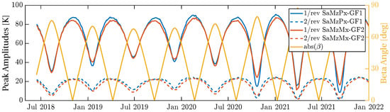
Figure 10. Peak amplitudes at 1/rev and 2/rev frequencies for SaMzPx of GF-1 (blue) and SaMzMx of GF-2 (orange), which are the most dominant TC contributors. The yellow curve shows the absolute value of the $\beta$-angle between the orbital plane and the sun. The sinusoidal 1/rev and 2/rev temperature amplitudes are much higher when the $\beta$-angle is close to zero, i.e., when the sun is in the orbital plane.

We highlight that most temperature sensors inside the spacecraft are highly correlated. Thus, there might be other sets of five sensors that could produce very similar results.

For verifying the TC, the daily scale and timeshift of KBR and LRI are computed again by using the LRI1B-v5X ranging products, but now we subtract the TC model ${\tilde{\rho }}_{\mathrm{TC}}\left(t\right)$ beforehand. The new scale and timeshift are shown in orange also in Figure 9. They clearly show fewer seasonal variations than the blue curves without TC. The best performance, by means of reducing the variations in the daily scale factor estimate $⟨{\epsilon }_{\mathrm{SCF}}⟩$ in the KBR-LRI differences, is achieved when using v52, which is based on the exponential cavity frequency model in combination with the TC. Here, the rms variations of the scale factor $⟨{\epsilon }_{\mathrm{SCF}}⟩\left({\rho }_{\mathrm{v}}52\right)$ are reduced from $1.551\times {10}^{-8}$ to $2.653\times {10}^{-9}$. Moreover, the corresponding timeshift $\zeta ({\rho }_{\mathrm{v}}52+{\mathrm{TC}}_{\mathrm{v}}52)$ exhibits low variations of about 1 $\mathsf{\mu }$$\mathrm{s}$ when including the TC correction ${\tilde{\rho }}_{\mathrm{TC}}$.

We emphasize that the TC parameters shown in Table 3 and Table 4c can also be used to correct the LRI1B-v04 dataset by SDS. However, one has to revert the effects of the daily $⟨{\epsilon }_{\mathrm{SCF}}^{\mathrm{SDS}}⟩$ and $\zeta$ beforehand, which are already applied in LRI1B-v04. The timeshift $\zeta$ can be extracted by forming the difference of the time offsets (eps_time) provided in CLK1B and LLK1B.

If we assume that ${\tilde{\rho }}_{\mathrm{TC}}$ is mainly caused by the KBR instrument, e.g., due to the stable cavity resonance frequency and thermally induced KBR antenna phase center variations, the most precise intersatellite ranging dataset is given by LRI1B-v52 with scale $⟨{\epsilon }_{\mathrm{SCF}}^{\mathrm{glo}}⟩=$−3.810 × 10⁻⁹ $\approx -1 \mathrm{MHz}$, timeshift ${\zeta }^{\mathrm{glo}}=67.95 \mathsf{\mu }\mathrm{s}$, and without subtracting ${\tilde{\rho }}_{\mathrm{TC}}$.

Since the OFFRED thermistor data is not publicly available, we provide the $0.5$ Hz ranging data product LRI1B-v52 and the corresponding TC ranging correction called RTC1B-v52 (Range Thermal Coupling) (see Data Availability Statement below).

10. Discussion of Results and Alternative Approaches for Future Missions

The frequency of the LRI laser is needed to convert phase to range. Any error or uncertainty can be considered a scale error in the range measurement. Currently, the LRI scale or absolute frequency is estimated daily by correlating KBR range with LRI range. One goal of the methods presented in this paper is to derive an independent and reliable model for the absolute laser frequency ${\nu }_{\mathrm{R}}$ of the LRI. Such models would be needed if KBR data is missing, e.g., if the second IPU on the GF-2 satellite would become unavailable. Moreover, because the LRI processing becomes less dependent on the KBR, measurement errors in the KBR would not affect the LRI data anymore. Furthermore, in a future mission, there will likely be only a single LRI-like ranging instrument which requires a new processing scheme. There are several options for determining the absolute laser frequency for these missions, which will be discussed briefly in the following and are summarized in Table 5.

Table 5. Comparison table of the methods to determine the absolute laser frequency ${\nu }_{\mathrm{R}}$ or scale factor ${\epsilon }_{\mathrm{SCF}}$ as presented in Section 10.

Method	Accuracy	Pros/Cons
Telemetry model	60 MHz (200 ppb)	+ No changes of flight hardware required − Thorough calibration of laser and cavity required − Low accuracy, may be a backup solution
Cross-Correlation to MWI		− Estimated frequency susceptible to ranging tone errors in MWI and LRI − Not feasible in future missions without MWI
Estimation during GFR		+ no hardware changes − laser frequency highly correlated to $C_{2,0}$ gravity coefficient − susceptible to instrument tone errors and to errors from GFR (e.g., temporal aliasing, gravity background model errors) − may have correlations to other empirical parameters (e.g., for accelerometer)
Iodine Cell	1 kHz ($3\times {10}^{-3}$ ppb)	+ Highest accuracy − High mass and (optical) power demands
FSR Readout	3 MHz (10 ppb)	+ Sufficient accuracy + Minor changes to existing optoelectronics, additional eletronics for readout of EOM driver required

The telemetry-based models ${\nu }_{1/2}^{\mathrm{TME}}$, which includes the empirical correction term ${\nu }_{1/2}^{\mathrm{emp}}$ from in-flight measurements, reached an accuracy of approximately $60\mathrm{MHz}\approx 200 ppb$ (see Figure 7). Because the laser is thermally coupled to the satellite platform, temperature variations of the surrounding units couple into the setpoint-based model but not into the true frequency determined by the cavity. We emphasize that the LRI is a technology demonstrator and the calibration of the laser frequency had only a moderate priority. However, the authors assume that such accuracy could also be achievable in a future mission from on-ground calibrations only if the laser is characterized more thoroughly, in particular, if the drift of 40 $\mathrm{M}$Hz/$\mathrm{yr}$ of the laser setpoint in ${\nu }_{1/2}^{\mathrm{emp}}$ is calibrated. Additionally, one might attempt to characterize the cavity frequency exponential decay on-ground and derive an estimate for the flight phase.

An alternative to determining the frequency from in-flight telemetry is to coestimate it during gravity field recovery (GFR), as it is usually done for the accelerometer scales and biases [24,25]. However, any LRI scale uncertainty mainly manifests at 1/rev and 2/rev frequencies, where the GFR processing strategies often introduce empirical parameters that partly absorb the scale factor [25]. Furthermore, the estimated scale is highly correlated with the $C_{2,0}$ spherical harmonics coefficient, which is mainly measurable at 1/rev and 2/rev frequencies and not estimated reliably in GFR [25]. We would expect that LRI errors from a scale factor uncertainty would be at the level of the postfit residuals of GFR, which are much higher than the LRI requirements of 10⁻⁷ or 10⁻⁸ (cf. Section 3).

A well-known and broadly used approach to obtain a well-defined absolute laser frequency relies on iodine spectroscopy, in which the hyperfine transition line of an iodine molecule is used as an absolute reference for a laser lock [26]. This technology has also been used for calibrating the LRI RLUs (cf. Appendices Appendix A and Appendix B), and there are activities ongoing to qualify such setups for the space environment, see e.g., [27]. However, saturated Doppler-free spectroscopy is likely incompatible with the available optical power from Tesat RLUs used in the LRI so far. Hence, one would need to add optical amplifiers, which significantly increase the complexity and electric power consumption. Laboratory experiments showed absolute frequency repeatability levels below $1 \mathrm{kHz}\approx$ 3 × 10⁻³ $\mathrm{ppb}$ [27]. Thus, this method is probably the most accurate mean to fix or determine the scale factor. Optionally, there is the possibility for a hybrid lock by using both a conventional PDH lock to an optical cavity and a spectroscopic locking to an iodine reference. This hybrid lock combines the stability of the cavity at high Fourier frequencies, and the absolute laser frequency knowledge through the molecular reference [28].

Another approach for measuring the cavity resonance frequency is based on an extension of the PDH lock [29]. Adding an additional tone (scale factor tone) at a few $\mathrm{M}\mathrm{Hz}$ frequency together with upper and lower sidebands with the approximate free spectral range (FSR) separation enables the readout of the actual cavity FSR with regard to the applied sidebands. The frequency of these sidebands is derived coherently from the USO as the two tones and LRP time. After determination of the USO frequency during precise orbit determination, this technique can provide an estimate for the FSR frequency of the cavity. The cavity resonance frequency and FSR are linearly related to each other through $\nu =n_{\mathrm{mode}}·\mathrm{FSR}+\mathrm{offset}$, where the mode number $n_{\mathrm{mode}}$ is an integer mode number. The offset must be calibrated on-ground [30]. The principle has been demonstrated in laboratory experiments with an accuracy of roughly $3\mathrm{MHz}\approx 10 \mathrm{ppb}$. It is noteworthy that the scale factor tone and its sidebands have little influence on the conventional PDH readout [30,31]. The advantage of this technique is that only minor changes to existing flight hardware are needed, e.g., the use of $\mathrm{GHz}$ electro-optical modulators (EOMs) instead of $\mathrm{MHz}$. However, additional RF electronics and an additional processing unit for the readout are required. The FSR-readout is currently the most probable solution for upcoming gravity missions.

11. Conclusions

In this paper, the methodology as presented by [14] to derive a precise range from raw interferometric phase measurements was applied to in-flight data of the GRACE-FO LRI instrument. Based on that work, we derived the two dominant error terms, namely a time-variable scaling of the laser frequency, expressed through a scale factor ${\epsilon }_{\mathrm{SCF}}$, and a timeshift $\zeta$ of the LRI measurement with regard to the reference measurement is given by the KBR. Importantly, variations in ${\epsilon }_{\mathrm{SCF}}$ couple into the range proportionally to the absolute distance L between the two satellites. The scale ${\epsilon }_{\mathrm{SCF}}$ and timeshift $\zeta$ parameters can easily be compromised if errors in the range measurement at 1/rev and 2/rev frequencies are present.

In the second part, three different models by which to calculate the in-flight laser frequency were shown, which are largely independent of KBR measurements, once the model parameters are determined. Based on these models, we derive three versions of an LRI1B-equivalent data product, namely v51, v52, and v53. The first method (v53) uses a constant, nominal laser frequency ${\nu }_0$, which was chosen early before launch, and without sophisticated analysis because it was clear that the numerical values serve as a start value for the subsequent and accurate refinement utilizing cross-calibration. Thus, v53 is, in principle, a prerelease for the official LRI1B-v04 dataset. The latter is further refined by daily cross-calibrating LRI and KBR ranging data, i.e., estimating scale $⟨{\epsilon }_{\mathrm{SCF}}⟩$ and time-shift $\zeta$ on a daily basis. The daily scale factor or frequency ${\nu }^{\mathrm{SDS}}$ determined from the cross-calibration revealed seasonal variations and a settling effect, which we attribute to the optical reference cavity and which might be related to aging of the ULE cavity spacer material as reported in [19]. We use an exponential decay function (cf. Equation (22)) to describe this settling effect and to form v52. The v51 dataset uses a laser frequency model derived from LRI laser and temperature telemetry. One can relate the lasers’ control loop setpoints and temperatures to the output frequency by using linear coupling factors, which were calibrated on ground before launch. The setup of the preflight calibration measurements was explained, and the calibration factors were provided. The initial ${\nu }^{\mathrm{TM}}$-model from on-ground calibrations was then compared to four years of in-flight data of the GRACE-FO mission. It was found that the ${\nu }^{\mathrm{TM}}$ model frequency or, more precisely, the setpoints of the laser control loops drift over time by roughly 40 $\mathrm{M}$Hz/yr. Furthermore, two steps were observed when the lasers were operated in nonnominal conditions. The physical reason for the drift could be a consequence of aging effects of the NPRO crystal or electronics. However, although the exact reason remains unknown, we compensate for the drift and steps with an empirical model here. We observed that this telemetry-based model ${\nu }_{1/2}^{\mathrm{TME}}={\nu }_{1/2}^{\mathrm{TM}}-{\nu }_{1/2}^{\mathrm{emp}}$ of the laser frequency does not show seasonal variations, indicating that the seasonal variations of the frequency ${\nu }^{\mathrm{SDS}}$ are not actual changes in the laser frequency. The v51 dataset uses this empirically corrected model ${\nu }_{1/2}^{\mathrm{TME}}$.

Afterward, we focused on analyzing residuals of the difference of KBR-LRI, which we call the range error. At first, the direct difference yields large prefit range errors ${\tilde{\rho }}_{\mathrm{err},\mathrm{v}5\mathrm{X}}^{\mathrm{pre}}$ of more than 25 $\mathsf{\mu }$$\mathrm{m}$ rms for all three v5X data sets. In the second step, the effect of a global scale factor $⟨{\epsilon }_{\mathrm{SCF}}^{\mathrm{glo}}⟩$ and a global timeshift ${\zeta }^{\mathrm{glo}}$ are subtracted, reducing the postfit residuals ${\tilde{\rho }}_{\mathrm{err},\mathrm{v}5\mathrm{X}}^{\mathrm{post}}$ to approximately $6 \mathsf{\mu }\mathrm{m}\mathrm{rms}$ in all three cases.

These postfit residuals could be explained by seasonal variations in the scale and timeshift as determined from daily cross-calibration of LRI with regard to KBR. However, because the telemetry-based frequency model ${\nu }^{\mathrm{TME}}$ does not show these seasonal variations, we described them with a Thermal Coupling (TC). We accounted for two TC mechanisms, one in the phase domain and one in the frequency domain. An algorithm to determine coupling coefficients for all temperature sensors on both spacecraft was explained, and equations to compute the TC were given. For each of the three datasets, a TC composed of 12 coefficients, which includes five temperature sensors, was derived. For each temperature sensor, we derived a linear coupling $c_1$ with units of $\mathrm{m}/\mathrm{K}$ (phase domain) or $1/\mathrm{K}$ (frequency domain) and a possible time delay ${\zeta }_T$. Furthermore, the two global parameters for the scale $⟨{\epsilon }_{\mathrm{SCF}}^{\mathrm{glo}}⟩$ and timeshift ${\zeta }^{\mathrm{glo}}$, which are constant over the whole mission span, were refined. We showed that the differences between LRI and KBR can be reduced from approximately 25 $\mathsf{\mu }$$\mathrm{m}$ rms to 1 $\mathsf{\mu }$$\mathrm{m}$ rms when using LRI1B-v52 including the TC. In all three cases, the dominant thermal coupling originates from thermistors attached to the zenith-facing solar array. An analysis of these thermistor timeseries’ revealed that their 1/rev and 2/rev amplitudes are highest when the angle $\beta$ between the orbital plane and the sun is close to zero, which occurs roughly every six months. The tone error magnitude of these sensors in the TC is on the order of $\pm 8$ $\mathsf{\mu }$$\mathrm{m}$.

We analyzed only the thermal effects that are not common in LRI and KBR, i.e., which appear in the KBR-LRI difference. Thus, the TC does not address potential common effects.

This paper introduced a new laser frequency model for the LRI, representing the current best knowledge of the cavity resonance frequency on GF-1. We showed that this resonance frequency is relatively stable after an initial exponential convergence. As apparent from daily KBR-LRI cross-calibration, seasonal variations can be explained with tone errors from a Thermal Coupling.

References

- Abich, K.; Abramovici, A.; Amparan, B.; Baatzsch, A.; Okihiro, B.B.; Barr, D.C.; Bize, M.P.; Bogan, C.; Braxmaier, C.; Burke, M.J.; et al. In-Orbit Performance of the GRACE Follow-on Laser Ranging Interferometer. Phys. Rev. Lett. 2019, 123, 031101. [Google Scholar] [CrossRef] [PubMed]
- Landerer, F.W.; Flechtner, F.M.; Save, H.; Webb, F.H.; Bandikova, T.; Bertiger, W.I.; Bettadpur, S.V.; Byun, S.H.; Dahle, C.; Dobslaw, H.; et al. Extending the Global Mass Change Data Record: GRACE Follow-On Instrument and Science Data Performance. Geophys. Res. Lett. 2020, 47, e2020GL088306. [Google Scholar] [CrossRef]
- Ghobadi-Far, K.; Han, S.C.; McCullough, C.M.; Wiese, D.N.; Yuan, D.N.; Landerer, F.W.; Sauber, J.; Watkins, M.M. GRACE Follow-On Laser Ranging Interferometer Measurements Uniquely Distinguish Short-Wavelength Gravitational Perturbations. Geophys. Res. Lett. 2020, 47, e2020GL089445. [Google Scholar] [CrossRef]
- Conklin, J.; Yu, T.; Guzman, F.; Klipstein, B.; Lee, J.; Leitch, J.; Numata, K.; Petroy, S.; Spero, R.; Ware, B. LRI TechnologySummary and Roadmap for Mass Change Mission; Technical Report; NASA Jet Propulsion Laboratory: Pasadena, CA, USA, 2020. Available online: https://science.nasa.gov/science-red/s3fs-public/atoms/files/LRI-Technology-Summary-and-Roadmap.pdf (accessed on 12 January 2023).
- Massotti, L.; Siemes, C.; March, G.; Haagmans, R.; Silvestrin, P. Next Generation Gravity Mission Elements of the Mass Change and Geoscience International Constellation: From Orbit Selection to Instrument and Mission Design. Remote Sens. 2021, 13, 3935. [Google Scholar] [CrossRef]
- Nicklaus, K.; Cesare, S.; Massotti, L.; Bonino, L.; Mottini, S.; Pisani, M.; Silvestrin, P. Laser metrology concept consolidation for NGGM. In Proceedings of the International Conference on Space Optics—ICSO 2018; Karafolas, N., Sodnik, Z., Cugny, B., Eds.; SPIE: Bellingham, WA, USA, 2019. [Google Scholar] [CrossRef]
- Nicklaus, K.; Voss, K.; Feiri, A.; Kaufer, M.; Dahl, C.; Herding, M.; Curzadd, B.A.; Baatzsch, A.; Flock, J.; Weller, M.; et al. Towards NGGM: Laser Tracking Instrument for the Next Generation of Gravity Missions. Remote Sens. 2022, 14, 4089. [Google Scholar] [CrossRef]
- Amaro-Seoane, P.; Audley, H.; Babak, S.; Baker, J.; Barausse, E.; Bender, P.; Berti, E.; Binetruy, P.; Born, M.; Bortoluzzi, D.; et al. Laser Interferometer Space Antenna. arXiv 2017, arXiv:1702.00786. [Google Scholar] [CrossRef]
- Kornfeld, R.P.; Arnold, B.W.; Gross, M.A.; Dahya, N.T.; Klipstein, W.M.; Gath, P.F.; Bettadpur, S. GRACE-FO: The Gravity Recovery and Climate Experiment Follow-On Mission. J. Spacecr. Rocket. 2019, 56, 931–951. [Google Scholar] [CrossRef]
- Sheard, B.S.; Heinzel, G.; Danzmann, K.; Shaddock, D.A.; Klipstein, W.M.; Folkner, W.M. Intersatellite laser ranging instrument for the GRACE follow-on mission. J. Geod. 2012, 86, 1083–1095. [Google Scholar] [CrossRef]
- Drever, R.W.P.; Hall, J.L.; Kowalski, F.V.; Hough, J.; Ford, G.M.; Munley, A.J.; Ward, H. Laser phase and frequency stabilization using an optical resonator. Appl. Phys. B 1983, 31, 97–105. [Google Scholar] [CrossRef]
- Thompson, R.; Folkner, W.M.; de Vine, G.; Klipstein, W.M.; McKenzie, K.; Spero, R.; Yu, N.; Stephens, M.; Leitch, J.; Pierce, R.; et al. A flight-like optical reference cavity for GRACE follow-on laser frequency stabilization. In Proceedings of the Joint Conference of the IEEE International Frequency Control and the European Frequency and Time Forum (FCS) Proceedings, San Francisco, CA, USA, 1–5 May 2011. [Google Scholar] [CrossRef]
- Yan, Y.; Müller, V.; Heinzel, G.; Zhong, M. Revisiting the light time correction in gravimetric missions like GRACE and GRACE follow-on. J. Geod. 2021, 95, 1–9. [Google Scholar] [CrossRef]
- Müller, V.; Hauk, M.; Misfeldt, M.; Müller, L.; Wegener, H.; Yan, Y.; Heinzel, G. Comparing GRACE-FO KBR and LRI Ranging Data with Focus on Carrier Frequency Variations. Remote Sens. 2022, 14, 4335. [Google Scholar] [CrossRef]
- Wegener, H.; Müller, V.; Heinzel, G.; Misfeldt, M. Tilt-to-Length Coupling in the GRACE Follow-On Laser Ranging Interferometer. J. Spacecr. Rocket. 2020, 57, 1362–1372. [Google Scholar] [CrossRef]
- Wen, H.Y.; Kruizinga, G.; Paik, M.; Landerer, F.; Bertiger, W.; Sakumura, C.; Bandikova, T.; Mccullough, C. GRACE-FO Level-1 Data Product User Handbook; JPL D-56935, Version of 11 September 2019; Jet Propulsion Laboratory: Pasadena, CA, USA, 2019. Available online: https://podaac-tools.jpl.nasa.gov/drive/files/allData/gracefo/docs/GRACE-FO_L1_Handbook.pdf (accessed on 12 January 2023).
- Heinzel, G.; Rudiger, A.; Schilling, R. Spectrum and Spectral Density Estimation by the Discrete Fourier Transform (DFT), Including a Comprehensive List of Window Functions and Some New Flat-Top Windows. Available online: https://pure.mpg.de/pubman/faces/ViewItemOverviewPage.jsp?itemId=item_152164 (accessed on 12 January 2023).
- Wen, H.Y. GRACE-FO Level-1 Release Notes, Revision of 22 May 2022. Available online: https://podaac-tools.jpl.nasa.gov/drive/files/allData/gracefo/docs/GRACE-FO_L1_ReleaseNotes.txt (accessed on 12 January 2023).
- Alnis, J.; Matveev, A.; Kolachevsky, N.; Udem, T.; Hänsch, T.W. Subhertz linewidth diode lasers by stabilization to vibrationally and thermally compensated ultralow-expansion glass Fabry-Pérot cavities. Phys. Rev. A 2008, 77, 053809. [Google Scholar] [CrossRef]
- Armano, M.; Audley, H.; Auger, G.; Baird, J.; Bassan, M.; Binetruy, P.; Born, M.; Bortoluzzi, D.; Brandt, N.; Caleno, M.; et al. LISA Pathfinder: First steps to observing gravitational waves from space. J. Phys. Conf. Ser. 2017, 840, 012001. [Google Scholar] [CrossRef]
- Pierce, R.; Stephens, M.; Kaptchen, P.; Leitch, J.; Bender, D.; Folkner, W.M.; Klipstein, W.M.; Shaddock, D.; Spero, R.; Thompson, R.; et al. Stabilized Lasers for Space Applications: A High TRL Optical Cavity Reference System. In Proceedings of the Conference on Lasers and Electro-Optics 2012, San Jose, CA, USA, 6–11 May 2012. [Google Scholar] [CrossRef]
- Nicklaus, K.; Herding, M.; Baatzsch, A.; Dehne, M.; Diekmann, C.; Voss, K.; Gilles, F.; Guenther, B.; Zender, B.; Böhme, S.; et al. Optical bench of the laser ranging interferometer on grace follow-on. In Proceedings of the International Conference on Space Optics—ICSO 2014; Sodnik, Z., Cugny, B., Karafolas, N., Eds.; International Society for Optics and Photonics, SPIE: Bellingham, WA, USA, 2017; Volume 10563, pp. 738–746. [Google Scholar] [CrossRef]
- Müller, L. Generation of Level 1 Data Products and Validating the Correctness of Currently Available Release 04 Data for the GRACE Follow-On Laser Ranging Interferometer. Master’s Thesis, Leibniz Universität Hannover, Hanover, Germany, 2021. [Google Scholar] [CrossRef]
- Helleputte, T.V.; Doornbos, E.; Visser, P. CHAMP and GRACE accelerometer calibration by GPS-based orbit determination. Adv. Space Res. 2009, 43, 1890–1896. [Google Scholar] [CrossRef]
- Klinger, B.; Mayer-Gürr, T. The role of accelerometer data calibration within GRACE gravity field recovery: Results from ITSG-Grace2016. Adv. Space Res. 2016, 58, 1597–1609. [Google Scholar] [CrossRef]
- Arie, A.; Schiller, S.; Gustafson, E.K.; Byer, R.L. Absolute frequency stabilization of diode-laser-pumped Nd:YAG lasers to hyperfine transitions in molecular iodine. Opt. Lett. 1992, 17, 1204–1206. [Google Scholar] [CrossRef]
- Döringshoff, K.; Schuldt, T.; Kovalchuk, E.V.; Stühler, J.; Braxmaier, C.; Peters, A. A flight-like absolute optical frequency reference based on iodine for laser systems at 1064 nm. Appl. Phys. B 2017, 123, 1–8. [Google Scholar] [CrossRef]
- Sanjuan, J.; Abich, K.; Blümel, L.; Gohlke, M.; Gualani, V.; Oswald, M.; Wegehaupt, T.; Schuldt, T.; Braxmaier, C. Simultaneous laser frequency stabilization to an optical cavity and an iodine frequency reference. Opt. Lett. 2021, 46, 360. [Google Scholar] [CrossRef]
- DeVoe, R.G.; Brewer, R.G. Laser-frequency division and stabilization. Phys. Rev. A 1984, 30, 2827–2829. [Google Scholar] [CrossRef]
- Rees, E.R.; Wade, A.R.; Sutton, A.J.; McKenzie, K. Absolute Frequency Readout of Cavity against Atomic Reference. Remote Sens. 2022, 14, 2689. [Google Scholar] [CrossRef]
- Rees, E.R.; Wade, A.R.; Sutton, A.J.; Spero, R.E.; Shaddock, D.A.; Mckenzie, K. Absolute frequency readout derived from ULE cavity for next generation geodesy missions. Opt. Express 2021, 29, 26014. [Google Scholar] [CrossRef] [PubMed]
- Misfeldt, M.; Müller, L.; Müller, V. Alternative GRACE-FO LRI Ranging Datasets: AEI-LRI1B-v52; Leibniz Universität Hannover: Hannover, Germany, 2022. [Google Scholar] [CrossRef]
- Schuldt, T.; Braxmaier, C.; Müller, H.; Huber, G.; Peters, A.; Johann, U. Frequency stabilized ND:YAG laser for space applications. In Proceedings of the International Conference on Space Optics—ICSO 2004; Costeraste, J., Armandillo, E., Eds.; SPIE: Bellingham, WA, USA, 2004. [Google Scholar] [CrossRef]
- Coherent, Inc. Prometheus—Ultra-Narrow Linewidth CW DPSS Green Laser; Coherent, Inc.: Santa Clara, CA, USA, 2022; Available online: https://www.coherent.com/content/dam/coherent/site/en/resources/datasheet/lasers/prometheus-ds.pdf (accessed on 12 January 2023).
- Riehle, F.; Gill, P.; Arias, F.; Robertsson, L. The CIPM list of recommended frequency standard values: Guidelines and procedures. Metrologia 2018, 55, 188–200. [Google Scholar] [CrossRef]
- Ware, B. LRI FM1 Datation Test Report; Project Internal Document; Jet Propulsion Laboratory, California Institute of Technology: Pasadena, CA, USA, 2018.
Disclaimer/Publisher’s Note: The statements, opinions and data contained in all publications are solely those of the individual author(s) and contributor(s) and not of MDPI and/or the editor(s). MDPI and/or the editor(s) disclaim responsibility for any injury to people or property resulting from any ideas, methods, instructions or products referred to in the content. |
© 2023 by the authors. Licensee MDPI, Basel, Switzerland. This article is an open access article distributed under the terms and conditions of the Creative Commons Attribution (CC BY) license (https://creativecommons.org/licenses/by/4.0/).