A Comparative Study of Different CNN Models and Transfer Learning Effect for Underwater Object Classification in Side-Scan Sonar Images

Abstract

With the development of deep learning techniques, convolutional neural networks (CNN) are increasingly being used in image recognition for marine surveys and underwater object classification. Automatic recognition of targets on side-scan sonar (SSS) images using CNN can improve recognition accuracy and efficiency. However, the vast selection of CNN models makes it challenging to select models for target recognition in SSS images. Therefore, this paper aims to compare different CNN models’ prediction accuracy and computational performance comprehensively. First, four traditional CNN models were applied to train and predict the same submarine SSS dataset using both the original model and models with transfer learning methods. Then, we examined and studied the prediction accuracy and computation performance of four CNN models. Results showed that transfer learning enhances the accuracy of all CNN models, with lesser improvements for AlexNet and VGG-16 and greater improvements for GoogleNet and ResNet101. GoogleNet has the highest prediction of accuracy (100% in the train dataset and 94.27% in the test dataset) and good computational difficulty. The findings of this work are useful for future model selection in target recognition in SSS images.

1. Introduction

Side-scan sonar (SSS) can detect seafloor geomorphology, seabed engineering structures, underwater objects, and seafloor geological phenomena by providing highly accurate underwater mosaics. It has significant application value in the field of marine geology. However, there is a high demand for researchers’ experience in identifying targets in SSS images. Due to the speckle noise and intensity inhomogeneity of SSS images, there are differences in the images interpreted by different experienced personnel. In addition, the large amount of image processing work could be more conducive to efficiency and accuracy. Therefore, there is an urgent need for methods to improve accuracy and efficiency for automatic interpretation and recognition in SSS images.

In recent years, various artificial intelligence (AI) algorithms have been used in many applications in the field of geology, such as seafloor sediment accumulation prediction [1], oil and gas reserves forecast [2], seafloor substrate classification [3], geological drilling [4,5,6,7,8], geological hazards prediction [9,10,11], etc. Among these applications, convolutional neural network (CNN) was also widely used for target recognition in SSS images. Automatic recognition and prediction of SSS images using CNN can significantly increase efficiency and accuracy.

To study the applicability of different CNN models in target recognition in SSS images, the CNN-based networks DCNN [12], ECNet [13], YOLOv3 [14], VGG-19, and ResNet50 [15] were all used for recognition and obtained good prediction accuracies. To reduce the impact of a small amount of data on prediction accuracy, Sung et al. [16] proposed a GAN-based method for generating realistic SSS images to address the problem of the insufficient data volume of SSS images of the seafloor, which can generate images of SSS image types to help train the model. Few-shot learning [17] was also used for modeling to reduce the effect of small training samples of SSS images. As for the SSS datasets, Huo et al. [18] proposed a dataset named SeabedObjects-KLSG to enrich the SSS image data resource. The composition of CNN model structures can take many forms, and there are no less than 10 well-established models that are widely used in a variety of fields. Although numerous CNN models have been applied to SSS image target recognition and claimed to have good accuracies, the prediction accuracy between the models has not been significantly compared and analyzed. Therefore, choosing the appropriate model among the many CNN models for target recognition in SSS images is very important.

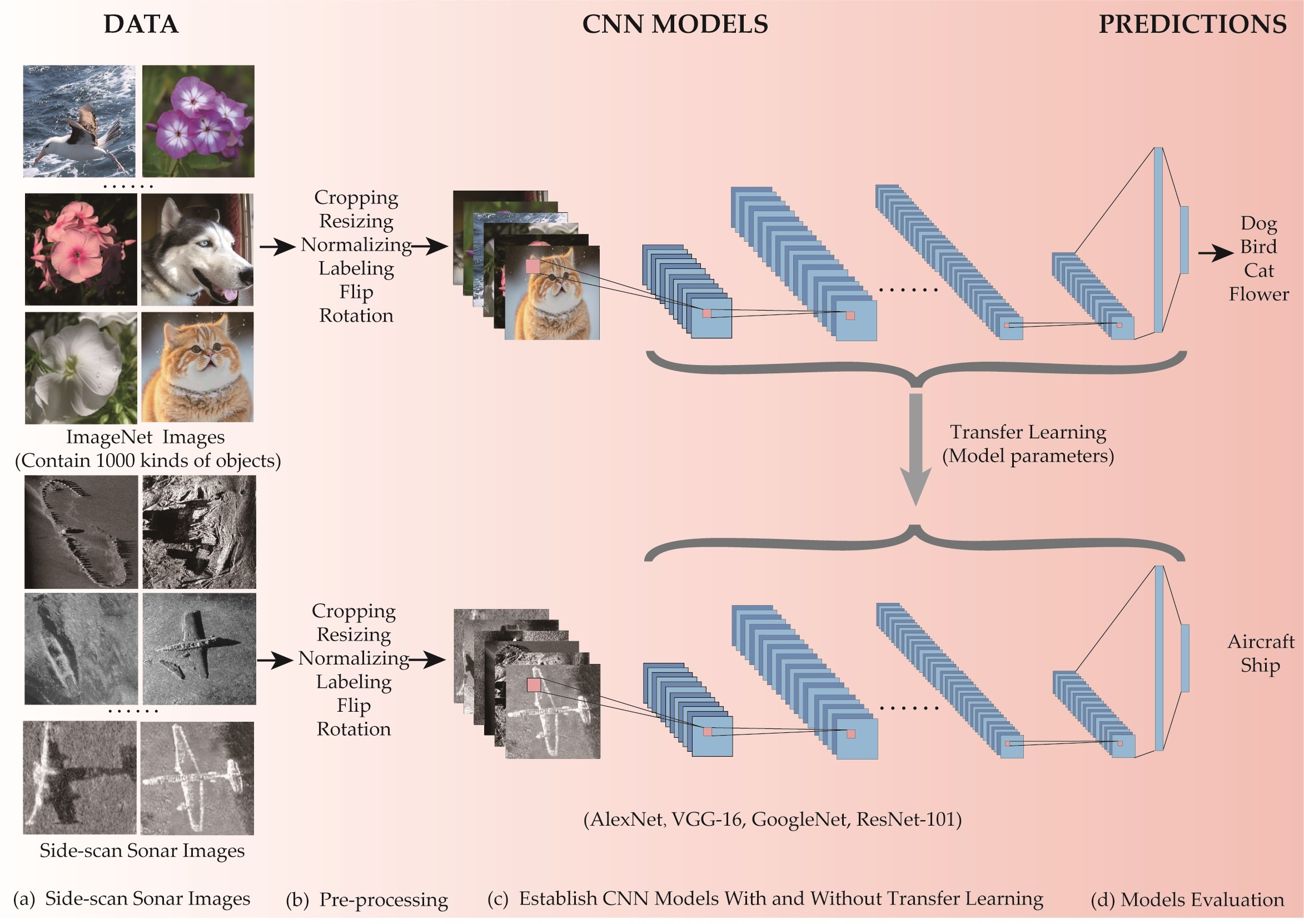
In this paper, we evaluated eight CNN models (AlexNet, VGG-16, GoogleNet, and ResNet101, with and without transfer learning) to predict the SeabedObjects-KLSG dataset, and we compared and analyzed the differences in the prediction accuracy of different models for SSS images. A comprehensive analysis of each model’s computational efficiency and difficulty was also presented. The main improvements are as follows: (1) We investigated the degree of influence of transfer learning on CNNs with different structures and the reasons for it. (2) We compared the prediction accuracy of different CNN models on the SSS dataset and analyzed the reasons for the different degrees of influence. (3) We proposed CNN model recommendations for different computational cases.

2. Applied CNN Models

Convolutional neural network (CNN) is a fundamental component of deep learning, primarily through the convolution and pooling of multidimensional matrices to reduce the number of operations, improve computational performance, and choose relevant input data. Due to its remarkable capacity to manage multidimensional data, CNN is typically utilized for detecting and analyzing image data.

Take a single-channel grayscale image as an example (Figure 1). When the image is input, it can be regarded as a three-dimensional matrix for processing. When the input image is convolved, a matrix of a specific size (usually 3 × 3 or 5 × 5) is used as a filter. A new matrix is obtained by matrix multiplication with the input image matrix. The filter can have multiple groups and the new matrix will have many groups. This operation is called convolution, and the new matrixes are obtained as convolution layers. The pooling procedure is equivalent to employing a tiny filter, in which the input layer is divided into several areas based on the size of the filter. Typically, there are two approaches for maintaining valid information in a region: the maximum value or the average value. The related methods are known as maximum pooling and average pooling, respectively. The pooling layers are acquired thereafter. The combination of convolution and pooling layers may be reused, and different convolution settings can be specified depending on the quantity of data and image attributes. Convolution and pooling are comparable to extracting valid information from input photos and reducing background noise. Then, all legitimate data must be included prior to the final output result. First, the convolutional layer needs to be downscaled to a two-dimensional matrix. Then, one or more layers of full concatenation are performed to output the desired data type.

Since LeCun [20] developed LeNet in 1998, CNN models were gradually applied to various scenarios, such as image processing and image segmentation. Among these CNN models, some networks are very classic due to their excellent generality and accuracy, such as AlexNet [21], VGGNet [22], ResNet [23], and GoogleNet [24]. Each CNN network used in this paper will be described in detail in the following sections.

2.1. AlexNet

Alex [21] proposed AlexNet in 2012 and won first place in the 2012 ILSVRC competition. AlexNet has an eight-layer structure, with the first five layers convolutional and the last three fully connected layers. It requires an image with a resolution of 227 × 227 as input and the classification information embedded in the image as output to perform network training. The AlexNet contains 630 million links, 60 million parameters, and 650,000 neural units, which made it a very sophisticated deep learning network in 2012, able to handle high-resolution image problems. Compared with previous CNNs, AlexNet mainly uses ReLU as the activation function for the first time, uses the Dropout method to avoid overfitting, and CUDA for accelerated training. These practices have significantly improved its computational efficiency and accuracy and advanced the process of deep learning.

2.2. VGG

VGG is a CNN model proposed by the Visual Geometry Group at Oxford [22]. The network was a related work at ILSVRC 2014, and its main accomplishment was demonstrating that increasing the depth of the network can affect the final performance of the network to some extent. It has been widely used as a typical CNN structure since it was proposed. VGGNet uses all 3 × 3 convolutional kernels and 2 × 2 pooling kernels to improve the performance by deepening the network structure, and successfully constructs a 16–19-layer deep CNN. The most commonly used is the 16-layer network, that is, VGG-16. VGG-16 is formed with 13 convolutional layers and 3 fully connected layers and contains 138 million parameters, which makes it very difficult to train. Compared with AlexNet, VGG expands toward deeper convolutional network layers and achieves better computational results but also brings a much larger number of parameters and computational difficulty.

2.3. GoogleNet

Christian Szegedy [24] from Google designed GoogleNet, the first Inception architecture, by reducing the number of layers and the amount of computation in deep neural networks. Unlike the previous tandem CNN, GoogleNet changed the CNN to be internally connected in parallel by introducing the Inception structure. As shown in Figure 2, when the data is processed using inception, it must pass through four paths with different convolutional kernels simultaneously; finally, the data are aggregated together as a new network layer. The structure of inception is the most significant difference between GoogleNet and traditional CNN networks. There are two major advantages of using the inception structure: first, the simultaneous convolution at multiple scales can extract features at different scales, which also results in more accuracy in the final classification judgment; second, the use of 1 × 1 convolution for dimensionality reduction reduces the computational complexity, and the amount of computation is significantly reduced when the number of features is reduced; then, convolution is carried out. Due to the advantages of inception, although GoogleNet has 22 network layers, which is more profound than AlexNet’s 8 layers or VGGNet’s 19 layers, it can achieve far better accuracy than AlexNet with only 5 million parameters (1/12 th of AlexNet’s parameters and 1/25 th of VGG-16’s parameters).

2.4. ResNet

ResNet is a residual network proposed by He [23] in 2015. In general, the deeper the network, the greater the quantity of information that can be obtained and the more robust the characteristics. Experiments indicate, however, that as the network becomes deeper, the optimization impact deteriorates and the accuracy of test data and train data decline. This phenomenon is a result of the gradient expansion and gradient vanishing issues produced by network deepening. To solve the degeneration problem in deep networks, it is possible to artificially make specific layers of a neural network skip the connection of neurons in the next layer and connect them in alternate layers, weakening the strong relationship between each layer. Such neural networks are called residual networks (ResNet).

As illustrated in Figure 3, the input data x is added with the original data x, and the F(X) is obtained after convolutional layer processing, compared with the traditional CNN structure. Subsequently, the valid information of two layers can be retained simultaneously, and the information loss caused by too many layers is simultaneously reduced. The CNN model built using this residual network can possess up to 100 layers or more. The model selected for the calculations in this paper is the ResNet101 model, which has 101 layers and 44 million parameters.

2.5. Transfer Learning

Transfer learning is the ability of a system to recognize and apply knowledge and skills learned in previous domains/tasks to novel domains/tasks. It was first proposed by Google Inc. [25] at the 2016 NIPS conference. Transfer learning takes a trained model base and trains it again, more accurately than training it from scratch, when encountering another similar problem. It is similar to how a human learns a skill and becomes more proficient when learning another similar skill. Therefore, when we need to train a CNN network, using a classical model previously pre-trained as a base and fine-tuning its structure and data for training again may provide better results than training from scratch.

In this paper, we also fine-tuned the CNN models pre-trained on the ImageNet dataset, which will be used for transfer learning. We added a fully connected layer with two output units after the fully connected layer of the classical CNN models (AlexNet, VGG-16, GoogleNet, or ResNet101) used to represent the output as a ship or an airplane. Consequently, we can then train the model using the train dataset on the SeabedObjects-KLSG dataset to obtain a more accurate SSS target recognition model.

3. Materials and Methods

3.1. Dataset

The data used in the experiments were obtained from an open real object dataset of SSS images named SeabedObjects-KLSG [18]. This open dataset contains 385 ship images and 62 airplane images. The sonar images were obtained with several sonar equipment suppliers, including Lcocean, Hydro-tech Marine, Klein Marine, Tritech, and EdgeTech, and through a decade of accumulation.

Some sample images of the SeabedObjects-KLSG dataset can be seen in Figure 4. It is clear that each SSS image is distinct, as are the images of the same airplanes or ship. The degree of brightness, size, sharpness, form, and damage to the ship and aircraft varies from image to image. We will utilize CNN to detect the information inherent inside photos through modeling.

3.2. Experimental Steps

As illustrated in Figure 5, the experimental steps mainly include data pre-processing, data augmentation, dataset partitioning, CNN model establishing, and accuracy comparison. Specific descriptions of steps are described in the following section.

3.2.1. Data Pre-Processing

The SSS images need to be pre-processed to meet the input requirements of the CNN training data before the modeling computation. The primary operations performed on the images consist of center cropping, resizing, normalizing, and labeling.

It is recommended to center crop the image using the center of the image as the base in order to better emphasize the subject of the underwater object and decrease the effect of the seabed. After cropping, the sonar images were uniformly resized to 227 × 227 pixels for AlexNet and 224 × 224 pixels for other CNN models to meet the input size requirements of the classical CNN networks used in the paper. Normalization can organize the data in the three channels of the SSS image into a [−1, 1] interval to prevent poor training results caused by significant data differences. Then, we placed the photographs of the planes and the ships in two distinct folders and labeled the images therein with the folder names. Subsequently, the SSS data was prepared for training convolutional neural networks.

3.2.2. Data Augmentation

Data augmentation methods were also used during the training process to stop the neural networks from learning irrelevant features and radically improve overall performance. The augmentation methods used in this paper include random horizontal flip and random rotation (−50°~50°). Each time the training is performed, the input image is randomly changed according to the set transformation. This will increase the original data’s richness and improve the trained model’s accuracy.

3.2.3. Train and Test Dataset Splitting

Sonar images of airplanes and ships will be divided into train and test sets. For each of the 2 types of images, 70% are used for the train dataset and 30% for the test dataset. The train dataset is used to train the model, and the test set is used to verify the accuracy of the CNN models.

3.2.4. CNN Models Establishing

After all the datasets are prepared, modeling and training are initiated using classical CNN networks. In this paper, AlexNet, VGG-16, GoogleNet, and ResNet101 were used for training. We also used the transfer learning method for modeling and training, which means the pre-training parameters of the five CNN network models mentioned above were used for training. To summarize, we used eight classical CNN models for training. The focus must be on comparing the accuracy between different CNN models and the influence of pre-training parameters on the accuracy of the models.

3.2.5. Model Evaluation

This paper focuses on three aspects of model evaluation: the impact of transfer learning on model accuracy, the accuracy of different CNN models, and model calculation efficiency. In this paper, we will explore the effects of transfer learning on accuracy in the SSS image target-recognition problem by training and predicting each CNN model used directly and using transfer learning followed by prediction.

To compare the accuracy of different models, an evaluation indicator must be employed to analyze the accuracy of the calculated results. We chose accuracy to evaluate the performance of this study’s eight classical CNN models. The ships and airplanes identified from the images in this study are valid objects, so the ratio of correct predictions to the total number of samples is used to evaluate the model. As shown in

Table 1. Confusion matrix for binary classification of model ships and airplane.

Predict Label/True Label	Positive Sample (Ship)	Negative Sample (Plane)
Positive Sample (Ship)	TP	FN
Negative Sample (Plane)	FP	TN 1

¹ In the binary classification of this study, ships are defined as a positive sample and airplanes as a negative sample. The inverse definition of the two does not affect the results.

, the accuracy can be defined as:

$$Accuracy=\frac{TP+TN}{TP+FP+FN+TN}$$

(1)

where true positive (TP) is the number of ships correctly classified as ships, true negative (TN) is the number of planes correctly classified as planes, false positive (FP) is the number of ships incorrectly classified as planes, and false negative (FN) is the number of planes incorrectly classified as ships.

We also counted each model’s total training and prediction time for the same dataset and then combined the number of model parameters to comprehensively evaluate the computational efficiency and cost of different CNN models.

3.3. Experimental Environment

All the code for the calculation was implemented in the deep learning modeling package Pytorch. The calculating device is a workstation with an AMD Ryzen7 3700X CPU, 32G of RAM, and an RTX 2070 SUPER graphics card.

4. Results and Discussion

This section summarizes and discusses the main findings of the work. The results of the study mainly include the effect of transfer learning on model accuracy, the accuracy of different CNN models in predicting SSS images, and the computational efficiency among different models.

4.1. Comparison before and after Using Transfer Learning

To compare the accuracy of different CNN models for target recognition in SSS images, we compared the accuracies of the four CNN models before and after using transfer learning.

Figure 6 shows the accuracy variation with epoch for predicting targets in SSS images using four CNN models before and after transfer learning. It is evident from Figure 6 that the accuracy of each model gradually increases and then stabilizes as the training generations increase. Meanwhile, the prediction accuracy of each CNN model improves significantly after using transfer learning. The above results show that transfer learning substantially improves the training accuracy of CNN models, and the degree of improvement varies from model to model.

We compiled statistics on the training and prediction performances of the models to better understand the impact of transfer learning on the various CNN models, as shown in

Table 2. Impact on model accuracy before and after using transfer learning.

CNN Models	Training Accuracy Difference 1 (%)	Test Accuracy Difference (%)	Training Increment 2 (%)	Test Increment (%)
AlexNet	10.26	1.48	11.47	1.71
VGG-16	8.01	0	8.74	0.00
GoogleNet	3.21	11.85	3.32	14.28
ResNet101	11.54	10.37	13.05	12.96

¹ Training accuracy difference is the difference between the best accuracy before and after the model uses transfer learning. ² Training increment is the ratio of training accuracy difference to the training accuracy of the original CNN model.

. AlexNet and VGG-16 adopt transfer learning, which significantly improves accuracy on the train dataset while only slightly improving accuracy on the test set. This indicates that the traditional CNN structure has little improvement on the test dataset’s accuracy, and its structure is less affected by transfer learning. After applying transfer learning, both GoogleNet and ResNet101 achieved considerable improvements in accuracy on the test dataset, suggesting that the novel network architectures of GoogleNet and ResNet101 are suitable for applying transfer learning. GoogleNet only marginally improves the accuracy of the train dataset, but that’s because the original network training result for GoogleNet is already 96.79%, so there’s no need to apply transfer learning to boost the prediction accuracy of the train dataset.

The fundamental reason why various CNN models respond differently to transfer learning is because of the diverse architectures they use. There is a significant disparity between the SSS images of the seabed and the dataset used to train the parameters of the transfer learning models utilized in this work (ImageNet). In order to enhance accuracy, AlexNet and VGG-16 both adopt a single-channel, classic CNN topology with layers coupled, which is thought to be more costly for varying input pictures. The network architectures used by GoogleNet and ResNet are inception and residual, respectively. It is believed that the two non-linear architectures are better fitted to certain categories of input pictures; that is, network accuracy is increased when the image categories change.

In general, transfer learning for CNN may increase the recognition accuracy of subsea SSS images. Nevertheless, the degree of improvement is dependent on the model structure, with the accuracy rate being lower for CNN models with a simple series connection and greater for CNN models with complicated network architectures.

4.2. Performance Comparison of Different CNN Models

This section compares the models’ performances in accuracy increase rate, model accuracy stability, and prediction accuracy. Ideal CNN models should rapidly improve in accuracy as the number of epochs increases, possess high accuracy in both train and test datasets, and maintain stability in multi-epoch prediction.

To better observe the changes in the prediction accuracy of the CNN models, Figure 7 focuses on the prediction accuracy of the model train dataset above 80%. As shown in Figure 7, the CNN models increase rapidly with the training epochs and reach stability after a certain number of epochs. Among them, ResNet101 has the fastest increase in accuracy, GoogleNet and AlexNet have similar trends, and VGG-16 has the slowest increase and is accompanied by a large change in accuracy oscillation. The rate of change in accuracy and accuracy stability reflects the CNN model’s fast learning ability and stability. The results show that all three models have good performance except for VGG-16, which dramatically changes prediction accuracy.

On the train dataset, the accuracy of the four CNN models was excellent, with GoogleNet and ResNet101 achieving 100% prediction accuracy and AlexNet and VGG-16 coming very close (96.68% and 99.68%, respectively) to this mark (

Table 3. Comparison of the prediction accuracy of different CNN models.

CNN Models	Training Accuracy (%)	Test Accuracy (%)
AlexNet	96.68	86.67
VGG-16	99.68	85.19
GoogleNet	100	94.81
ResNet101	100	90.37

). The train dataset accuracies reflect the models’ ability to learn from existing data. Moreover, the CNN models’ performances on new data still depend on the accuracy of the test dataset. Table 3 also shows that the test accuracies of AlexNet, VGG-16, GoogleNet, and ResNet101 are 86.67%, 85.19%, 94.81%, and 90.37%, respectively. Considering model accuracy increase rate, model stability, and prediction accuracy, we can see that the best performer is GoogleNet, followed by ResNet101, AlexNet, and VGG-16.

The results were directly compared with the previously reported findings on underwater object classification using the same dataset. Huo et al. [18] used various AI models to train and predict the dataset of this paper. The results showed that the VGG-16 model using transfer learning worked best, achieving 96.08% accuracy on the train dataset. As shown in Table 3, this is closer to the 99.68% prediction accuracy of the VGG-16 train dataset in this paper. The accuracy difference in VGG occurs because more types of SSS images are used in this paper, so the classification difficulty should be greater than the binary classification dataset in this paper. Compared with Huo’s study, this paper experiments with both new structural models (GoogleNet and ResNet) and the traditional CNN structural models (AlexNet and VGG) and achieves higher accuracy (100% accuracy in the train dataset and 94.81% accuracy in the test set). Therefore, this paper is in good agreement with the previous study [18] and has a higher prediction accuracy of SSS images.

4.3. Calculation Efficiency and Difficulty

The amount of network parameters and computational difficulty are the most significant obstacles to the development of deep learning. It is not conducive to the general usage of deep learning techniques if the hardware requirements are too stringent, or the model duration is too long. This research also provides a brief comparison of the number of network parameters and computational performance of the utilized CNN models.

As shown in

Table 4. Comparison of the calculation efficiency of different CNN models.

CNN Models	Layers	Number of Parameters (M)	FLOPs 1 (M)	Calculation Time (s)
AlexNet	11	60	727	56
VGG-16	16	138	16000	212
GoogleNet	87	6.8	2000	77
ResNet101	101	44	7600	197

¹ FLOPs (floating point operations) represents the number of floating point calculations, reflecting the difficulty of the calculation.

, layers and numbers of parameters represent the complexity of the CNN network structure. The more layers a CNN network has, the more complicated image-processing issues it can handle. The greater the number of parameters and FLOPs, the greater and more difficult the hardware needs are for computing. Computational efficiency is evaluated mainly by the number of network layers and computation time. The computational difficulty primarily depends on the number of network parameters and FLOPs.

AlexNet has 11 layers and a limited number of parameters and FLOPs. It also has the quickest computation time. The VGG-16 has the longest computation time, the greatest number of parameters, and the most FLOPs. These two models use the same CNN structure, resulting in the longest computation time when the number of layers is 16. This shows that the traditional CNN network structure tends to reduce computational efficiency and increase the computational burden. GoogleNet, which employs a revolutionary network architecture, is composed of 87 network layers. However, it has the least network parameters and just slightly more calculation time than AlexNet, making it the most computationally efficient network. The 101-layer network of ResNet101 is appropriate for handling complicated image problems. However, it provides a larger number of parameters and FLOPs, as well as greater computational difficulty and longer computing time.

4.4. Comprehensive Comparison

After comparing the accuracy, network structure, calculation efficiency, and calculation difficulty of the four CNN models, the final comprehensive comparison results are shown in

Table 5. Comprehensive comparison of the CNN models.

CNN Models	Training Accuracy	Test Accuracy	Network Structure 1	Calculation Efficiency	Calculation Difficulty
AlexNet	Very Good	Good	Good	Very Good	Very Easy
VGG-16	Very Good	Good	Good	Bad	Very hard
GoogleNet	Best	Best	Very Good	Very Good	Easy
ResNet101	Best	Very Good	Very Good	Bad	Very Hard

¹ Network structure represents the ability to solve complex problems.

. It is obvious that GoogleNet performed best in all aspects but requires specific hardware performance. ResNet101 also had good prediction accuracy and the ability to solve complex problems compared with GoogleNet. However, the number of layers in the network leads to challenging computation and requires more powerful hardware support. AlexNet performed best in terms of computational efficiency and computational difficulty due to its small number of network layers and simple structure. However, the predicational accuracy of AlexNet is significantly lower than that of GoogleNet. AlexNet is appropriate for handling simple problems on average hardware. VGG-16 prediction accuracy is general, and the number of parameters is excessive, resulting in the most difficult computation; hence, it is not recommended.

4.5. Disscusion and Future Work

Based on the predictive accuracy, computational difficulty, and efficiency of the various CNN models used in this paper, as well as the comparative analysis with other studies of a similar nature, the primary factors affecting the prediction accuracy of the models are the quality of the data, the category of the data, and the structure of the model.

The accuracy of predictions made by CNNs is significantly impacted by a number of crucial parameters, including the quantity and quality of the data. It can be challenging to develop a reliable prediction model when the data that are fed into the model are either insufficient or of low quality. For instance, the dataset that was utilized in this article is less varied than those that were used in earlier studies; as a result, it ought to be slightly simpler to train and make predictions using it. Additionally, traditional CNN models such as GoogleNet are able to properly forecast enormous datasets. ImageNet has approximately 14,197,122 images, and there are 1000 different categories. This demonstrates that the influence of diversity is limited.

The primary explanation for the disparity in prediction accuracy and computational efficiency across the different CNN models is that these models have fundamentally distinct structural designs. GoogleNet, with its unique inception structure, outperformed typical CNN model structures in SSS picture prediction, as seen in Figure 1. The structural development and innovation of prediction models is therefore an essential future research field.

This study has two limitations: first, the classification of ships and airplanes, which we utilized from the public SSS picture collection, is less frequently used in marine engineering applications. Second, we applied traditional CNN models, which are generic and applicable to all image prediction issues but have not been created specifically for marine geophysical research.

In future studies, we would collect various types of SSS images of subsea engineering structures (submarine pipelines, offshore drilling platforms, subsea landslides, subsea liquefaction pits, scour pits, etc.) in order to construct an SSS database that is more relevant to the field of marine engineering projects. Simultaneously, we would employ the structure of GoogleNet as a foundation and mix it with the features of maritime geophysical exploration images for secondary development to increase the model’s accuracy and computing complexity.

5. Conclusions

In this article, we applied AlexNet, VGG-16, GoogleNet, and ResNet101 to automatically forecast underwater SSS photos in order to examine the difference between various CNN models and the impact of transfer learning. The main findings are as follows:

(1)

Transfer learning considerably increases the accuracy of CNN models, although its impact on models with distinct architectures varies. The prediction accuracy of AlexNet and VGG-16 is somewhat enhanced by transfer learning, but the accuracy of GoogleNet and ResNet101 is significantly enhanced.

(2)

All four CNN models used in the paper can reach or approach 100% on the train dataset for target recognition in SSS images; GoogleNet obtained the highest accuracy on the test set, 94.81%, ResNet101 is second with 90.37%, and AlexNet and VGG-16 are 86.67% and 85.19%, respectively.

(3)

A comprehensive analysis of the prediction accuracy and computational difficulty of various CNN models reveals that GoogleNet has the highest accuracy and moderate computational difficulty, while ResNet has a similar level of accuracy but is computationally challenging and requires robust hardware support. AlexNet is useful for tackling basic and small data issues due to its adequate precision and low computational difficulty. VGG-16 is comparable to AlexNet in terms of accuracy but has the most computational complexity and is not recommended for widespread usage.

(4)

The structural design of CNN networks has a significant impact on the accuracy of the network, its problem-solving ability, and the extent to which transfer learning improves its accuracy. The traditional linear CNN network structure performs better than the new CNN structure of GoogleNet and ResNet in all aspects.