

The Habitat Map of Switzerland: A Remote Sensing, Composite Approach for a High Spatial and Thematic Resolution Product

Abstract
:1. Introduction
2. Materials and Methods
2.1. Habitat Typology
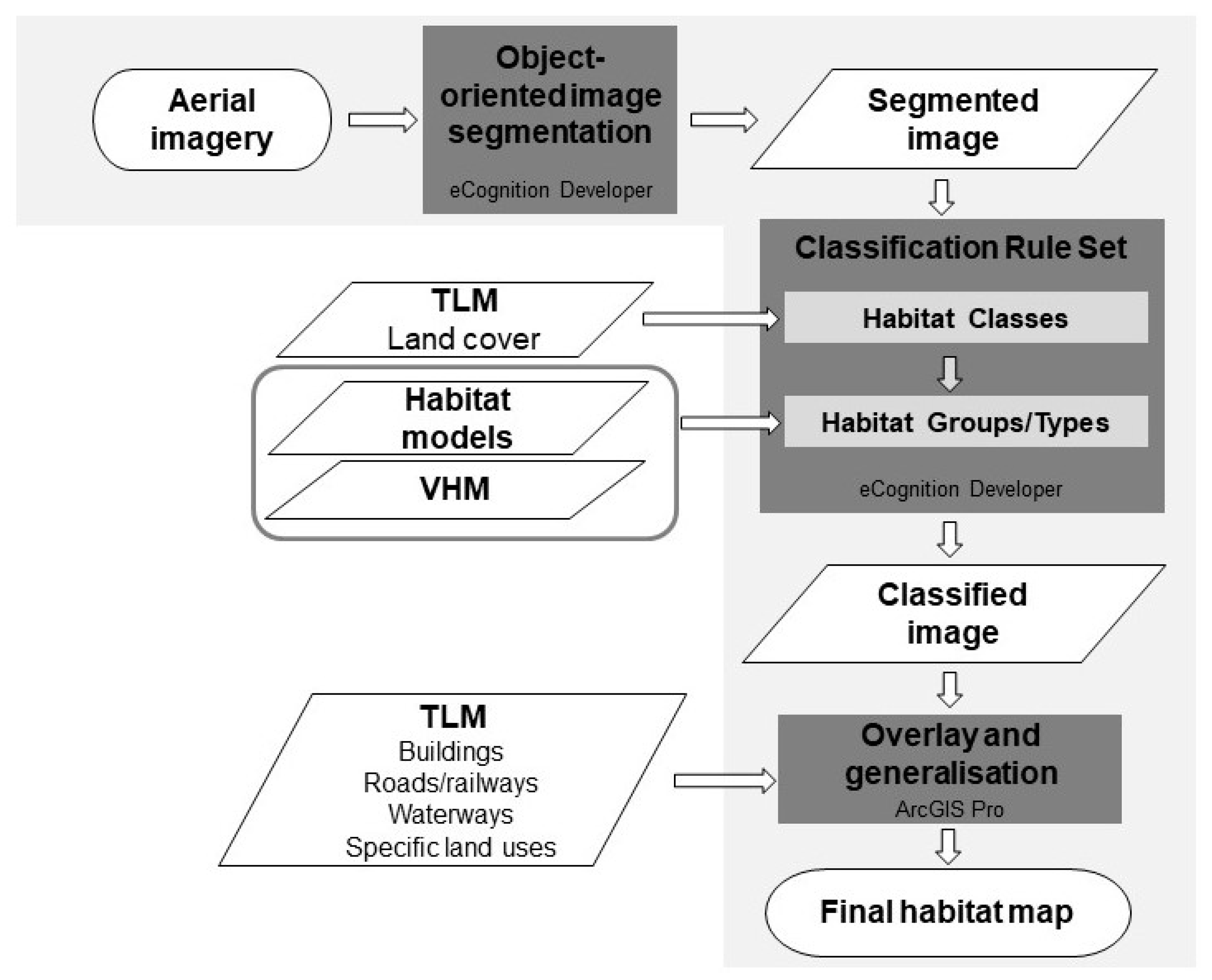
2.2. Overview Methodology
2.3. Imagery
2.4. Habitat Distribution Data
2.4.1. Swisstopo TLM
2.4.2. Habitat Distribution Models
2.4.3. Species Distribution Models
2.4.4. Classification Rules
2.5. Image Segmentation
2.6. Classification Process
2.7. Probability and Percentage Cover
2.8. Vector Update and Cleaning
2.9. Validation
2.9.1. Delarze et al. [21] Coarse Distribution Maps
2.9.2. Swiss Land Use Statistics
2.9.3. Aerial Image Interpretation
2.9.4. SwissFungi
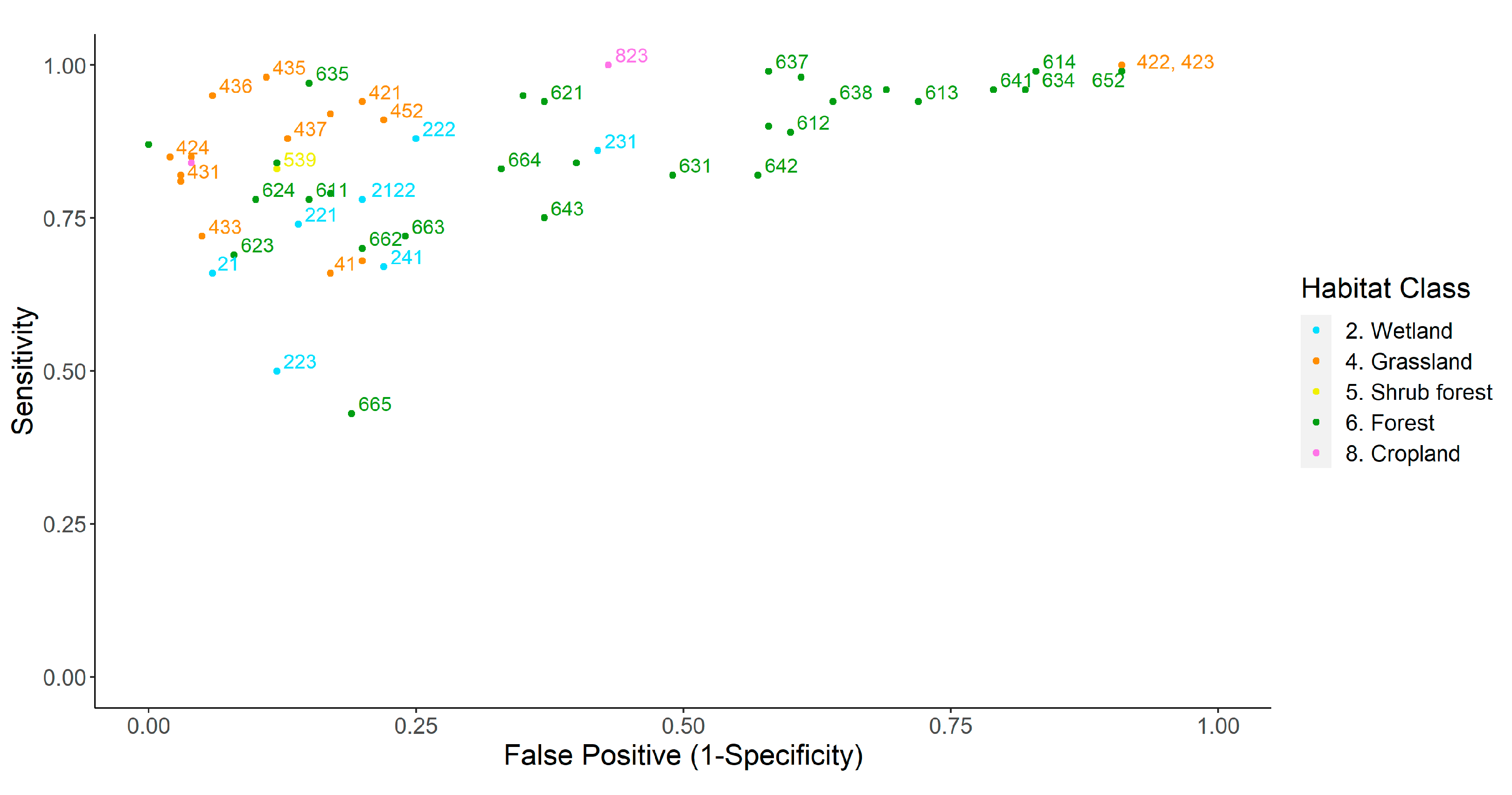
3. Results
Validation
4. Discussion and Conclusions
Supplementary Materials
Author Contributions
Funding
Data Availability Statement
Acknowledgments
Conflicts of Interest
References
- Edwards, P.J.; May, R.M.; Webb, N.R.P. Large Scale Ecology and Conservation Biology; Edwards, P.J., May, R.M., Webb, N.R., Eds.; Blackwell Scientific Publications: Oxford, UK, 1994; pp. viii–xi. [Google Scholar]
- Potschin, M.; Haines-Young, R. Ecosystem Services. Exploring a geographical perspective. Prog. Phys. Geogr. 2011, 35, 575–594. [Google Scholar] [CrossRef]
- Liquete, C.; Kleeschulte, S.; Dige, G.; Maes, J.; Grizzetti, B.; Olah, B.; Zulian, G. Mapping green infrastructure based on ecosystem services and ecological networks: A Pan-European case study. Environ. Sci. Policy 2015, 54, 268–280. [Google Scholar] [CrossRef]
- Gavish, Y.; O’Connell, J.; Marsh, C.J.; Tarantino, C.; Blonda, P.; Tomaselli, V.; Kunin, W.E. Comparing the performance of flat and hierarchical habitat/land-cover classification models in a natura 2000 site. ISPRS J. Photogramm. Remote Sens. 2018, 136, 1–12. [Google Scholar] [CrossRef]
- Swiss Federal Statistical Office. Die Bodennutzung in der Schweiz: Resultate der Arealstatistik 2018; Report nr. 002-1801; Federal Statistical Office: Neuchtatel, Switzerland, 2021; 36p. [Google Scholar]
- Copernicus Land Monitoring Service. Corine Land Cover, 2018 © European Union, European Environment Agency (EEA). Available online: https://land.copernicus.eu/pan-european/corine-land-cover/clc2018 (accessed on 11 November 2022).
- European Environmental Agency. An introduction to habitats. Available online: https://www.eea.europa.eu/themes/biodiversity/an-introduction-to-habitats. (accessed on 11 November 2022).
- Jin, S.; Homer, C.; Yang, L.; Danielson, P.; Dewitz, J.; Li, C.; Zhu, Z.; Xian, G.; Howard, D. Overall Methodology Design for the United States National Land Cover Database 2016 Products. Remote Sens. 2019, 11, 2971. [Google Scholar] [CrossRef] [Green Version]
- Marston, C.; Rowland, C.S.; O’Neil, A.W.; Morton, R.D. Land Cover Map 2021 (10m Classified Pixels, GB); NERC EDS Environmental Information Data Centre: lancashire, UK, 2022. [Google Scholar] [CrossRef]
- Buchhorn, M.; Lesiv, M.; Tsendbazar, N.-E.; Herold, M.; Bertels, L.; Smets, B. Copernicus Global Land Cover Layers—Collection 2. Remote Sens. 2020, 12, 1044. [Google Scholar] [CrossRef] [Green Version]
- Potapov, P.; Hansen, M.C.; Pickens, A.; Hernandez-Serna, A.; Tyukavina, A.; Turubanova, S.; Zalles, V.; Li, X.; Khan, A.; Stolle, F.; et al. The Global 2000-2020 Land Cover and Land Use Change Dataset Derived From the Landsat Archive: First Results. Front. Remote Sens. 2022, 3, 856903. [Google Scholar] [CrossRef]
- Corbane, C.; Lang, S.; Pipkins, K.; Alleaume, S.; Deshayes, M.; García Millán, V.E.; Strasser, T.; Vanden Borre, J.; Toon, S.; Michael, F. Remote sensing for mapping natural habitats and their conservation status—New opportunities and challenges. Int J Appl Earth Obs Geoinf 2015, 37, 7–16. [Google Scholar] [CrossRef]
- He, K.S.; Bradley, B.A.; Cord, A.F.; Rocchini, D.; Tuanmu, M.N.; Schmidtlein, S.; Turner, W.; Wegmann, M.; Pettorelli, N.; Nagendra, H.; et al. Will remote sensing shape the next generation of species distribution models? Remote Sens. Ecol. Conserv. 2015, 1, 4–18. [Google Scholar] [CrossRef] [Green Version]
- Kilcoyne, A.M.; Clement, M.; Moore, C.; Picton Phillipps, G.P.; Keane, R.; Woodget, A.; Potter, S.; Stefaniak, A.; Trippier, B. Living England: Satellite-based habitat calssification.Technical User Guide. Available online: http://nepubprod.appspot.com/publication/4918342350798848. (accessed on 11 November 2022).
- NatureScot. Habitat Map of Scotland. 2022. Available online: https://www.nature.scot/landscapes-and-habitats/habitat-map-scotland (accessed on 11 November 2022).
- Bell, G.; Neal, S.; Medcalf, K. Use of remote sensing to produce a habitat map of Norfolk. Ecol. Inform. 2015, 30, 293–299. [Google Scholar] [CrossRef]
- Sittaro, F.; Hutengs, C.; Semella, S.; Vohland, M. A Machine Learning Framework for the Classification of Natura 2000 Habitat Types at Large Spatial Scales Using MODIS Surface Reflectance Data. Remote Sens. 2022, 14, 823. [Google Scholar] [CrossRef]
- Kwong, I.H.Y.; Wong, F.K.K.; Fung, T.; Liu, E.K.Y.; Lee, R.H.; Ng, T.P.T. A Multi-Stage Approach Combining Very High-Resolution Satellite Image, GIS Database and Post-Classification Modification Rules for Habitat Mapping in Hong Kong. Remote Sens. 2022, 14, 67. [Google Scholar] [CrossRef]
- Horvath, P.; Halvorsen, R.; Stordal, F.; Tallaksen, L.M.; Tang, H.; Bryn, A. Distribution modelling of vegetation types based on area frame survey data. Appl. Veg. Sci. 2019, 22, 547–560. [Google Scholar] [CrossRef] [Green Version]
- Butler, L.; Sanderson, R.A. National-scale predictions of plant assemblages via community distribution models: Leveraging published data to guide future surveys. J. Appl. Ecol. 2022, 59, 1559–1571. [Google Scholar] [CrossRef]
- Delarze, R.; Gonseth, Y.; Eggenberg, S.; Vust, M. Lebensräume der Schweiz. Ökologie—Gefährdung—Kennarten, 3rd ed.; hep verlag ag: Bern, Switzlerland, 2015; 456p. [Google Scholar]
- Pasche, S.; Maire, A.-L.; Bourguignon, Y.; Martin, P.; Mombrial, F.; Prunier, P. Les milieux naturels genevois: Fiches descriptives 2016. Available online: https://www.patrimoine-vert-geneve.ch/. (accessed on 11 November 2022).
- OECD. OECD Environmental Performance Reviews: Switzerland 2017; OECD Environmental Performance Reviews; OECD Publishing: Paris, France. [CrossRef]
- European Environmental Agency. The European Environment—State and Outlook 2020: Knowledge for Transition to a Sustainable Europe; Publications Office of the EU: Copenhagen, Denmark, 2019; p. 496. [Google Scholar] [CrossRef]
- Delarze, R.; Eggenberg, S.; Steiger, P.; Bergamini, A.; Fivaz, F.; Gonseth, Y.; Guntern, J.; Hofer, G.; Sager, L.; Stucki, P. Rote Liste Lebensräume der Schweiz. Aktualisierte Kurzfassung Zum Technischen Bericht 2013 (Technical Report); Swiss Federal Office of the Environment: Bern, Switzerland, 2016; 33p. [Google Scholar]
- Swiss Federal Office of Topography swisstopo. swissTLM3D. Available online: https://www.swisstopo.admin.ch/en/geodata/landscape/tlm3d.html. (accessed on 11 November 2022).
- Swiss Federal Office of Topography swisstopo. Swissimage. Available online: https://www.swisstopo.admin.ch/en/geodata/images/ortho/swissimage10.html. (accessed on 11 November 2022).
- Ginzler, C.; Hobi, M.L. Countrywide stereo-image matching for updating digital surface models in the framework of the Swiss National Forest Inventory. Remote Sens. 2015, 7, 4343–4370. [Google Scholar] [CrossRef] [Green Version]
- Huber, N.; Ginzler, C.; Pazur, R.; Descombes, P.; Baltensweiler, A.; Ecker, K.; Meier, E.; Price, B. Countrywide classification of permanent grassland habitats at high spatial resolution. Remote Sens. Ecol. Conserv. 2022, 19. [Google Scholar] [CrossRef]
- Rüetschi, M.; Weber, D.; Koch, T.L.; Waser, L.T.; Small, D.; Ginzler, C. Countrywide mapping of shrub forest using multi-sensor data and bias correction techniques. Int. J Appl. Earth Obs. Geoinf. 2021, 105, 10. [Google Scholar] [CrossRef]
- Wüest, R.O.; Bergamini, A.; Bollmann, K.; Brändli, U.; Baltensweiler, A. Modellierte Verbreitungskarten für die häufigsten Gehölzarten der Schweiz. Schweizerische Zeitschrift für Forstwesen 2021, 172, 226–233. [Google Scholar] [CrossRef]
- Pazúr, R.; Huber, N.; Weber, D.; Ginzler, C.; Price, B. A national extent map of cropland and grassland for Switzerland based on Sentinel-2 data. Earth Syst. Sci. Data 2022, 14, 295–305. [Google Scholar] [CrossRef]
- Gross, A.; Blaser, S.; Senn-Irlet, B.J. SwissFungi Verbreitungskarte. Available online: https://www.wsl.ch/map_fungi. (accessed on 29 April 2021).
- Araújo, M.B.; New, M. Ensemble forecasting of species distributions. Trends Ecol. Evol. 2007, 22, 42–47. [Google Scholar] [CrossRef]
- Masek, J.G.; Vermote, E.F.; Saleous, N.; Wolfe, R.; Hall, F.G.; Huemmrich, F.; Gao, F.; Kutler, J.; Lim, T.K. LEDAPS Calibration, Reflectance, Atmospheric Correction Preprocessing Code, Version 2 (Model Product); Oak Ridge National Laboratory: Lancashire, UK, 2013. [CrossRef]
- Swiss Federal Office of Topography swisstopo, DHM25, 1994. Available online: https://www.swisstopo.admin.ch/en/geodata/height/dhm25.html. (accessed on 11 November 2021).
- Swiss Federal Office of Topography swisstopo. swissALTI3D. Available online: https://www.swisstopo.admin.ch/en/geodata/height/alti3d.html. (accessed on 11 November 2021).
- Waser, L.T.; Fischer, C.; Wang, Z.; Ginzler, C. Wall-to-wall forest mapping based on digital surface models from image-based point clouds and a NFI forest definition. Forests 2015, 6, 4510–4528. [Google Scholar] [CrossRef] [Green Version]
- Kubat, M.; Holte, R.C.; Matwin, S. Machine learning for the detection of oil spills in satellite radar images. Machine Learning 1998, 30, 195–215. [Google Scholar] [CrossRef] [Green Version]
- Welten, M.; Sutter, R. Verbreitungsatlas der Farn- und Blütenplfanzen der Schweiz; Birkhäuser: Basel, Switzerland, 1982; Band I: 716 p., Band II: 698 p. [Google Scholar]
- Vilpert, M.; Eggenberg, S.; Schiendorfer, L. Info Flora Jahresbericht/Rapport Annuel. Available online: https://www.infoflora.ch/en/assets/content/documents/Jahresbericht_IF_2021.pdf. (accessed on 11 November 2021).
- Moser, D.; Gygax, A.; Bäumler, B.; Wyler, N.; Raoul, P. Rote Liste der gefährdeten Farn- und Blütenpflanzen der Schweiz; Swiss Federal Office for the Environment: Bern, Switzerland, 2002; 118p. [Google Scholar]
- Price, B.; Huber, N.; Ginzler, C.; Pazúr, R.; Rüetschi., M. The Habitat Map of Switzerland v1. (dataset). EnviDat 2021. [Google Scholar] [CrossRef]
- Iosifescu Enescu, I.; Plattner, G.K.; Pernas, L.E.; Haas-Artho, D.; Bischof, S.; Lehning, M.; Steffen, K. The EnviDat concept for an institutional environmental data portal. Data Sci. J. 2018, 17, 28–45. [Google Scholar] [CrossRef] [Green Version]
- Treindl, A.; Brännhage, J.; Schlegel, M.; Vlcek, P.; Zengerer, V.; Blaser, S.; Gross, A. Erstes Jahr eines Grossprojekts für den Schweizer Pilzschutz. Ein Rück- und Ausblick zur Feldkampagne für die neue Rote Liste der Grosspilze. Schweizerische Zeitschrift für Pilzkunde 2022, 100, 24–26. Available online: https://www.dora.lib4ri.ch/wsl/islandora/object/wsl:30058 (accessed on 28 November 2022).
- Swiss Federal Office for the Environment. Bundesinventar der Amphibienlaichgebiete von nationaler Bedeutung. Available online: www.bafu.admin.ch/amphibienlaichgebiete. (accessed on 11 November 2021).
- Bock, M.; Xofis, P.; Mitchley, J.; Rossner, G.; Wissen, W. Object-oriented methods for habitat mapping at multiple scales — case studies from northern Germany and wye Downs, UK. J. Nat. Conserv. 2005, 13, 75–89. [Google Scholar] [CrossRef]
- Griffiths, P.; Nendel, C.; Hostert, P. Intra-annual reflectance composites from Sentinel-2 and Landsat for national-scale crop and land cover mapping. Remote Sens. Environ. 2018, 220, 135–151. [Google Scholar] [CrossRef]
- Janowski, L.; Trzcinska, K.; Tegowski, J.; Kruss, A.; Rucinska-Zjadacz, M.; Pocwiardowski, P. Nearshore Benthic Habitat Mapping Based on Multi-Frequency, Multibeam Echosounder Data Using a Combined Object-Based Approach: A Case Study from the Rowy Site in the Southern Baltic Sea. Remote Sens. 2018, 10, 1983. [Google Scholar] [CrossRef]
- Praticò, S.; Solano, F.; Di Fazio, S.; Modica, G. Machine Learning Classification of Mediterranean Forest Habitats in Google Earth Engine Based on Seasonal Sentinel-2 Time-Series and Input Image Composition Optimisation. Remote Sens. 2021, 13, 586. [Google Scholar] [CrossRef]
- Tarantino, C.; Forte, L.; Blonda, P.; Vicario, S.; Tomaselli, V.; Beierkuhnlein, C.; Adamo, M. Intra-Annual Sentinel-2 Time-Series Supporting Grassland Habitat Discrimination. Remote Sens. 2021, 13, 277. [Google Scholar] [CrossRef]
- Tillé, Y.; Ecker, K. Complex national sampling design for long-term monitoring of protected dry grasslands in Switzerland. Environ Ecol Stat. 2014, 21, 453–476. [Google Scholar] [CrossRef] [Green Version]
- Breiner, F.T.; Guisan, A.; Bergamini, A.; Nobis, M.P. Overcoming limitations of modelling rare species by using ensembles of small models. Methods Ecol. Evol. 2015, 6, 1210–1218. [Google Scholar] [CrossRef]
- Swiss Federal Office of Topography Swisstopo. LiDAR Data Acquisition. Available online: https://www.swisstopo.admin.ch/en/knowledge-facts/geoinformation/lidar-data.html. (accessed on 11 November 2021).
- Degerickx, J.; Hermy, M.; Somers, B. Mapping Functional Urban Green Types Using High Resolution Remote Sensing Data. Sustainability 2020, 12, 2144. [Google Scholar] [CrossRef]


| TypoCH | Class | Group | TypoCH Name | Source (Method) | Validation Source |
|---|---|---|---|---|---|
| 1 | 1 | - | Non-marine water bodies | 1 | SLUS |
| 1.1 | 1 | 11 | Standing fresh water | 1 | SLUS |
| 1.2 | 1 | 12 | Running water | 1 | SLUS |
| 1.3 | 1 | 13 | Springs | 9 | NA |
| 1.4 | 1 | 14 | Underground waters | 9 | NA |
| 2 | 2 | - | Banks, shores and wetlands | 1 | [21,29] |
| 2.0 | 2 | 20 | Artificial banks | 1 | NA |
| 2.1 | 2 | 21 | Bank and shore vegetation | 1 | [21,29] |
| 2.2 | 2 | 22 | Fens and transition mires | 2 | [21,29] |
| 2.3 | 2 | 23 | Wet meadows | 2 | [21,29] |
| 2.4 | 2 | 24 | Raised bogs | 2 | [21,29] |
| 2.5 | 2 | 25 | Temporarily flooded annual vegetation | 9 | NA |
| 3 | 3 | - | Glaciers, rocks, screes and gravel | 1 | SLUS |
| 3.1 | 3 | 31 | Glaciers, permanent ice and snow | 1 | SLUS |
| 3.2 | 3 | 32 | Alluvial deposits and moraines | 1 | SLUS, AII |
| 3.3 | 3 | 33 | Screes | 1 | SLUS, AII |
| 3.4 | 3 | 34 | Cliffs and exposed rocks | 1 | SLUS, AII |
| 3.5 | 3 | 35 | Caves | 9 | NA |
| 4 | 4 | 4 | Grasslands | 2 | [21,29] |
| 4.0 | 4 | 40 | Re-seeded and heavily fertilised grasslands (re-seeded grasslands) | 2 | [21,29] |
| 4.1 | 4 | 41 | Pioneer vegetation on rocky surfaces | 4 | SLUS, [21] |
| 4.2 | 4 | 42 | Dry grasslands | 2 | [21,29] |
| 4.3 | 4 | 43 | Nutrient-poor alpine and subalpine grasslands (alpine/subalpine grasslands) | 2 | [21,29] |
| 4.4 | 4 | 44 | Snowbed communities | 2 | NV |
| 4.5 | 4 | 45 | Nutrient-rich pastures and meadows | 2 | [21,29] |
| 4.6 | 4 | 46 | Fallow grasslands | 9 | NA |
| 5 | 5 | - | Woodland edges, tall herb communities, shrubs | 1 | [21,30], AII |
| 5.1 | 5 | 51 | Herbaceous fringes | 9 | NA |
| 5.2 | 5 | 52 | Forest clearings | 4 | AII |
| 5.3 | 5 | 53 | Shrubs, bushes, hedges | 1 | [21,30], AII |
| 5.4 | 5 | 54 | Dry dwarf shrub heaths | 2 | [30], AII |
| 6 | 6 | - | Forests | 1 | [21,31,33] |
| 6.0 | 6 | 60 | Plantations and trees outside forest | 4 | [21,31,33] |
| 6.1 | 6 | 61 | Swamp forests | 3 | [21,31,33] |
| 6.2 | 6 | 62 | Beech forests | 3 | [21,31,33] |
| 6.3 | 6 | 63 | Other deciduous forests | 3 | [21,31,33] |
| 6.4 | 6 | 64 | Thermophilic pine forests | 3 | [21,31,33] |
| 6.5 | 6 | 65 | Bog forests | 3 | [21,31,33] |
| 6.6 | 6 | 66 | High-altitude coniferous forests | 3 | [21,31,33] |
| 7 | 7 | - | Pioneer vegetation of disturbed areas (ruderal vegetation) | 4 | NV |
| 7.1 | 7 | 71 | Trampled and ruderal areas | 4 | NV |
| 7.2 | 7 | 72 | Anthropogenic rocky habitats | 9 | NA |
| 8 | 8 | - | Plantations and cropland | 2 | [32], SLUS |
| 8.1 | 8 | 81 | Tree nurseries, orchards, vineyards | 1 | [32], SLUS |
| 8.2 | 8 | 82 | Cropland | 2 | [21,32], SLUS |
| 9 | 9 | - | Built habitats | 1 | SLUS |
| 9.1 | 9 | 91 | Dumps | 9 | NA |
| 9.2 | 9 | 92 | Buildings | 1 | SLUS |
| 9.3 | 9 | 93 | Transport routes | 1 | SLUS |
| 9.4 | 9 | 94 | Sealed sports grounds, car parks, etc. | 1 | SLUS |
| TLM Dataset | Original Object Code | Description of TLM Class | TypoCH | TypoCH Name |
|---|---|---|---|---|
| TLM landcover | 1 * | Rock surfaces | 3.4 | Cliffs and exposed rocks |
| TLM landcover | 2 * | Loose rock | 3.3 | Screes |
| TLM landcover | 3 * | Boulders | 3.3 | Screes |
| TLM landcover | 4 * | Boulders, loose | 3.3 | Screes |
| TLM landcover | 5 | Running water | 1.2 | Running water |
| TLM landcover | 6 | Shrub forest | 5.3 | Shrubs, bushes, hedges |
| TLM landcover | 7 * | Loose rock | 3.3 | Screes |
| TLM landcover | 8 * | Loose rock, loose | 3.3 | Screes |
| TLM landcover | 9 | Glaciers | 3.1 | Glaciers, permanent ice and snow |
| TLM landcover | 10 | Standing water | 1.1 | Standing fresh water |
| TLM landcover | 11 * | Wetlands | 2 | Wetlands |
| TLM landcover | 12 * | Forest | 6 | Forests |
| TLM landcover | 13 * | Open forest | 6 | Forests |
| TLM landcover | 14 * | Wooded area with VHM > 3m, VHM < 3m | 6.0.0, 5.3 | Trees outside forest, shrubs, bushes, hedges |
| TLM roads and paths | all | with surface type (‘Belagsart’) = 100 | 9.3.2 | Sealed roads |
| TLM roads and paths | all | with surface type (‘Belagsart’) = 200 | 9.3.3 | Unsurfaced track, lane |
| TLM railways | all | Railways | 9.3.4 | Railway |
| TLM building footprints | all excluding 16 | Buildings | 9.2 | Building |
| TLM sports facilities | 0 (with mean NDVI < 0.1) | Sports field | 9.4 | Sealed sports ground, car park, etc. |
| TLM sports facilities | 1 (with mean NDVI > 0.1) | Sports field | 4.0.2 | Artificial lawns; sport and urban areas |
| TLM dams and weirs | 0 | Dam wall | 9 | Built habitats |
| TLM dams and weirs | 1 | Dam | 9 | Built habitats |
| TLM dams and weirs | 2 | Water basins | 1.1 | Standing water |
| TLM dams and weirs | 3 | Weir | 9 | Built habitats |
| TLM transport facilities | 2 | Grass piste | 4.0.2 | Artificial lawns; sport and urban areas |
| TLM transport facilities | 3 | Hard surface piste | 9.3.2 | Sealed roads |
| TLM transport facilities | 4 | Platforms | 9.3 | Transport routes |
| TLM transport facilities | 5 | Tarmac grass | 4.0.2 | Artificial lawns; sport and urban areas |
| TLM transport facilities | 6 | Tarmac hard surface | 9.3.2 | Sealed roads |
| TLM transport facilities | 7 | Lock (canal) | 1.2 | Running water |
| TLM special use areas | 3 | Tree nursery | 8.1 | Tree nurseries, orchards, vineyards |
| TLM special use areas | 9 | Waste incineration area | 9 | Built habitats |
| TLM special use areas | 15 | Orchards | 8.1 | Tree nurseries, orchards, vineyards |
| TLM special use areas | 17 | Vineyards | 8.1.6 | Vineyards |
| TLM special use areas | 18 | Allotment gardens | 8.2.3 | Root crops, gardens |
| TLM special use areas | 23 | Substation area | 9.2 | Building |
| TLM special use areas | 5 | Public car park | 9.4 | Sealed sports ground, car park, etc. |
| TLM special use areas | All others not included | |||
| TLM traffic areas | 10 | Private car park | 9.4 | Sealed sports ground, car park, etc. |
| TLM traffic areas | All others not included | |||
| TLM recreation areas | Not included |
| TypoCH | Classification Rule |
|---|---|
| 2.1 Banks and shore vegetation | TLM landcover running or standing water with mean NDVI (aerial imagery) > 0.1 and 95th percentile growing season NDVI (Sentinel 2) > 0.1 |
| 3.2.1 River gravel banks | TLM landcover loose rock surfaces, boulders, gravel or loose gravel bordering running water |
| 3.2.2 Moraines | TLM landcover loose rock surfaces, boulders, gravel or loose gravel bordering TLM landcover glaciers |
| 4 Grassland | Non-classified areas (non-tree or shrub) within the settlement boundary: 95th percentile of growing season NDVI (Sentinel 2) > 0.3 |
| 4.1 Pioneer vegetation on rocky surfaces | TLM landcover rock surfaces with median growing season NDVI (Sentinel 2) > 0.2 and < 0.45 |
| 5.2 Forest clearings | TLM landcover forest or open forest with mean VHM 2012 > 3m and mean VHM 2019 < 3 m |
| 5.3.0 Hedges and shrubs outside of shrub forest | No TLM landcover classification with median VHM 2019 > 1.5m and median VHM2019 < 3 m, and mean NDVI (aerial imagery) > 0.2 TLM landcover other wooded areas with mean VHM < 3m |
| 6.0.0 Trees outside forest | No TLM landcover classification with median VHM 2019 > 3 m and mean NDVI (aerial imagery) > 0.2 |
| 7.1 Trampled and ruderal areas | Within the settlement boundary: 95th percentile of growing season NDVI (Sentinel 2) < 0.3 Outside the settlement boundary: No classification with median growing season NDVI (Sentinel 2) < 0.2 |
| TypoCH | Name | Latin Name | Area |
|---|---|---|---|
| 1 | Non-marine water bodies total | 4% | |
| 1.1 | Standing fresh water | 86% (143,621 ha) | |
| 1.2 | Running water | 14% (22,580 ha) | |
| 2 | Banks, shores and wetlands total | 1.5% | |
| 2.1 | Bank and shore vegetation | 7% (3100 ha) | |
| 2.1 | Bank and shore vegetation | 5% (2954 ha) | |
| 2.1.2.2 | Riverbank and terrestrial reeds | Phalaridion arundinaceae | 2% (1046 ha) |
| 2.2 | Fens and transition mire | 40% (25,239 ha) | |
| 2.2.1 | Large sedge communities | Magnocaricion elatae, Cladietum marisci | 3% (1567 ha) |
| 2.2.2 | Acidic fens | Caricion fuscae | 9% (5915 ha) |
| 2.2.3 | Calcareous fens | Caricion davallianae | 28% (17,757 ha) |
| 2.3 | Wet meadows total | 53% (32,574 ha) | |
| 2.3.1 | Purple moorgrass meadows | Molinion caerulea | 2% (1061 ha) |
| 2.3.2/3 | Nutrient-rich humid meadows (marsh marigold meadow) | Calthion palustris, Filipendulion ulmariae | 49% (30,526 ha) |
| 2.4 | Raised bogs total | 2% (987 ha) | |
| 2.4.1 | Bog hummocks, ridges and lawns | Sphagnion magellanici | 2% (987 ha) |
| 3 | Glaciers, rocks, screes and gravel total | 14% | |
| 3 | Gravel (not assigned to a group) | 1% (8460 ha) | |
| 3.1 | Glaciers, permanent ice and snow | 16% (92,758 ha) | |
| 3.2 | Alluvial deposits and moraines | 4% (24,672 ha) | |
| 3.2.1 | River gravel banks | 1% (8764 ha) | |
| 3.2.2 | Moraines | 3% (15,908 ha) | |
| 3.3 | Screes | 45% (262,491 ha) | |
| 3.4 | Cliffs and exposed rocks | 34% (196,354 ha) | |
| 4 | Grasslands total | 32.5% | |
| 4 | Grasslands | 8% (109,488 ha) | |
| 4.0 | Re-seeded grasslands | 2% (32,536 ha) | |
| 4.0 | Re-seeded and heavily fertilised grasslands | 2% (30,209 ha) | |
| 4.0.2 | Artificial lawns; sports, urban areas | <1% (2327 ha) | |
| 4.1 | Pioneer vegetation on rocky surfaces | 5% (66,667 ha) | |
| 4.2 | Thermophilic dry grasslands | 4% (48,254 ha) | |
| 4.2.1 | Subcontinental steppe grasslands | Stipo-Poion carniolicae, Stipo-Poion xerophilae, Cirsio-Brachypodion | <1% (4534 ha) |
| 4.2.2 | Sub-Atlantic very dry calcareous grasslands | Xerobromion | <1% (38 ha) |
| 4.2.3 | Insubrian Mesobromion grasslands | Diplachnion serotinae | <1% (1ha) |
| 4.2.4 | Middle-European semi-dry calcareous grasslands | Mesobromion | 3% (43,681 ha) |
| 4.3 | Unfertilised mountain grasslands and pastures | 32% (429,334) | |
| 4.3.1 | Blue moorgrass–evergreen sedge slopes | Seslerion caeruleae | 4% (55,961 ha) |
| 4.3.2/4 | Cushion sedge meadows | Caricion firmae, Elynion myosuroides | 2% (24,286 ha) |
| 4.3.3 | Northern rust sedge grasslands | Caricion ferrugineae | 7% (90,336 ha) |
| 4.3.5 | Nardion grassland | Nardion strictae | 12% (161,354 ha) |
| 4.3.6 | Subalpine thermophilic siliceous grasslands | Festucion variae | 3% (38,270 ha) |
| 4.3.7 | Crooked sedge swards | Caricion curvulae | 4% (59,127 ha) |
| 4.4 | Snowbed communities | 2% (28,133 ha) | |
| 4.5 | Fertilised grasslands | 47% (630,712 ha) | |
| 4.5.1 | Medio-European lowland hay meadows | Arrhenatherion elatioris | 25% (336,271 ha) |
| 4.5.2 | Mountain and subalpine hay meadows | Polygono-Trisetion flavescentis | 3% (42,626 ha) |
| 4.5.3 | Mesophile pastures | Cynosurion cristate | 13% (175,973 ha) |
| 4.5.4 | Rough hawkbit pastures | Poion alpinae | 6% (75,842 ha) |
| 5 | Woodland edges, tall herbs communities, shrubs total | 3% | |
| 5.2 | Forest clearings | 16% (18,511 ha) | |
| 5.3 | Shrubs, bushes, hedges | 42% (49,814 ha) | |
| 5.3 | Shrubs, bushes, hedges | 9% (11,293 ha) | |
| 5.3.0 | Hedges and hedgerows | 8% (9220 ha) | |
| 5.3.9 | Alpine green alder shrub heaths | Alnenion viridis, Alnenion viridis | 25% (29,301 ha) |
| 5.4 | Dry dwarf shrub heaths | 42% (50,554 ha) | |
| 6 | Forests total | 32% | |
| 6 | Forests | 1% (10,400 ha) | |
| 6.0 | Plantations and trees outside forest | 4% (55,786 ha) | |
| 6.1 | Swamp forests total | <1% (5320 ha) | |
| 6.1 | Swamp forests | <1% (1031 ha) | |
| 6.1.1 | Alder swamp forests | Alnion glutinosae | <1% (3409 ha) |
| 6.1.2 | White willow gallery forests | Salicion albae | <1% (601 ha) |
| 6.1.3 | Grey alder gallery forests | Alnion incanae | <1% (166 ha) |
| 6.1.4 | Medio-European stream ash–alder woods | Fraxinion excelsioris | <1% (113 ha) |
| 6.2 | Beech forests total | 51% (669,671 ha) | |
| 6.2 | Beech forests | 9% (115,447 ha) | |
| 6.2.1 | Beech forests with orchids | Cephalanthero-Fagenion | 4% (51,940 ha) |
| 6.2.2 | Woodrush beech forests | Luzulo-Fagenion | 1% (14,055 ha) |
| 6.2.3 | Neutrophilic beech forests | Galio odorati-Fagenion | 14% (187,977 ha) |
| 6.2.4 | Bittercress beech forests | Lonicero alpigenae-Fagenion | 9% (116,126 ha) |
| 6.2.5 | Asperulo-Fagetum beech forests | Abieti-Fagonion | 14% (184,126 ha) |
| 6.3 | Other deciduous forests total | 8% (103,968 ha) | |
| 6.3 | Other deciduous forests | <1% (4940 ha) | |
| 6.3.1 | Ravine sycamore–maple forests | Lunario-Acerion | <1% (2744 ha) |
| 6.3.2 | Thermophilic alpine and peri- alpine mixed lime forests | Tilion platyphylli | 1% (8179 ha) |
| 6.3.3 | Oak–hornbeam forests | Carpinion betuli | 1% (11,448 ha) |
| 6.3.4 | Downy oak forest | Quercion pubescenti-petraeae | 1% (8504 ha) |
| 6.3.5 | Quercus pubescens woods | Orno-Ostryon | <1% (1818 ha) |
| 6.3.6 | Acidophilous oak forests | Quericion robori-petraeae | <1% (2424 ha) |
| 6.3.7 | Insubrian acidophilous oak and chestnut forests | Castaneo-Quercetum | 5% (59,991 ha) |
| 6.3.8 | Deciduous forest with evergreen undergrowth | <1% (124 ha) | |
| 6.3.9 | Black locust plantations | Balloto nigrae-Robinion | <1% (3805 ha) |
| 6.4 | Thermophilic pine forests total | 3% (24,545 ha) | |
| 6.4 | Thermophilic pine forests | 1% (6718 ha) | |
| 6.4 | Thermophilic pine forests | 1% (6718 ha) | |
| 6.4.1 | Purple moor grass–Scots pine forests | Molinio-Pinion | <1% (156 ha) |
| 6.4.2 | Spring heath–Scots pine forests | Erico-Pinion sylvestris | 1% (14,642 ha) |
| 6.4.3 | Inner-alpine restharrow steppe forests | Ononido-Pinion | <1% (3029 ha) |
| 6.5 | Bog forests total | <1% (3512 ha) | |
| 6.5 | Bog forests | <1% (2278 ha) | |
| 6.5.1 | Sphagnum birch forests | Betulion pubescentis | <1% (196 ha) |
| 6.5.2 | Mountain pine bog forests | Ledo-Pinion | <1% (1 ha) |
| 6.5.3 | Peatmoss subalpine and sphagnum spruce forests | Sphagno girgensohnii-Piceetum | <1% (1037 ha) |
| 6.6 | High-altitude coniferous forests total | 34% (441,186 ha) | |
| 6.6 | High-altitude coniferous forests | 6% (75,015 ha) | |
| 6.6.1 | Fir forests | Abieti-Piceion | 3% (39,422 ha) |
| 6.6.2 | Spruce forests | Vaccinio-Piceion | 9% (122,679 ha) |
| 6.6.3 | Larch–cembran pine forests | Larici-Pinetum cembrae | 7% (91,571 ha) |
| 6.6.4 | Limestone larch forests | Junipero-Laricetum | 3% (34,852 ha) |
| 6.6.5 | Mountain pine forests | Erico-Pinion mugo | 6% (77,647 ha) |
| 7 | Pioneer vegetation of disturbed areas (ruderal vegetation) total | 1% | |
| 7.1 | Trampled and ruderal areas | 100% (38,920 ha) | |
| 8 | Plantations and cropland total | 9% | |
| 8.1 | Tree nurseries, orchards, vineyards total | 6% (23,093 ha) | |
| 8.1 | Tree nurseries, orchards, etc. | 2% (8432 ha) | |
| 8.1.6 | Vineyards | 4% (14,661 ha) | |
| 8.2 | Cropland total | 93% (345,849 ha) | |
| 8.2 | Cropland | 93% (344,601 ha) | |
| 8.2.3 | Gardens | <1% (1248 ha) | |
| 9 | Built habitats total | 3% | |
| 9.2 | Buildings | 40% (51,994 ha) | |
| 9.3 | Transport routes total | 58% (74,824ha) | |
| 9.3 | Transport routes | <1% (139 ha) | |
| 9.3.2 | Sealed roads | 40% (51,994 ha) | |
| 9.3.3 | Unsurfaced roads, tracks, lanes | 15% (19,149 ha) | |
| 9.3.4 | Railway | 3% (3542 ha) | |
| 9.4 | Sealed sports grounds, car parks, etc. | 2% (2830 ha) |
| TypoCH | Name | Percent Match | Swiss Land Use Statistics Classes |
|---|---|---|---|
| 1 | Non-marine water bodies | ||
| 1.1 | Standing fresh water | 0.99 | Standing water (61) |
| 1.2 | Running water | 0.72 | Running water (62) |
| 2 | Banks, shores and wetlands | ||
| 2.1 | Bank and shore vegetation | 0.86 | Standing water (61), Running water (62), Wetlands (67) |
| 2.x | Wetlands | 0.82 | Meadows (42), Alpine meadows (45), Favourable alpine pastures (46), Wetlands (67) |
| 3 | Glaciers, rocks, screes and gravel | ||
| 3.1 | Glaciers, permanent ice and snow | 0.97 | Glaciers and permanent snow (72) |
| 3.2.1 | River gravel banks | 0.87 | Running water (62), Gravel, sand (70) |
| 3.2.2 | Moraines | 0.99 | Rock surfaces (69), Scree, gravel, sand (70), Glaciers and permanent snow (72) |
| 3.3 | Screes | 0.80 | Rock surfaces (69), Scree, gravel, sand (70) |
| 3.4 | Cliffs and exposed rocks | 0.79 | Rock surfaces (69), Scree, gravel, sand (70) |
| 4 | Grasslands | ||
| 4.1 | Pioneer vegetation on rocky surfaces | 0.92 | Unproductive grass and shrubs (65), Rocks (69) |
| 4.x | All other grasslands | 0.90 | Building surrounds (2,4,6,8,10,12,14), Green road/airport environs (16, 18, 19, 23), Construction sites (29), Unexploited urban areas (30), Recreation areas (31–36), Arable land, pastures, meadows (41–49), Unproductive grass and shrubs (65) |
| 5 | Woodland edges, tall herb communities, shrubs | ||
| 5.2 | Forest clearings | 0.71 | Felling areas (53), Damaged forest areas (54), Open forest (55, 56) |
| 5.3, 5.4 | Shrubs, bushes, hedges; Dry dwarf shrub heaths | 0.77 | Brush alpine pastures (47), Brush forest (57), Scrub vegetation (64), Unproductive grass and shrubs (65) |
| 6 | Forests | ||
| 6.0 | Plantations and trees outside forest | 0.66 | Building surrounds (2,4,6,8,10,12,14), Green road environs (18), Recreation areas (31, 33, 34, 36), Field fruit trees (38), Woods (58–60) |
| 6.x | All other forests | 0.93 | Wooded areas (50–60) |
| 8 | Plantations and cropland | ||
| 8.1 | Tree nurseries, orchards, vineyards | 0.92 | Orchards (37), Fruit trees (38), Vineyards (39), Tree nurseries (40) |
| 8.1.6 | Vineyards | 0.97 | Vineyards (39) |
| 8.2 | Cropland | 0.88 | Cropland (41) |
| 8.2.3 | Gardens | 0.95 | Garden allotments (35) |
| 9 | Built habitats | ||
| 9.2 | Buildings | 0.85 | Buildings (1,3,5,7,9,11,13) |
| 9.3 | Transport routes | 0.97 | Car parks (19), Railway areas (20) |
| 9.3.2 | Sealed roads | 0.94 | Building surrounds (2,4,6,8,10,12,14), Motorways (15), Roads and paths (17), Carparks (19), Airports (22) |
| 9.3.3 | Unsurfaced roads, tracks, lanes | 0.63 | Building surrounds (2,4,6,8,10,12,14), Roads and paths (17,18), Car parks (19, 31), Building sites (28,29), |
| 9.3.4 | Railway | 0.93 | Railway areas (20,21) |
| 9.4 | Sealed sports grounds, car parks, etc. | 0.96 | Building surrounds (2,4,8,10,12,14), Car parks (19, 31), Building sites (29,30), Sports grounds (32) |
| TypoCH | Name | Sensitivity | Specificity | G-Mean |
|---|---|---|---|---|
| Aerial Image Interpretation | ||||
| 4 | Grassland | 0.95 | 0.91 | 0.9 |
| 6 | Forests | 0.96 | 0.94 | 0.9 |
| 3.1 | Glaciers, permanent ice and snow | 0.85 | 0.99 | 0.9 |
| 3.2 | Alluvial deposits and moraines | 0.31 | 0.99 | 0.5 |
| 3.3 | Screes | 0.69 | 0.96 | 0.8 |
| 3.4 | Cliffs and exposed rocks | 0.69 | 0.96 | 0.8 |
| 4.1 | Pioneer vegetation on rocky surfaces | 0.54 | 0.95 | 0.7 |
| 5.2 | Forest clearings | 0.03 | 0.99 | 0.2 |
| 5.3 | Shrubs, bushes, hedges | 0.64 | 0.99 | 0.8 |
| 5.4 | Dry dwarf shrub heaths | 0.38 | 0.99 | 0.6 |
| SwissFungi forest data | ||||
| 6.1 | Swamp forests | 0.29 | 0.99 | 0.54 |
| 6.2 | Beech forests | 0.94 | 0.51 | 0.69 |
| 6.3 | Other deciduous forests | 0.76 | 0.93 | 0.84 |
| 6.4 | Thermophilic pine forests | 0.42 | 0.99 | 0.64 |
| 6.5 | Bog forests | 0.52 | 0.99 | 0.72 |
| 6.6 | High-altitude coniferous forests | 0.45 | 0.98 | 0.67 |
Disclaimer/Publisher’s Note: The statements, opinions and data contained in all publications are solely those of the individual author(s) and contributor(s) and not of MDPI and/or the editor(s). MDPI and/or the editor(s) disclaim responsibility for any injury to people or property resulting from any ideas, methods, instructions or products referred to in the content. |
© 2023 by the authors. Licensee MDPI, Basel, Switzerland. This article is an open access article distributed under the terms and conditions of the Creative Commons Attribution (CC BY) license (https://creativecommons.org/licenses/by/4.0/).
Share and Cite
Price, B.; Huber, N.; Nussbaumer, A.; Ginzler, C. The Habitat Map of Switzerland: A Remote Sensing, Composite Approach for a High Spatial and Thematic Resolution Product. Remote Sens. 2023, 15, 643. https://doi.org/10.3390/rs15030643
Price B, Huber N, Nussbaumer A, Ginzler C. The Habitat Map of Switzerland: A Remote Sensing, Composite Approach for a High Spatial and Thematic Resolution Product. Remote Sensing. 2023; 15(3):643. https://doi.org/10.3390/rs15030643
Chicago/Turabian StylePrice, Bronwyn, Nica Huber, Anita Nussbaumer, and Christian Ginzler. 2023. "The Habitat Map of Switzerland: A Remote Sensing, Composite Approach for a High Spatial and Thematic Resolution Product" Remote Sensing 15, no. 3: 643. https://doi.org/10.3390/rs15030643