
Comparison and Assessment of Data Sources with Different Spatial and Temporal Resolution for Efficiency Orchard Mapping: Case Studies in Five Grape-Growing Regions

 ,
,  ,
,  , and
, and
Abstract
:1. Introduction
2. Study Area and Data
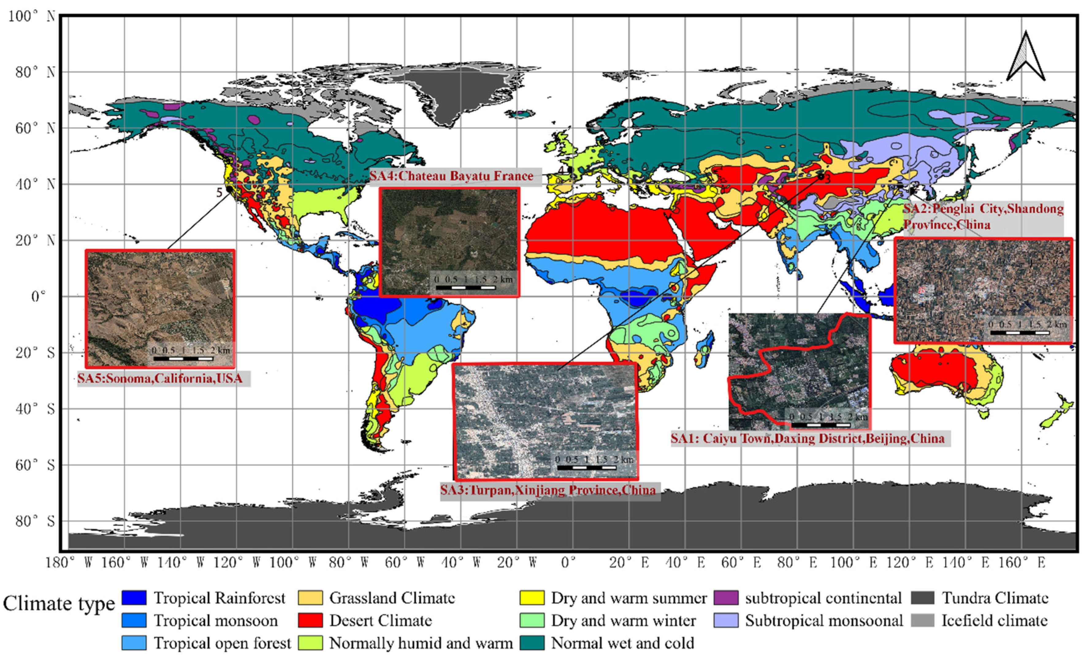
2.1. Study Area
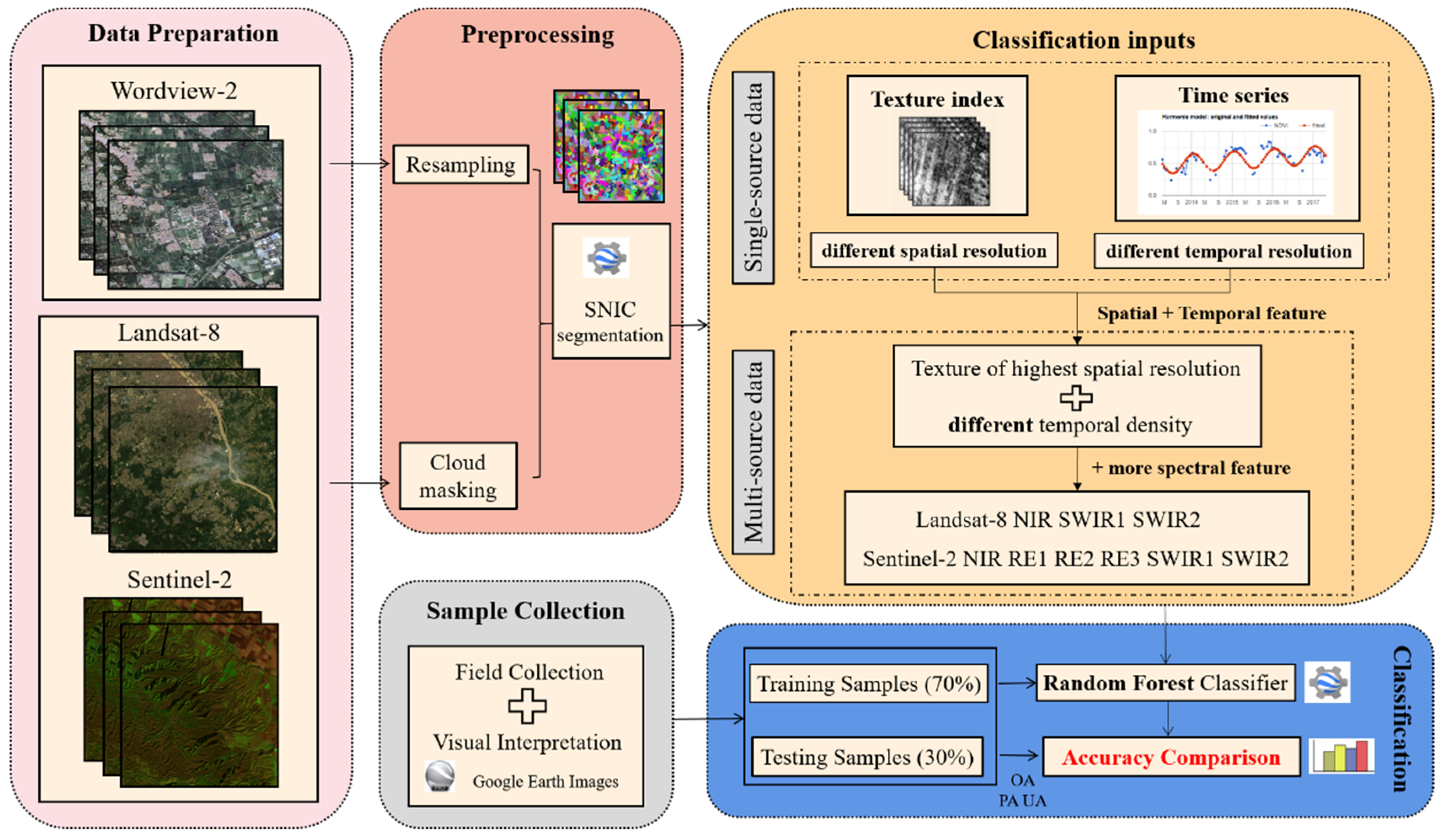
2.2. Data
2.2.1. VHR Images
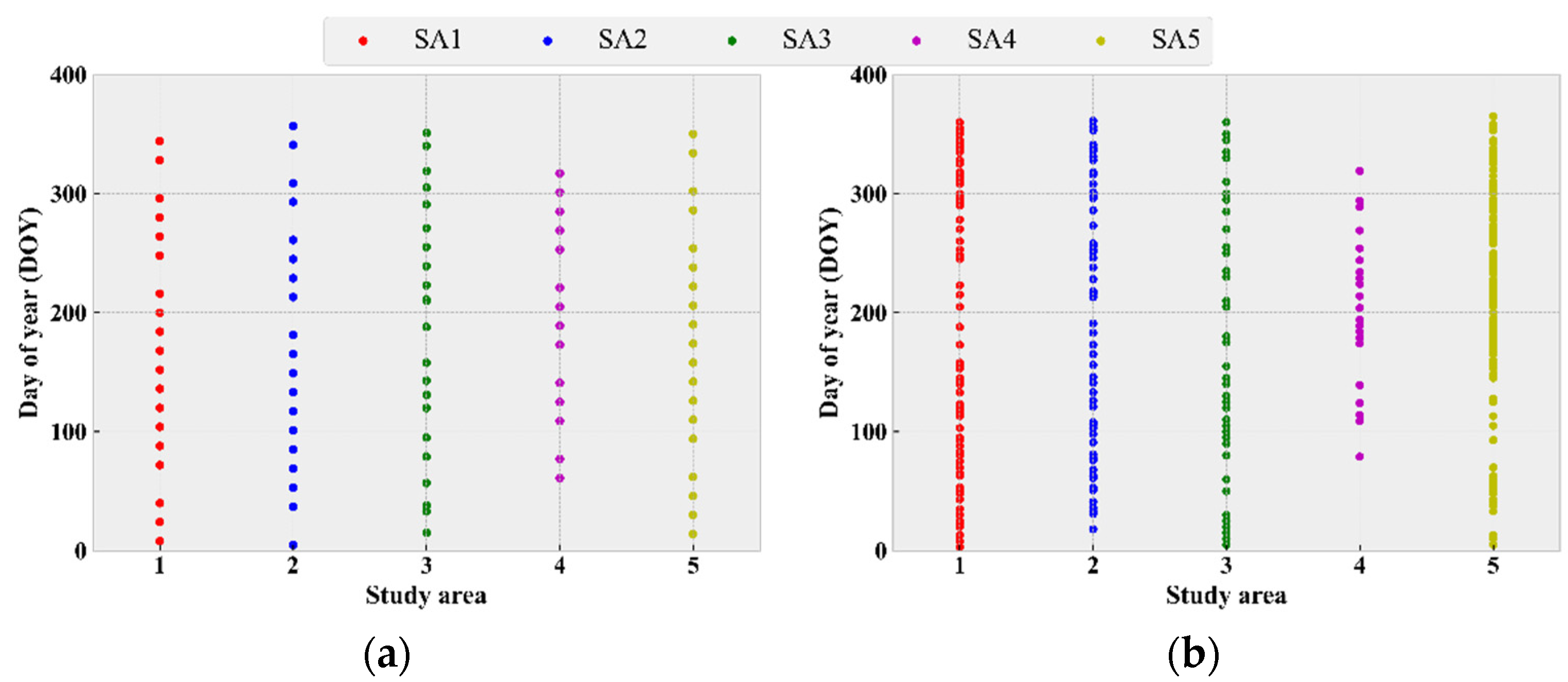
2.2.2. Multi-Temporal-Resolution Images
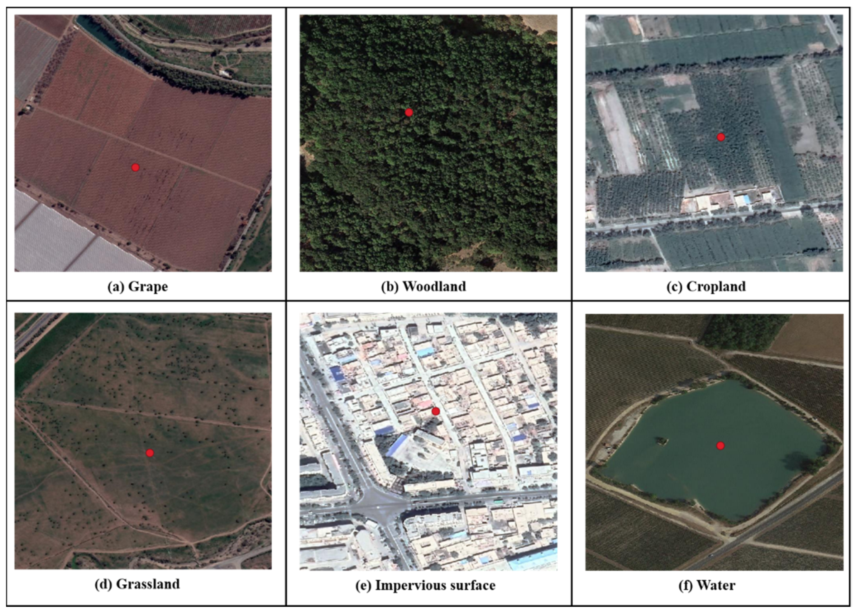
2.2.3. Sample Collection
3. Methods
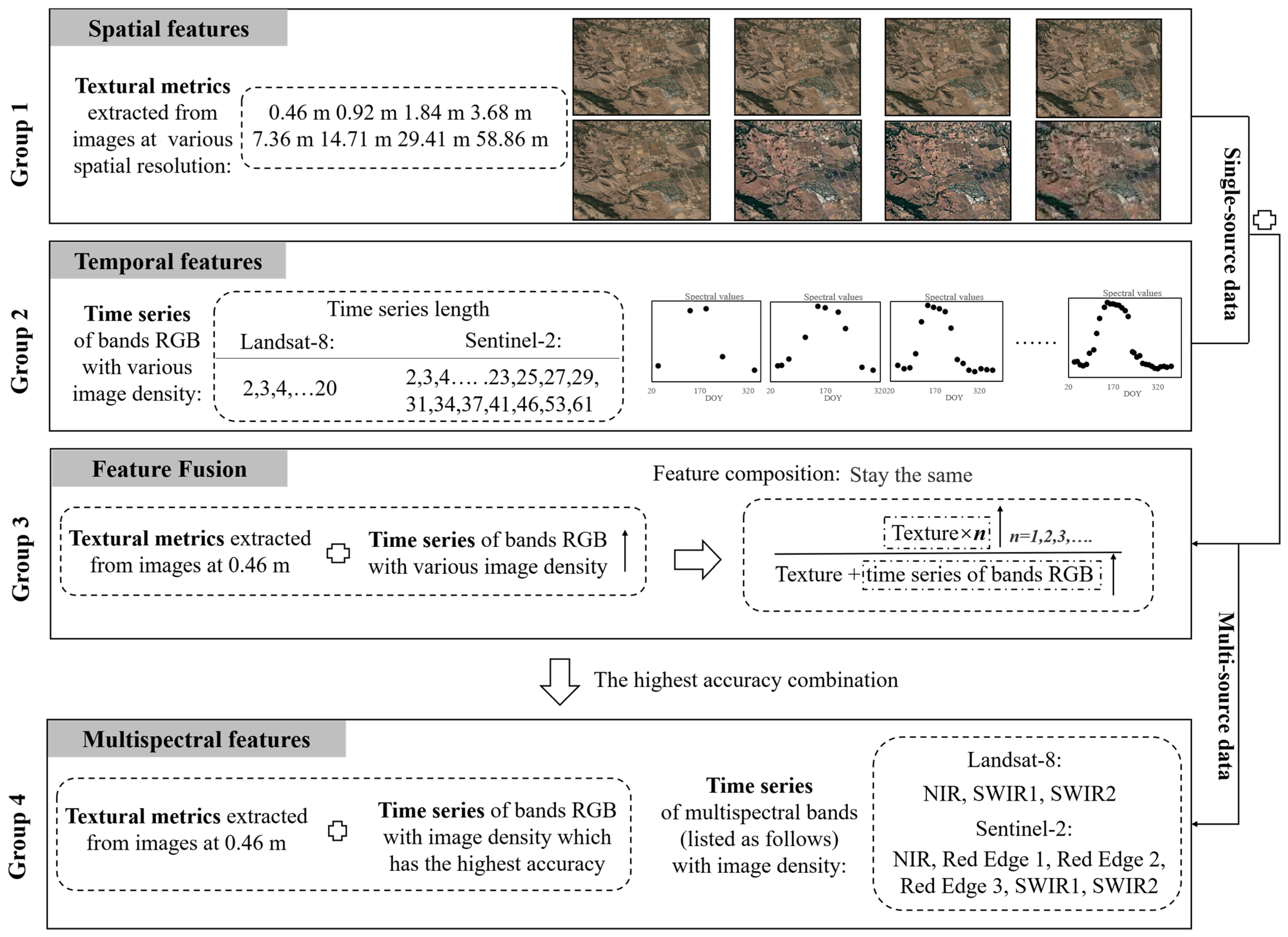
3.1. Spatial Features
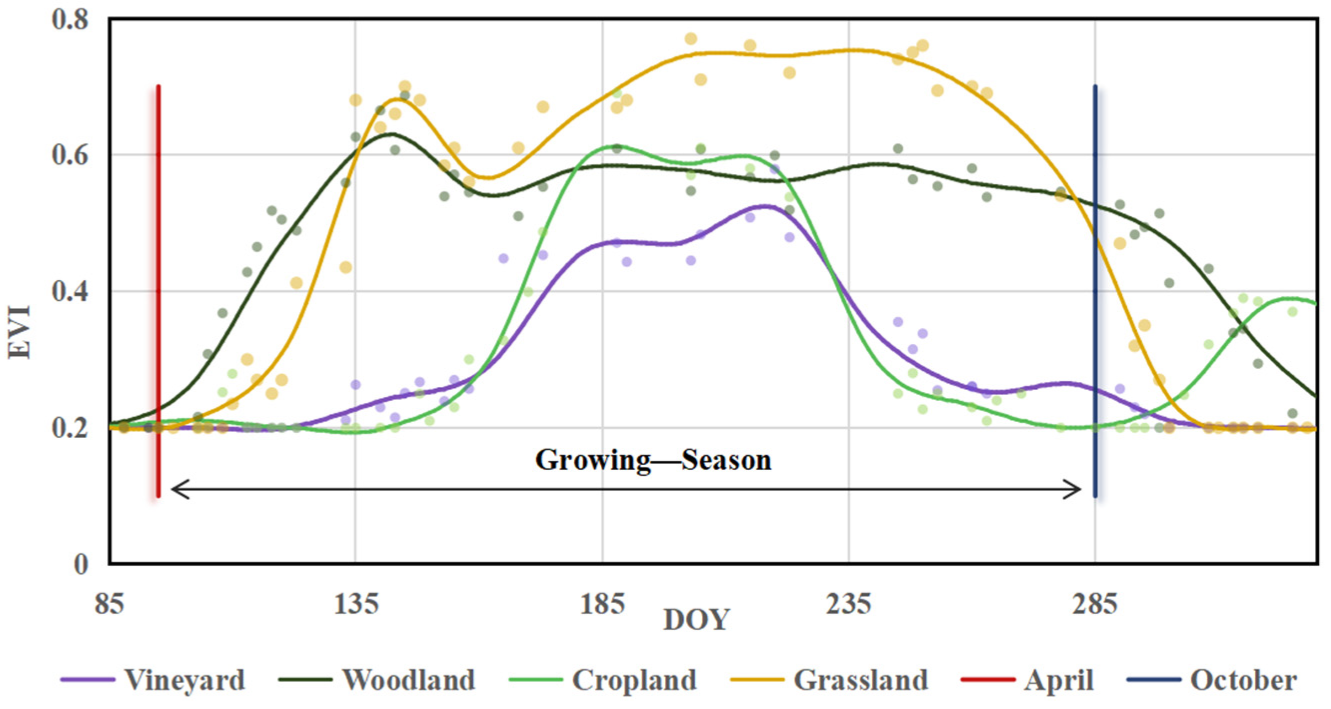
3.2. Temporal Features
3.3. Classification
3.4. Random Forest Classifier
3.5. Accuracy Assessment and Comparison
4. Results
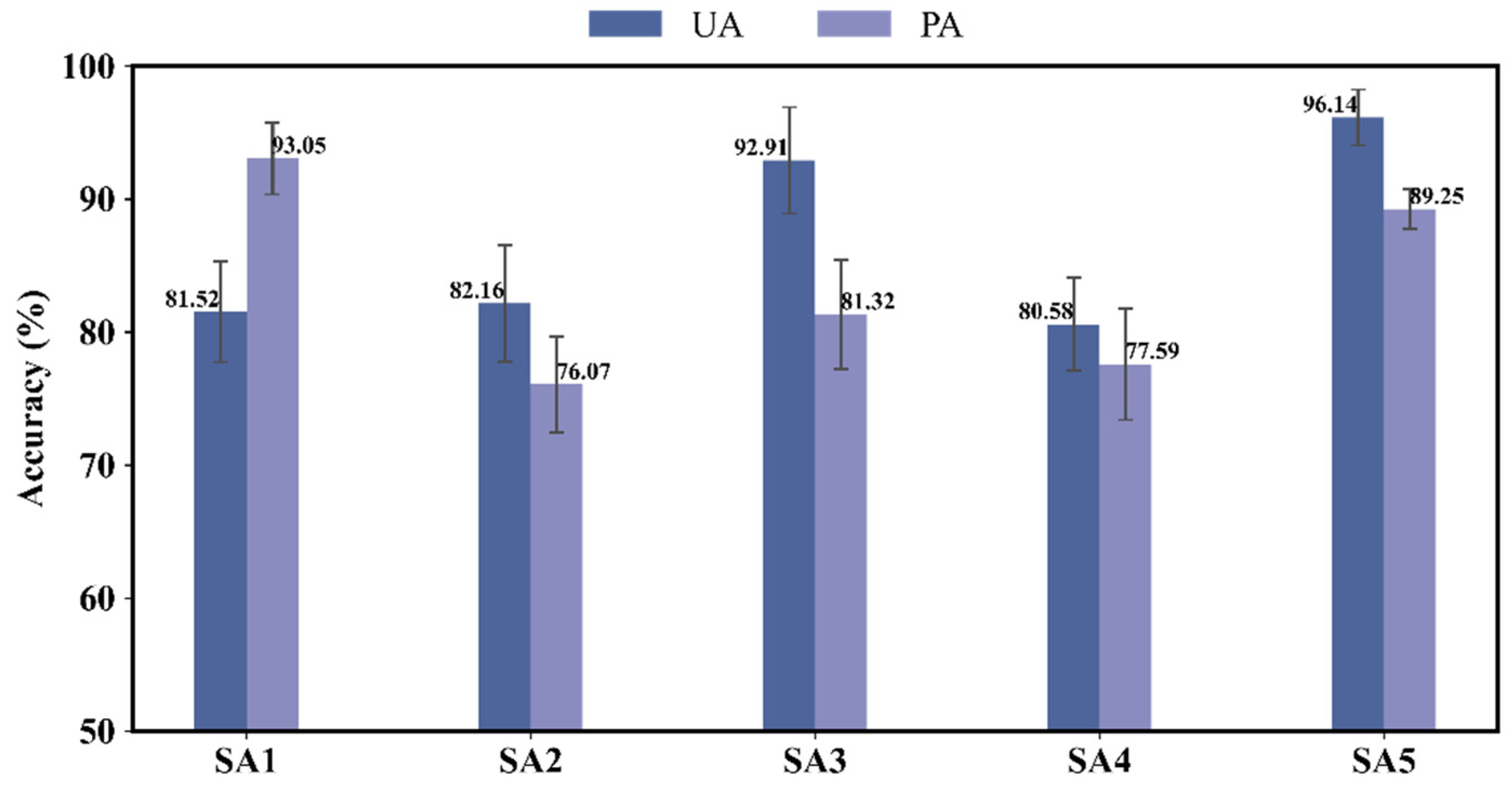
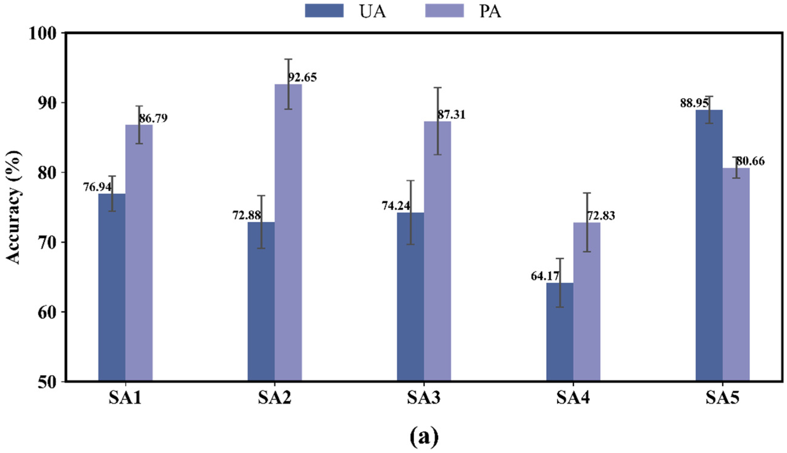
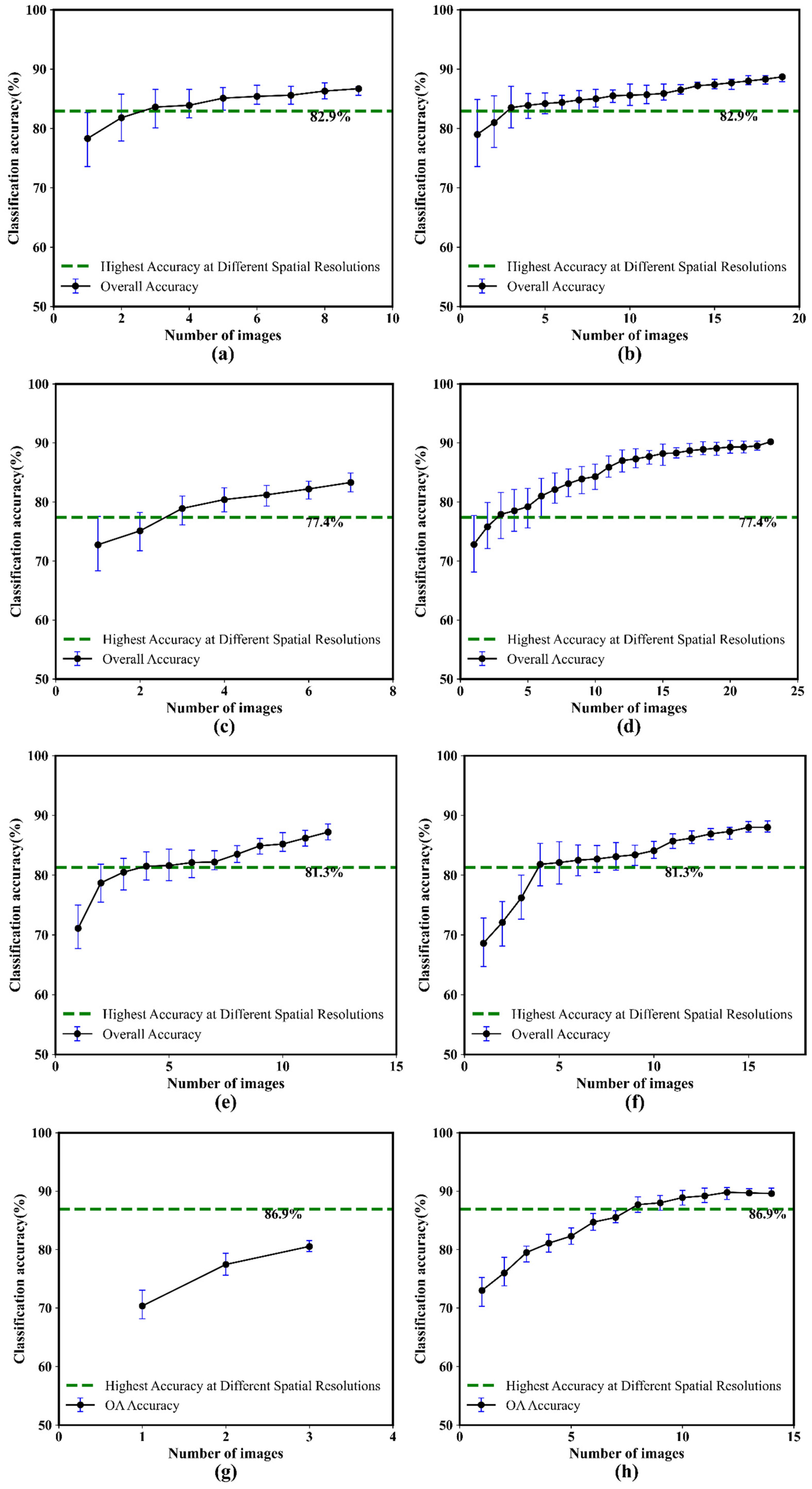
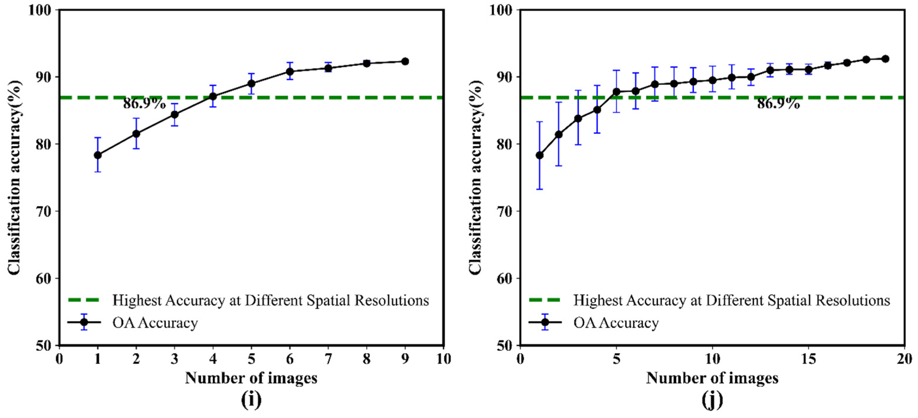
4.1. Classification Accuracies of Images at Various Spatial Resolutions
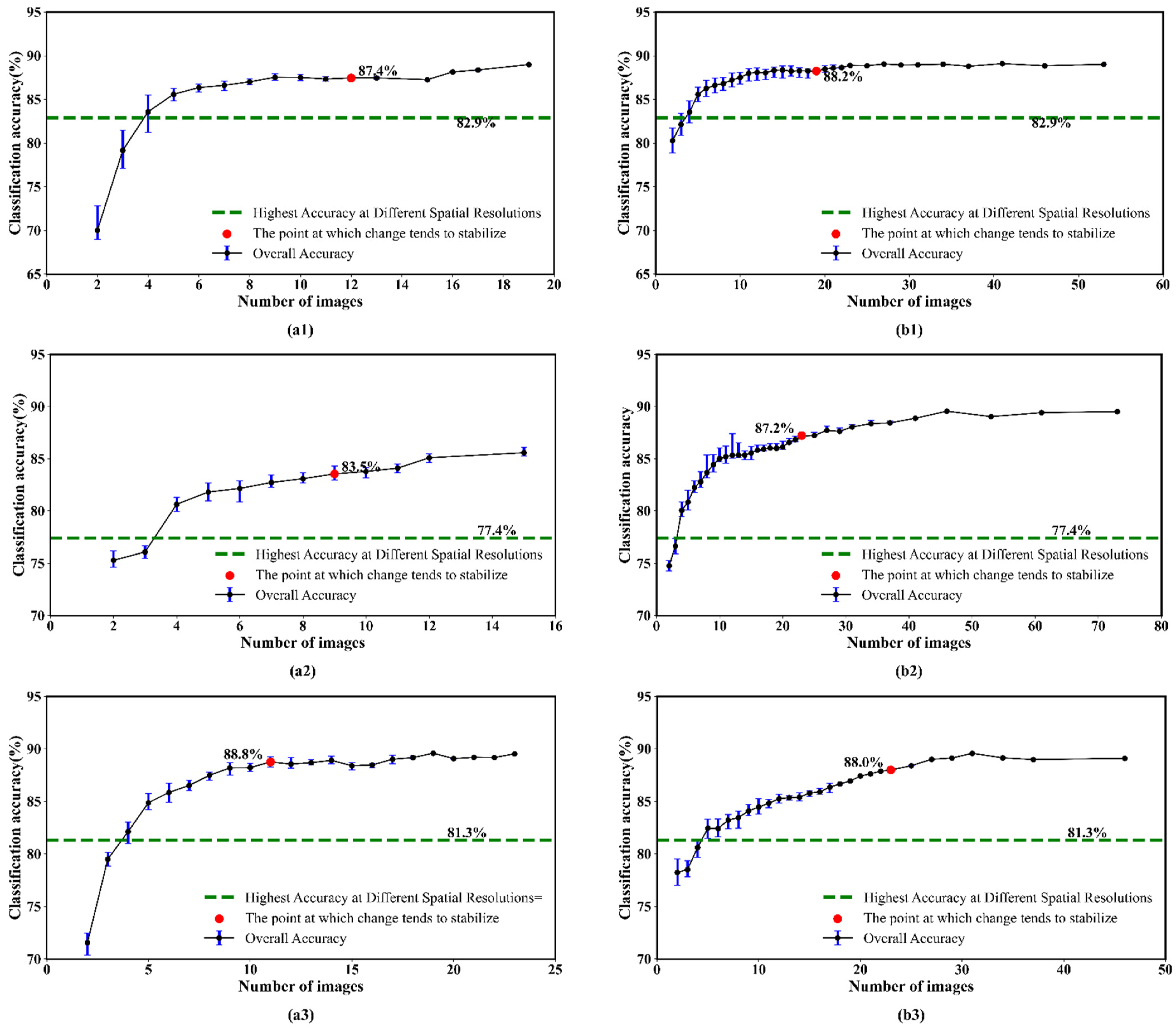
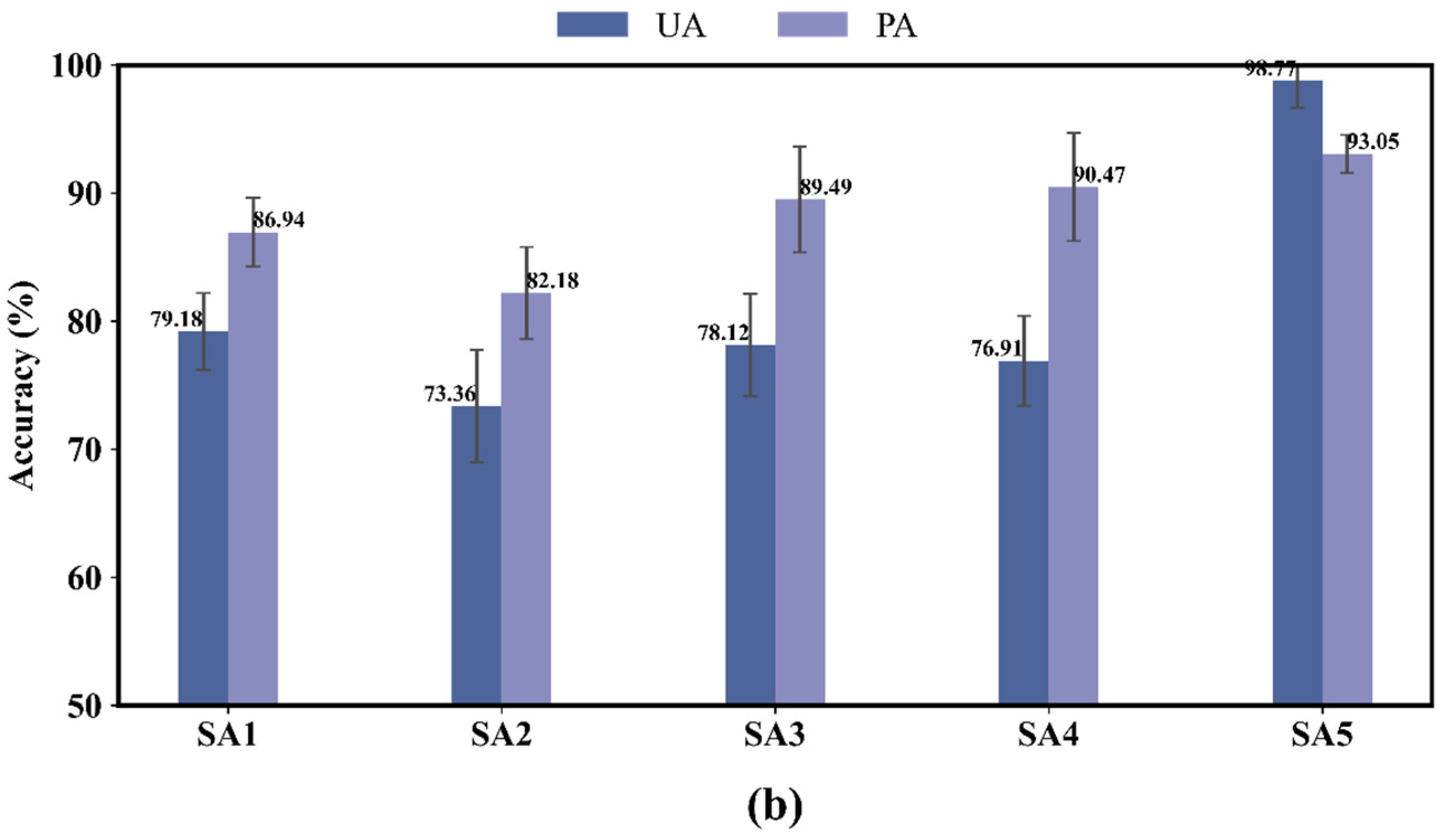
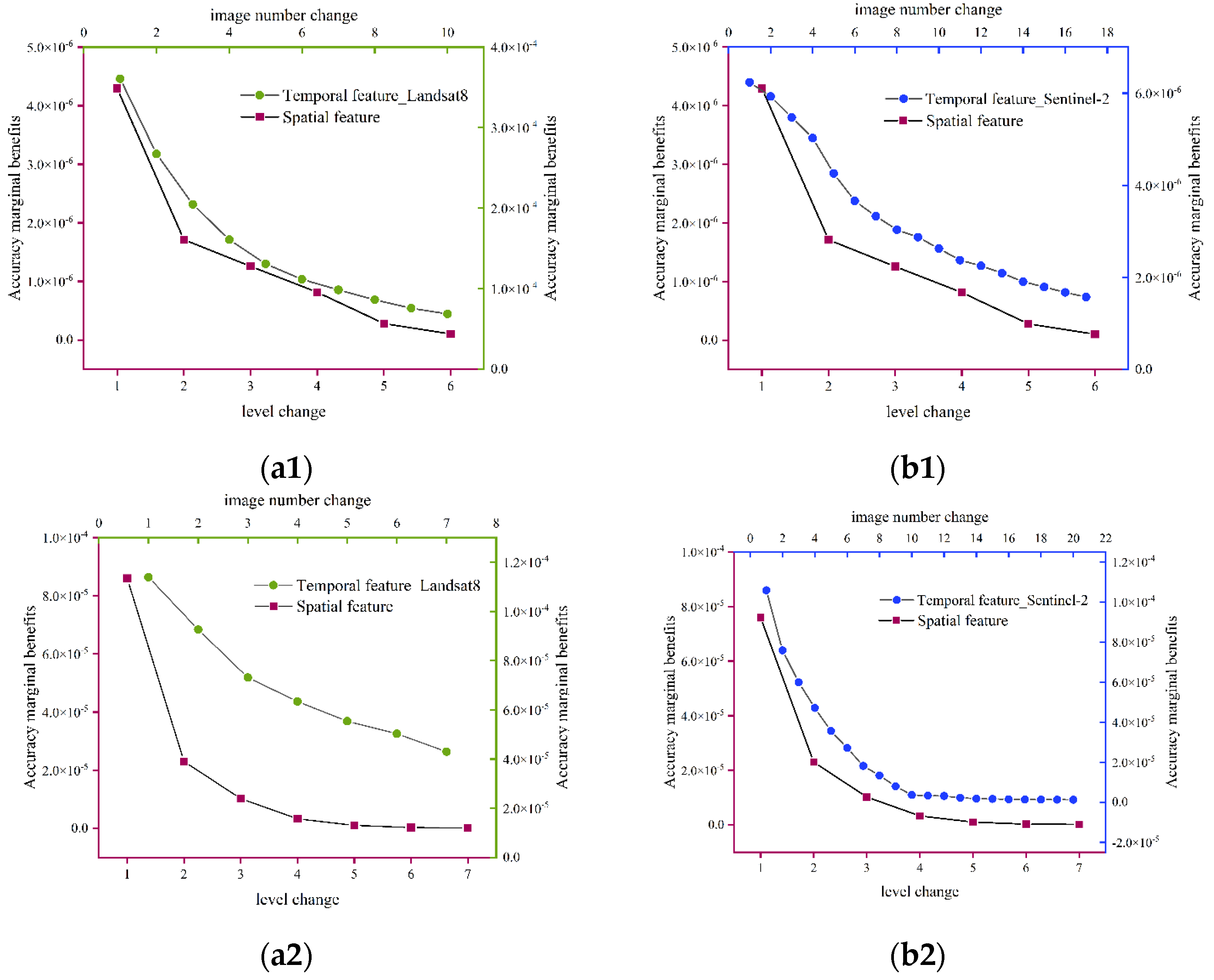
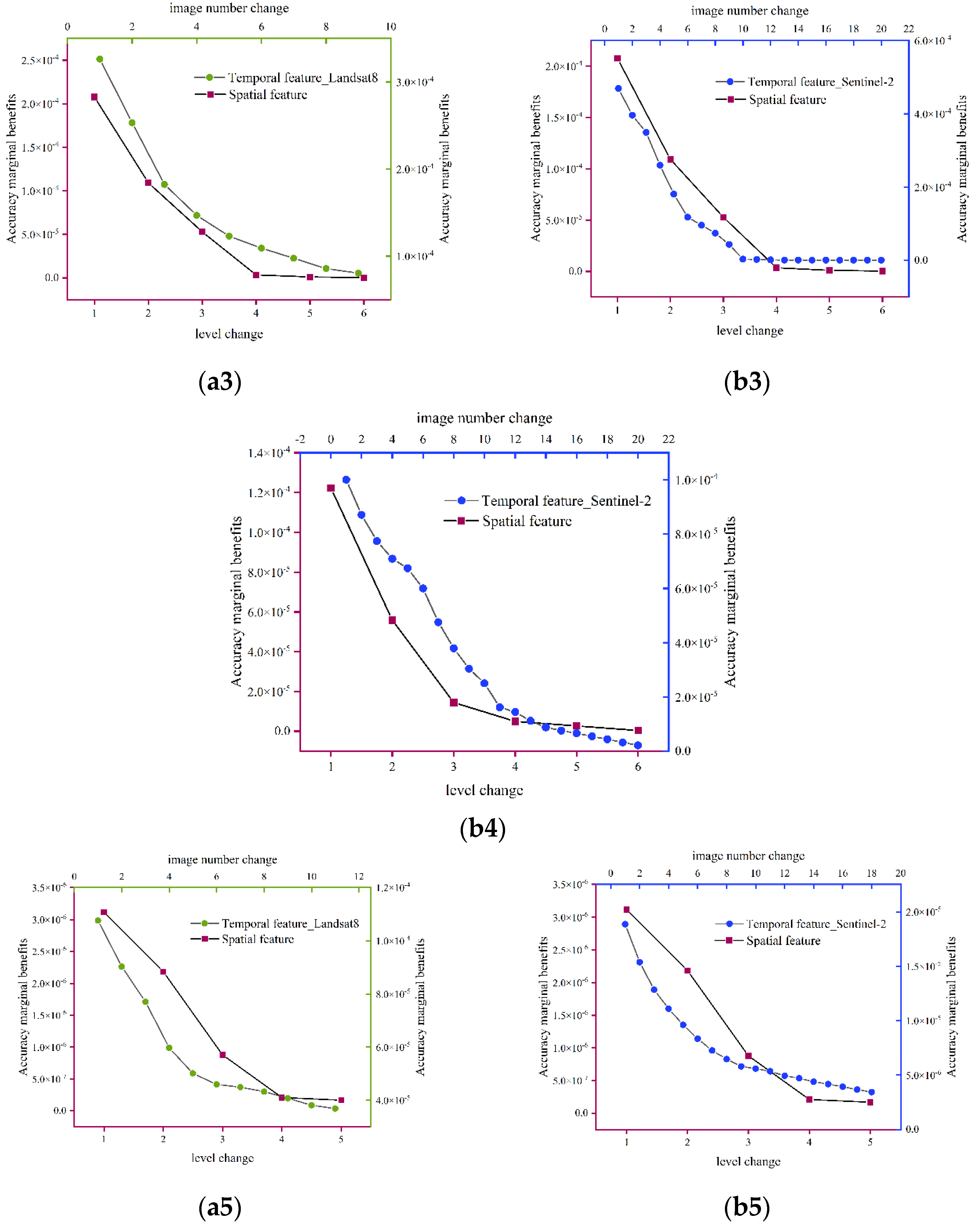
4.2. Classification Accuracies of Images at Various Temporal Resolutions
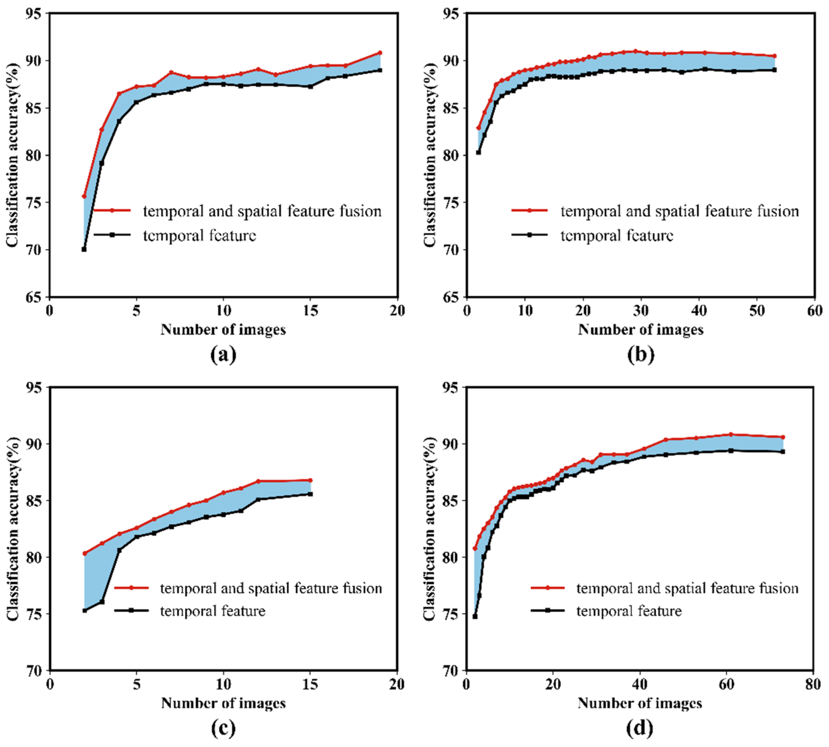
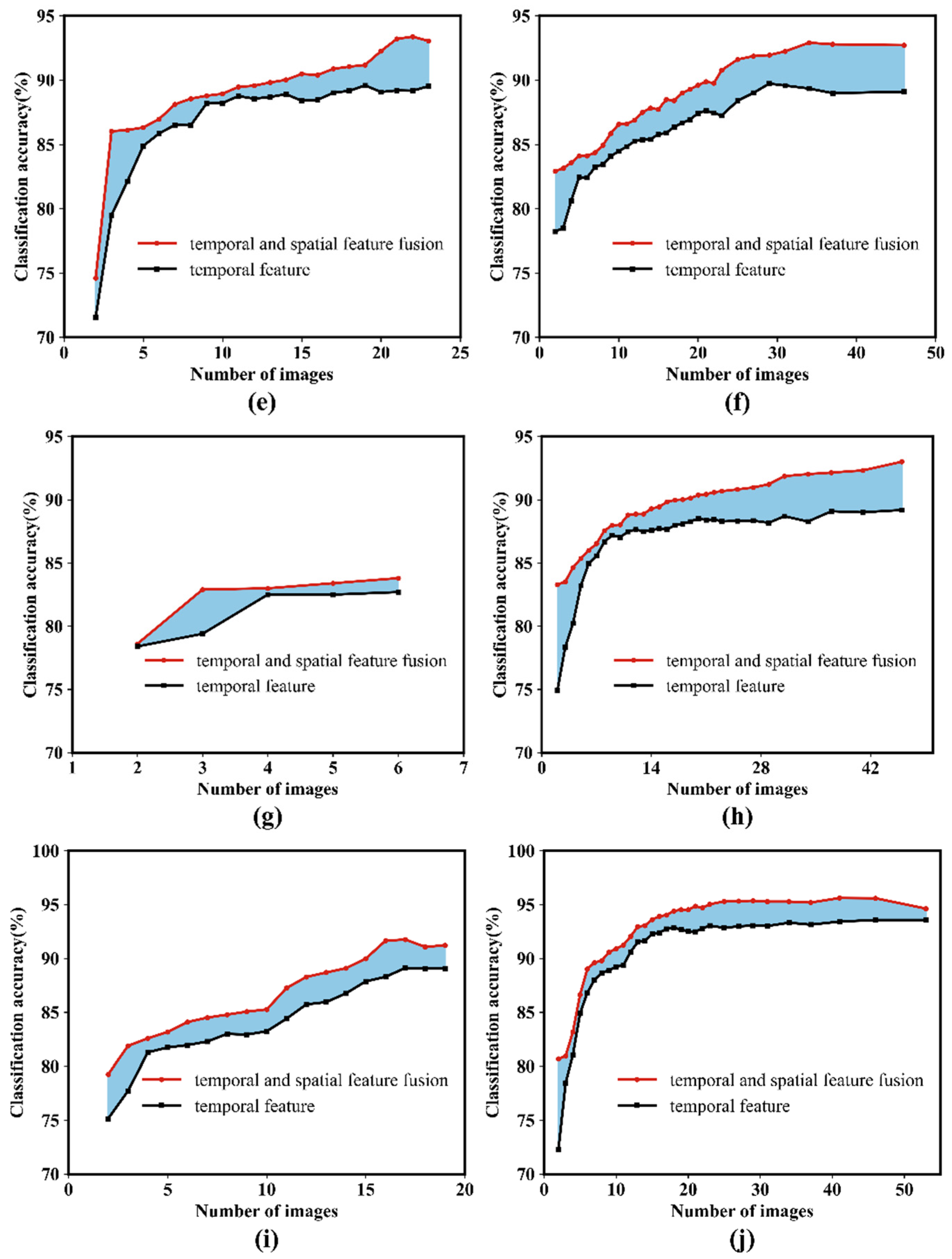
4.3. Mapping Performance Comparison of Single-Source Data
4.4. Mapping Performance Comparison of Multi-Source Data
4.5. Mapping Results
5. Discussion
6. Conclusions
Author Contributions
Funding
Institutional Review Board Statement
Informed Consent Statement
Data Availability Statement
Conflicts of Interest
References
- Kozhoridze, G.; Orlovsky, N.; Orlovsky, L.; Blumberg, D.G.; Golan-Goldhirsh, A. Classification-based mapping of trees in commercial orchards and natural forests. Int. J. Remote Sens. 2018, 39, 8784–8797. [Google Scholar] [CrossRef]
- Cen, Y.; Li, L.; Guo, L.; Li, C.; Jiang, G. Organic management enhances both ecological and economic profitability of apple orchard: A case study in Shandong Peninsula. Sci. Hortic. 2020, 265, 109201. [Google Scholar] [CrossRef]
- Chen, Z.; Sarkar, A.; Hasan, A.K.; Li, X.; Xia, X. Evaluation of farmers’ ecological cognition in responses to specialty orchard fruit planting behavior: Evidence in Shaanxi and Ningxia, China. Agriculture 2021, 11, 1056. [Google Scholar] [CrossRef]
- Yang, Y.; Huang, Q.; Wu, W.; Luo, J.; Gao, L.; Dong, W.; Wu, T.; Hu, X. Geo-parcel based crop identification by integrating high spatial-temporal resolution imagery from multi-source satellite data. Remote Sens. 2017, 9, 1298. [Google Scholar] [CrossRef] [Green Version]
- Ashourloo, D.; Shahrabi, H.S.; Azadbakht, M.; Aghighi, H.; Nematollahi, H.; Alimohammadi, A.; Matkan, A.A. Automatic canola mapping using time series of sentinel 2 images. ISPRS J. Photogramm. Remote Sens. 2019, 156, 63–76. [Google Scholar] [CrossRef]
- Johansen, K.; Phinn, S.; Witte, C.; Philip, S.; Newton, L. Mapping banana plantations from object-oriented classification of SPOT-5 imagery. Photogramm. Eng. Remote Sens. 2009, 75, 1069–1081. [Google Scholar] [CrossRef] [Green Version]
- Xu, H.; Qi, S.; Gong, P.; Liu, C.; Wang, J. Long-term monitoring of citrus orchard dynamics using time-series Landsat data: A case study in southern China. Int. J. Remote Sens. 2018, 39, 8271–8292. [Google Scholar] [CrossRef]
- Chen, B.; Huang, B.; Xu, B. Multi-source remotely sensed data fusion for improving land cover classification. ISPRS J. Photogramm. Remote Sens. 2017, 124, 27–39. [Google Scholar] [CrossRef]
- Duarte, L.; Silva, P.; Teodoro, A.C. Development of a QGIS plugin to obtain parameters and elements of plantation trees and vineyards with aerial photographs. ISPRS Int. J. Geo.-Inf. 2018, 7, 109. [Google Scholar] [CrossRef] [Green Version]
- Maschler, J.; Atzberger, C.; Immitzer, M. Individual tree crown segmentation and classification of 13 tree species using airborne hyperspectral data. Remote Sens. 2018, 10, 1218. [Google Scholar] [CrossRef]
- Duarte, L.; Teodoro, A.C.; Monteiro, A.T.; Cunha, M.; Gonçalves, H. QPhenoMetrics: An open source software application to assess vegetation phenology metrics. Comput. Electron. Agric. 2018, 148, 82–94. [Google Scholar] [CrossRef]
- Dalponte, M.; Marzini, S.; Solano-Correa, Y.T.; Tonon, G.; Vescovo, L.; Gianelle, D. Mapping forest windthrows using high spatial resolution multispectral satellite images. Int. J. Appl. Earth Obs. Geoinf. 2020, 93, 102206. [Google Scholar] [CrossRef]
- Solano-Correa, Y.T.; Bovolo, F.; Bruzzone, L. Generation of homogeneous VHR time series by nonparametric regression of multisensor bitemporal images. IEEE Trans. Geosci. Remote Sens. 2019, 57, 7579–7593. [Google Scholar] [CrossRef]
- Solano-Correa, Y.T.; Bovolo, F.; Bruzzone, L. An approach for unsupervised change detection in multitemporal VHR images acquired by different multispectral sensors. Remote Sens. 2018, 10, 533. [Google Scholar] [CrossRef] [Green Version]
- Pehani, P.; Čotar, K.; Marsetič, A.; Zaletelj, J.; Oštir, K. Automatic geometric processing for very high resolution optical satellite data based on vector roads and orthophotos. Remote Sens. 2016, 8, 343. [Google Scholar] [CrossRef] [Green Version]
- Vahidi, H.; Klinkenberg, B.; Johnson, B.A.; Moskal, L.M.; Yan, W. Mapping the individual trees in urban orchards by incorporating Volunteered Geographic Information and very high resolution optical remotely sensed data: A template matching-based approach. Remote Sens. 2018, 10, 1134. [Google Scholar] [CrossRef] [Green Version]
- Higginbottom, T.P.; Symeonakis, E.; Meyer, H.; van der Linden, S. Mapping fractional woody cover in semi-arid savannahs using multi-seasonal composites from Landsat data. ISPRS J. Photogramm. Remote Sens. 2018, 139, 88–102. [Google Scholar] [CrossRef] [Green Version]
- Peña, M.; Liao, R.; Brenning, A. Using spectrotemporal indices to improve the fruit-tree crop classification accuracy. ISPRS J. Photogramm. Remote Sens. 2017, 128, 158–169. [Google Scholar] [CrossRef]
- Sarron, J.; Malézieux, É.; Sané, C.A.B.; Faye, É. Mango yield mapping at the orchard scale based on tree structure and land cover assessed by UAV. Remote Sens. 2018, 10, 1900. [Google Scholar] [CrossRef] [Green Version]
- Brinkhoff, J.; Vardanega, J.; Robson, A.J. Land cover classification of nine perennial crops using sentinel-1 and-2 data. Remote Sens. 2019, 12, 96. [Google Scholar] [CrossRef]
- Fisher, J.R.; Acosta, E.A.; Dennedy-Frank, P.J.; Kroeger, T.; Boucher, T.M. Impact of satellite imagery spatial resolution on land use classification accuracy and modeled water quality. Remote Sens. Ecol. Conserv. 2018, 4, 137–149. [Google Scholar] [CrossRef]
- Räsänen, A.; Virtanen, T. Data and resolution requirements in mapping vegetation in spatially heterogeneous landscapes. Remote Sens. Environ. 2019, 230, 111207. [Google Scholar] [CrossRef]
- Hao, P.; Zhan, Y.; Wang, L.; Niu, Z.; Shakir, M. Feature selection of time series MODIS data for early crop classification using random forest: A case study in Kansas, USA. Remote Sens. 2015, 7, 5347–5369. [Google Scholar] [CrossRef] [Green Version]
- Xu, Y.; Yu, L.; Peng, D.; Cai, X.; Cheng, Y.; Zhao, J.; Zhao, Y.; Feng, D.; Hackman, K.; Huang, X. Exploring the temporal density of Landsat observations for cropland mapping: Experiments from Egypt, Ethiopia, and South Africa. Int. J. Remote Sens. 2018, 39, 7328–7349. [Google Scholar] [CrossRef]
- Mirás-Avalos, J.M.; Araujo, E.S. Optimization of vineyard water management: Challenges, strategies, and perspectives. Water 2021, 13, 746. [Google Scholar] [CrossRef]
- Carrasco-Benavides, M.; Ortega-Farías, S.; Gil, P.M.; Knopp, D.; Morales-Salinas, L.; Lagos, L.O.; de la Fuente, D.; López-Olivari, R.; Fuentes, S. Assessment of the vineyard water footprint by using ancillary data and EEFlux satellite images. Examples in the Chilean central zone. Sci. Total Environ. 2022, 811, 152452. [Google Scholar] [CrossRef]
- Fraga, H.; Pinto, J.G.; Santos, J.A. Climate change projections for chilling and heat forcing conditions in European vineyards and olive orchards: A multi-model assessment. Clim. Chang. 2019, 152, 179–193. [Google Scholar] [CrossRef]
- Beck, H.E.; Zimmermann, N.E.; McVicar, T.R.; Vergopolan, N.; Berg, A.; Wood, E.F. Present and future Köppen-Geiger climate classification maps at 1-km resolution. Sci. Data 2018, 5, 1–12. [Google Scholar] [CrossRef] [Green Version]
- Medellín-Azuara, J.; Escriva-Bou, A.; Abatzoglou, J.A.; Viers, J.H.; Cole, S.A.; Rodríguez-Flores, J.M.; Sumner, D.A. Economic Impacts of the 2021 Drought on California Agriculture; University of California: Merced, CA, USA, 2022. [Google Scholar]
- Chuang, Y.-C.M.; Shiu, Y.-S. A comparative analysis of machine learning with WorldView-2 pan-sharpened imagery for tea crop mapping. Sensors 2016, 16, 594. [Google Scholar] [CrossRef] [Green Version]
- Madonsela, S.; Cho, M.A.; Mathieu, R.; Mutanga, O.; Ramoelo, A.; Kaszta, Ż.; Van De Kerchove, R.; Wolff, E. Multi-phenology WorldView-2 imagery improves remote sensing of savannah tree species. Int. J. Appl. Earth Obs. Geoinf. 2017, 58, 65–73. [Google Scholar] [CrossRef]
- Li, J.; Chen, B. Global revisit interval analysis of Landsat-8-9 and Sentinel-2A-2B data for terrestrial monitoring. Sensors 2020, 20, 6631. [Google Scholar] [CrossRef]
- Mahdianpari, M.; Salehi, B.; Mohammadimanesh, F.; Homayouni, S.; Gill, E. The first wetland inventory map of newfoundland at a spatial resolution of 10 m using sentinel-1 and sentinel-2 data on the google earth engine cloud computing platform. Remote Sens. 2018, 11, 43. [Google Scholar] [CrossRef] [Green Version]
- Tarko, A.; Tsendbazar, N.-E.; De Bruin, S.; Bregt, A.K. Producing consistent visually interpreted land cover reference data: Learning from feedback. Int. J. Digital Earth 2021, 14, 52–70. [Google Scholar] [CrossRef]
- Fan, L.; Yang, J.; Sun, X.; Zhao, F.; Liang, S.; Duan, D.; Chen, H.; Xia, L.; Sun, J.; Yang, P. The effects of Landsat image acquisition date on winter wheat classification in the North China Plain. ISPRS J. Photogramm. Remote Sens. 2022, 187, 1–13. [Google Scholar] [CrossRef]
- More, A.; Rana, D.P. Review of random forest classification techniques to resolve data imbalance. In Proceedings of the 2017 1st International Conference on Intelligent Systems and Information Management (ICISIM), Aurangabad, India, 5–6 October 2017; pp. 72–78. [Google Scholar]
- Tassi, A.; Gigante, D.; Modica, G.; Di Martino, L.; Vizzari, M. Pixel-vs. Object-based landsat 8 data classification in google earth engine using random forest: The case study of maiella national park. Remote Sens. 2021, 13, 2299. [Google Scholar] [CrossRef]
- Tassi, A.; Vizzari, M. Object-oriented lulc classification in google earth engine combining snic, glcm, and machine learning algorithms. Remote Sens. 2020, 12, 3776. [Google Scholar] [CrossRef]
- Haralick, R.M.; Shanmugam, K.; Dinstein, I.H. Textural features for image classification. IEEE Trans. Syst. Man Cybern. 1973, 3, 610–621. [Google Scholar] [CrossRef] [Green Version]
- Haralick, R.M. Statistical and structural approaches to texture. Proc. IEEE 1979, 67, 786–804. [Google Scholar] [CrossRef]
- Phan, T.N.; Kuch, V.; Lehnert, L.W. Land Cover Classification using Google Earth Engine and Random Forest Classifier—The Role of Image Composition. Remote Sens. 2020, 12, 2411. [Google Scholar] [CrossRef]
- White, M.A.; Thornton, P.E.; Running, S.W. A continental phenology model for monitoring vegetation responses to interannual climatic variability. Global Biogeochem. Cycles 1997, 11, 217–234. [Google Scholar] [CrossRef]
- Liu, H.Q.; Huete, A. A feedback based modification of the NDVI to minimize canopy background and atmospheric noise. IEEE Trans. Geosci. Remote Sens. 1995, 33, 457–465. [Google Scholar] [CrossRef]
- Breiman, L. Random forests. Mach. Learn. 2001, 45, 5–32. [Google Scholar] [CrossRef] [Green Version]
- Amani, M.; Mahdavi, S.; Afshar, M.; Brisco, B.; Huang, W.; Mohammad Javad Mirzadeh, S.; White, L.; Banks, S.; Montgomery, J.; Hopkinson, C. Canadian wetland inventory using Google Earth Engine: The first map and preliminary results. Remote Sens. 2019, 11, 842. [Google Scholar] [CrossRef] [Green Version]
- Huang, C.; Zhang, C.; He, Y.; Liu, Q.; Li, H.; Su, F.; Liu, G.; Bridhikitti, A. Land Cover Mapping in Cloud-Prone Tropical Areas Using Sentinel-2 Data: Integrating Spectral Features with Ndvi Temporal Dynamics. Remote Sens. 2020, 12, 1163. [Google Scholar] [CrossRef] [Green Version]
- Teluguntla, P.; Thenkabail, P.S.; Oliphant, A.; Xiong, J.; Gumma, M.K.; Congalton, R.G.; Yadav, K.; Huete, A. A 30-m landsat-derived cropland extent product of Australia and China using random forest machine learning algorithm on Google Earth Engine cloud computing platform. ISPRS J. Photogramm. Remote Sens. 2018, 144, 325–340. [Google Scholar] [CrossRef]
- Zhang, T.; Su, J.; Xu, Z.; Luo, Y.; Li, J. Sentinel-2 satellite imagery for urban land cover classification by optimized random forest classifier. Appl. Sci. 2021, 11, 543. [Google Scholar] [CrossRef]
- Mahdianpari, M.; Salehi, B.; Mohammadimanesh, F.; Motagh, M. Random forest wetland classification using ALOS-2 L-band, RADARSAT-2 C-band, and TerraSAR-X imagery. ISPRS J. Photogramm. Remote Sens. 2017, 130, 13–31. [Google Scholar] [CrossRef]
- Xia, J.; Falco, N.; Benediktsson, J.A.; Du, P.; Chanussot, J. Hyperspectral image classification with rotation random forest via KPCA. IEEE J. Sel. Top. Appl. Earth Obs. Remote Sens. 2017, 10, 1601–1609. [Google Scholar] [CrossRef] [Green Version]
- Abdel-Rahman, E.M.; Mutanga, O.; Adam, E.; Ismail, R. Detecting Sirex noctilio grey-attacked and lightning-struck pine trees using airborne hyperspectral data, random forest and support vector machines classifiers. ISPRS J. Photogramm. Remote Sens. 2014, 88, 48–59. [Google Scholar] [CrossRef]
- Rodriguez-Galiano, V.F.; Chica-Rivas, M. Evaluation of different machine learning methods for land cover mapping of a Mediterranean area using multi-seasonal Landsat images and Digital Terrain Models. Int. J. Digital Earth 2014, 7, 492–509. [Google Scholar] [CrossRef]
- Nitze, I.; Schulthess, U.; Asche, H. Comparison of machine learning algorithms random forest, artificial neural network and support vector machine to maximum likelihood for supervised crop type classification. In Proceedings of the 4th GEOBIA, Rio de Janeiro, Brazil, 7–9 May 2012; Volume 79, p. 3540. [Google Scholar]
- Song, A.; Choi, J. Fully convolutional networks with multiscale 3D filters and transfer learning for change detection in high spatial resolution satellite images. Remote Sens. 2020, 12, 799. [Google Scholar] [CrossRef] [Green Version]
- Maxwell, A.E.; Warner, T.A.; Fang, F. Implementation of machine-learning classification in remote sensing: An applied review. Int. J. Remote Sens. 2018, 39, 2784–2817. [Google Scholar] [CrossRef] [Green Version]
- Tamiminia, H.; Salehi, B.; Mahdianpari, M.; Quackenbush, L.; Adeli, S.; Brisco, B. Google Earth Engine for geo-big data applications: A meta-analysis and systematic review. ISPRS J. Photogramm. Remote Sens. 2020, 164, 152–170. [Google Scholar] [CrossRef]
- Sadras, V.; Bongiovanni, R. Use of Lorenz curves and Gini coefficients to assess yield inequality within paddocks. Field Crops Res. 2004, 90, 303–310. [Google Scholar] [CrossRef]
- Cánovas-García, F.; Alonso-Sarría, F.; Gomariz-Castillo, F.; Oñate-Valdivieso, F. Modification of the random forest algorithm to avoid statistical dependence problems when classifying remote sensing imagery. Comput. Geosci. 2017, 103, 1–11. [Google Scholar] [CrossRef] [Green Version]
- Ghimire, B.; Rogan, J.; Galiano, V.R.; Panday, P.; Neeti, N. An evaluation of bagging, boosting, and random forests for land-cover classification in Cape Cod, Massachusetts, USA. GISci. Remote Sens. 2012, 49, 623–643. [Google Scholar] [CrossRef]
- Yan, X.; Li, J.; Yang, D.; Li, J.; Ma, T.; Su, Y.; Shao, J.; Zhang, R. A Random Forest Algorithm for Landsat Image Chromatic Aberration Restoration Based on GEE Cloud Platform—A Case Study of Yucatán Peninsula, Mexico. Remote Sens. 2022, 14, 5154. [Google Scholar] [CrossRef]
- Congalton, R.G. A review of assessing the accuracy of classifications of remotely sensed data. Remote Sens. Environ. 1991, 37, 35–46. [Google Scholar] [CrossRef]
- Story, M.; Congalton, R.G. Accuracy assessment: A user’s perspective. Photogramm. Eng. Remote Sens. 1986, 52, 397–399. [Google Scholar]
- Yuh, Y.G.; Tracz, W.; Matthews, H.D.; Turner, S.E. Application of machine learning approaches for land cover monitoring in northern Cameroon. Ecol. Inf. 2022, 74, 101955. [Google Scholar] [CrossRef]
- Liu, L.; Zhang, X.; Gao, Y.; Chen, X.; Shuai, X.; Mi, J. Finer-resolution mapping of global land cover: Recent developments, consistency analysis, and prospects. J. Remote 2021, 2021, 5289697. [Google Scholar] [CrossRef]
- Sari, I.L.; Weston, C.J.; Newnham, G.J.; Volkova, L. Assessing accuracy of land cover change maps derived from automated digital processing and visual interpretation in tropical forests in Indonesia. Remote Sens. 2021, 13, 1446. [Google Scholar] [CrossRef]
- Yang, Y.; Yang, D.; Wang, X.; Zhang, Z.; Nawaz, Z. Testing accuracy of land cover classification algorithms in the qilian mountains based on gee cloud platform. Remote Sens. 2021, 13, 5064. [Google Scholar] [CrossRef]
- Zhang, L.; Liu, Z.; Liu, D.; Xiong, Q.; Yang, N.; Ren, T.; Zhang, C.; Zhang, X.; Li, S. Crop mapping based on historical samples and new training samples generation in Heilongjiang Province, China. Sustainability 2019, 11, 5052. [Google Scholar] [CrossRef] [Green Version]
- Wang, L.; Liu, J.; Gao, J.; Yang, L.; Yang, F.; Wang, X. Relationship between accuracy of winter wheat area remote sensing identification and spatial resolution. Trans. Chin. Soc. Agric. Eng. 2016, 32, 152–160. [Google Scholar] [CrossRef]
- Cao, J.; Leng, W.; Liu, K.; Liu, L.; He, Z.; Zhu, Y. Object-based mangrove species classification using unmanned aerial vehicle hyperspectral images and digital surface models. Remote Sens. 2018, 10, 89. [Google Scholar] [CrossRef] [Green Version]
- Dong, J.; Xiao, X.; Kou, W.; Qin, Y.; Zhang, G.; Li, L.; Jin, C.; Zhou, Y.; Wang, J.; Biradar, C. Tracking the dynamics of paddy rice planting area in 1986–2010 through time series Landsat images and phenology-based algorithms. Remote Sens. Environ. 2015, 160, 99–113. [Google Scholar] [CrossRef]
- Wang, L.; Wang, J.; Zhang, X.; Wang, L.; Qin, F. Deep segmentation and classification of complex crops using multi-feature satellite imagery. Comput. Electron. Agric. 2022, 200, 107249. [Google Scholar] [CrossRef]
- Anastasiou, E.; Balafoutis, A.; Darra, N.; Psiroukis, V.; Biniari, A.; Xanthopoulos, G.; Fountas, S. Satellite and proximal sensing to estimate the yield and quality of table grapes. Agriculture 2018, 8, 94. [Google Scholar] [CrossRef]
- Tuck, B.; Gartner, W.; Appiah, G. Vineyards and Grapes of the North; University of Minnesota: Minneapolis, MI, USA, 2016. [Google Scholar]


| Study Area | Climate Type | Max_Temp | Min_Temp | Aver_Prec |
|---|---|---|---|---|
| SA1 | Temperate sub-humid continental monsoon | 17 °C | 7 °C | 556 mm |
| SA2 | Warm temperate monsoon | 28.8 °C | −2.3 °C | 664 mm |
| SA3 | Continental desert | 49.6 °C | −28.7 °C | 118 mm |
| SA4 | Temperate marine | 17 °C | 10 °C | 656 mm |
| SA5 | Mediterranean | 5 °C | 13.4 °C | 510 mm |
| Study Area | VHR Images | Landsat-8 and Sentinel-2 | ||
|---|---|---|---|---|
| Acquisition Date | Selected Bands | Acquisition Date | Selected Bands | |
| SA1 | 14 August 2020 | Blue Green Red | 2020–2021 | Blue, green, red NIR, SWIR1, SWIR2 Red edge 1, red edge 2 red edge 3 |
| SA2 | 6 June 2021 | 2021–2022 | ||
| SA3 | 15 September 2021 | 2021–2022 | ||
| SA4 | 19 August 2018 | 2018–2019 | ||
| SA5 | 22 October 2020 | 2020–2021 | ||
| Level | Resolution (m/pix) |
|---|---|
| 11 | 58.86 |
| 12 | 29.41 |
| 13 | 14.71 |
| 14 | 7.36 |
| 15 | 3.68 |
| 16 | 1.84 |
| 17 | 0.92 |
| 18 | 0.46 |
| SA1 | SA2 | SA3 | SA4 | SA5 | ||
|---|---|---|---|---|---|---|
| Label | Type | Polygons | ||||
| 0 | Grape | 41 | 66 | 47 | 51 | 47 |
| 1 | Woodland | 28 | 27 | 28 | 24 | 25 |
| 2 | Cropland | 28 | 25 | 23 | 22 | 22 |
| 3 | Grassland | 18 | 20 | 17 | 16 | 18 |
| 4 | Impervious surface | 30 | 31 | 33 | 30 | 33 |
| 5 | Water | 15 | / | / | 11 | / |
| 6 | Others | 16 | 15 | 15 | 17 | / |
| Total | 176 | 184 | 163 | 171 | 145 | |
| Bands | Description |
|---|---|
| Contrast | Measure the drastic change in grayscale between adjacent pixels. |
| Correlation | Measures the linear relationship between the gray levels of neighboring pixels. |
| Entropy | Measures the degree of the disorder in the image and when image is texturally complex or includes much noise entropy. |
| Variance | Measures the dispersion of the gray level distribution to draw attention to the visible borders of land-cover patches. |
| Inverse Difference Moment (IDM) | Measures the homogeneity of the gray-level distribution. |
| Sum Average (SAVG) | Measures the average of gray-level values in an image. |
| Angular Second Moment (ASM) | Measures the uniformity or energy of the gray-level distribution of the image. |
| Study Area | Image Type | Number of Images Acquired in Growing Season | Number of Growing Season Images Required | Number of Full Season Images Required |
|---|---|---|---|---|
| SA1 | Landsat-8 | 9 | 3 | 4 |
| Sentinel-2 | 19 | 3 | 4 | |
| SA2 | Landsat-8 | 7 | 3 | 4 |
| Sentinel-2 | 23 | 3 | 4 | |
| SA3 | Landsat-8 | 12 | 3 | 4 |
| Sentinel-2 | 16 | 4 | 5 | |
| SA4 | Landsat-8 | 3 | / | / |
| Sentinel-2 | 14 | 8 | 9 | |
| SA5 | Landsat-8 | 9 | 2 | 4 |
| Sentinel-2 | 23 | 2 | 4 |
| Study Area | Imagery Type | Inflection Point | Temporal Features | Spatio-Temporal Features | Temporal Spectral and Spatial Features |
|---|---|---|---|---|---|
| SA1 | Landsat-8 | 5 | 0.864 | 0.874 | 0.886 |
| Sentinel-2 | 10 | 0.880 | 0.891 | 0.910 | |
| SA2 | Landsat-8 | 6 | 0.827 | 0.840 | 0.873 |
| Sentinel-2 | 18 | 0.860 | 0.869 | 0.880 | |
| SA3 | Landsat-8 | 9 | 0.882 | 0.889 | 0.913 |
| Sentinel-2 | 18 | 0.869 | 0.893 | 0.926 | |
| SA4 | Landsat-8 | 6 | 0.827 | 0.838 | 0.854 |
| Sentinel-2 | 9 | 0.870 | 0.880 | 0.894 | |
| SA5 | Landsat-8 | 11 | 0.844 | 0.872 | 0914 |
| Sentinel-2 | 12 | 0.915 | 0.929 | 0.940 |
| Classification Inputs | Imagery Types Study Area | SA1 | SA2 | SA3 | SA4 | SA5 |
|---|---|---|---|---|---|---|
| Spatial | Worldview-2 | 82.9 | 77.4 | 81.3 | 86.9 | 80.7 |
| Temporal | Landsat-8 | 89.0 | 85.6 | 89.6 | 82.7 | 91.2 |
| Sentinel-2 | 89.1 | 91.0 | 89.7 | 89.2 | 93.6 | |
| Spatial + Temporal | Landsat-8 | 90.8 | 86.8 | 93.1 | 83.8 | 91.8 |
| Sentinel-2 | 91.0 | 90.8 | 92.9 | 93.0 | 95.6 | |
| Spatial + Temporal + Spectral | Landsat-8 | 88.6 | 87.3 | 91.3 | 85.4 | 91.4 |
| Sentinel-2 | 91.0 | 88.0 | 92.6 | 89.4 | 94.0 |
Disclaimer/Publisher’s Note: The statements, opinions and data contained in all publications are solely those of the individual author(s) and contributor(s) and not of MDPI and/or the editor(s). MDPI and/or the editor(s) disclaim responsibility for any injury to people or property resulting from any ideas, methods, instructions or products referred to in the content. |
© 2023 by the authors. Licensee MDPI, Basel, Switzerland. This article is an open access article distributed under the terms and conditions of the Creative Commons Attribution (CC BY) license (https://creativecommons.org/licenses/by/4.0/).
Share and Cite
Yao, Z.; Zhao, Y.; Wang, H.; Li, H.; Yuan, X.; Ren, T.; Yu, L.; Liu, Z.; Zhang, X.; Li, S. Comparison and Assessment of Data Sources with Different Spatial and Temporal Resolution for Efficiency Orchard Mapping: Case Studies in Five Grape-Growing Regions. Remote Sens. 2023, 15, 655. https://doi.org/10.3390/rs15030655
Yao Z, Zhao Y, Wang H, Li H, Yuan X, Ren T, Yu L, Liu Z, Zhang X, Li S. Comparison and Assessment of Data Sources with Different Spatial and Temporal Resolution for Efficiency Orchard Mapping: Case Studies in Five Grape-Growing Regions. Remote Sensing. 2023; 15(3):655. https://doi.org/10.3390/rs15030655
Chicago/Turabian StyleYao, Zhiying, Yuanyuan Zhao, Hengbin Wang, Hongdong Li, Xinqun Yuan, Tianwei Ren, Le Yu, Zhe Liu, Xiaodong Zhang, and Shaoming Li. 2023. "Comparison and Assessment of Data Sources with Different Spatial and Temporal Resolution for Efficiency Orchard Mapping: Case Studies in Five Grape-Growing Regions" Remote Sensing 15, no. 3: 655. https://doi.org/10.3390/rs15030655
APA StyleYao, Z., Zhao, Y., Wang, H., Li, H., Yuan, X., Ren, T., Yu, L., Liu, Z., Zhang, X., & Li, S. (2023). Comparison and Assessment of Data Sources with Different Spatial and Temporal Resolution for Efficiency Orchard Mapping: Case Studies in Five Grape-Growing Regions. Remote Sensing, 15(3), 655. https://doi.org/10.3390/rs15030655