
Characteristics and Drivers of Marine Heatwaves in 2021 Summer in East Korea Bay, Japan/East Sea
 , , , , and
Abstract
:1. Introduction
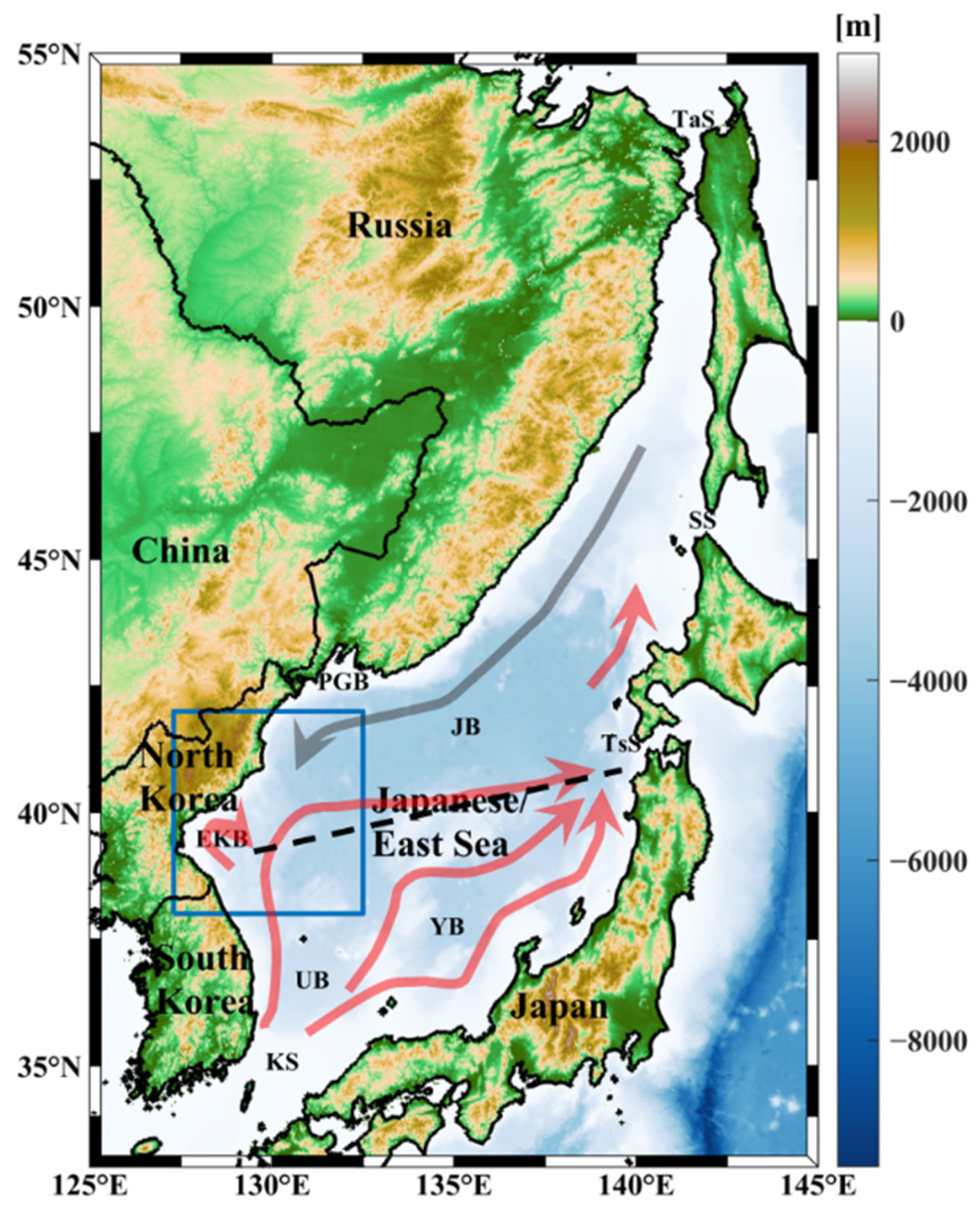
2. Data and Methods
2.1. Data
2.1.1. Observational Satellite Remote Sensing Data
2.1.2. Reanalysis Data
2.2. Methods
2.2.1. Definition of Marine Heatwaves
2.2.2. Area-Weighted
2.2.3. Oceanic Heat Flux across Boundaries of the Study Area
3. Results
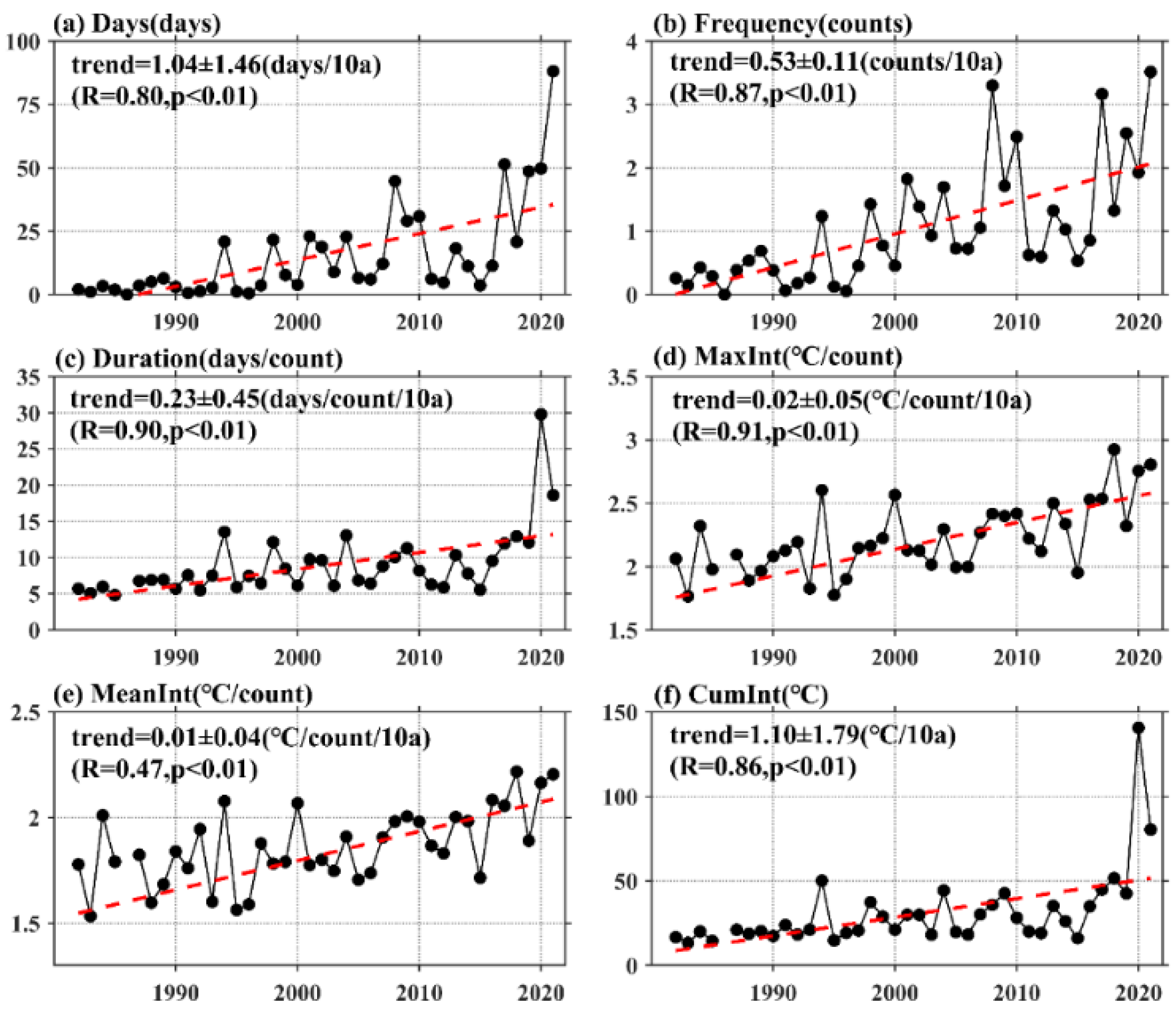
3.1. 1982–2021. MHWs Statistical Analysis
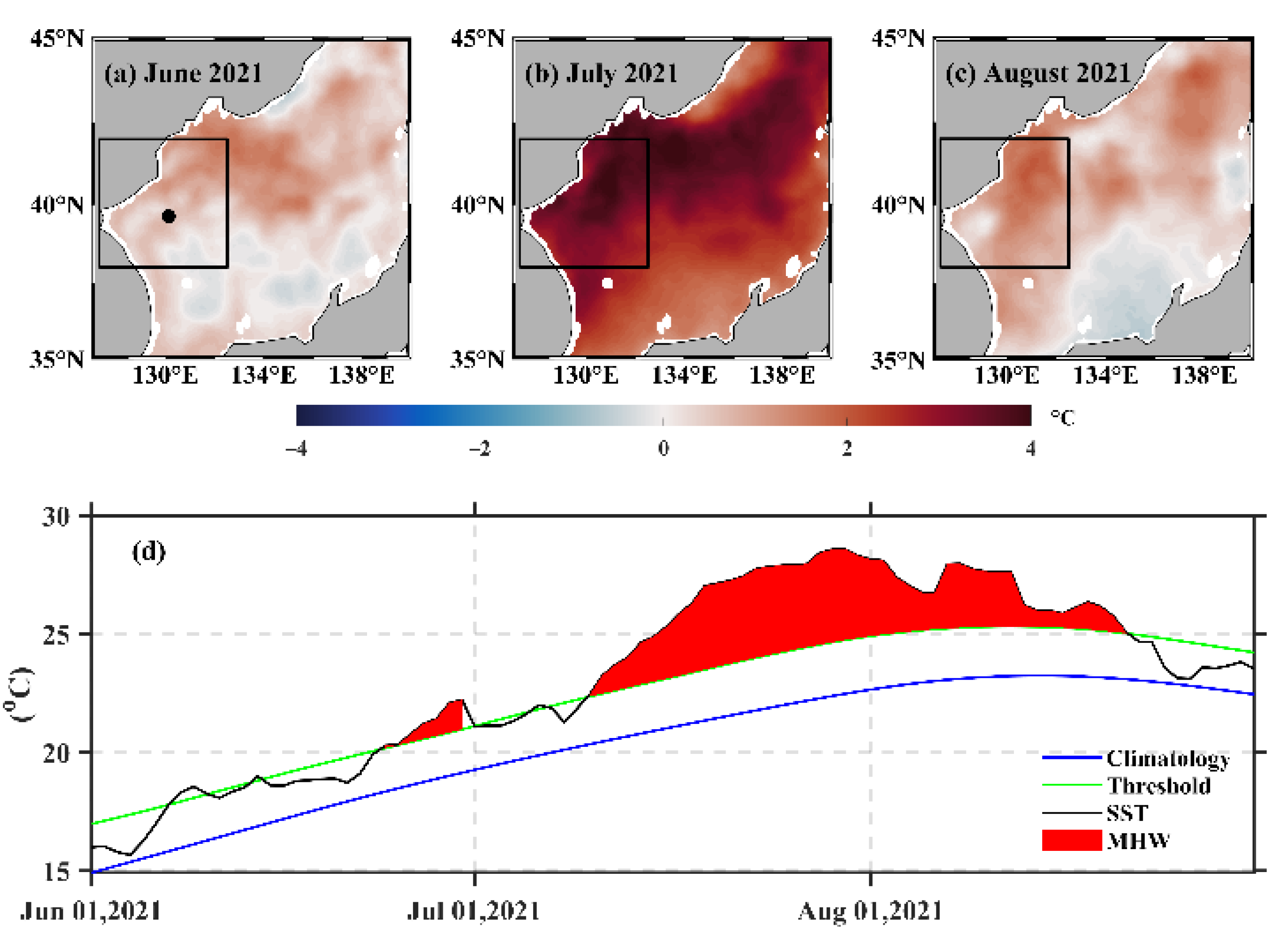
3.2. Analysis of MHW Events in the EKB in the Summer of 2021
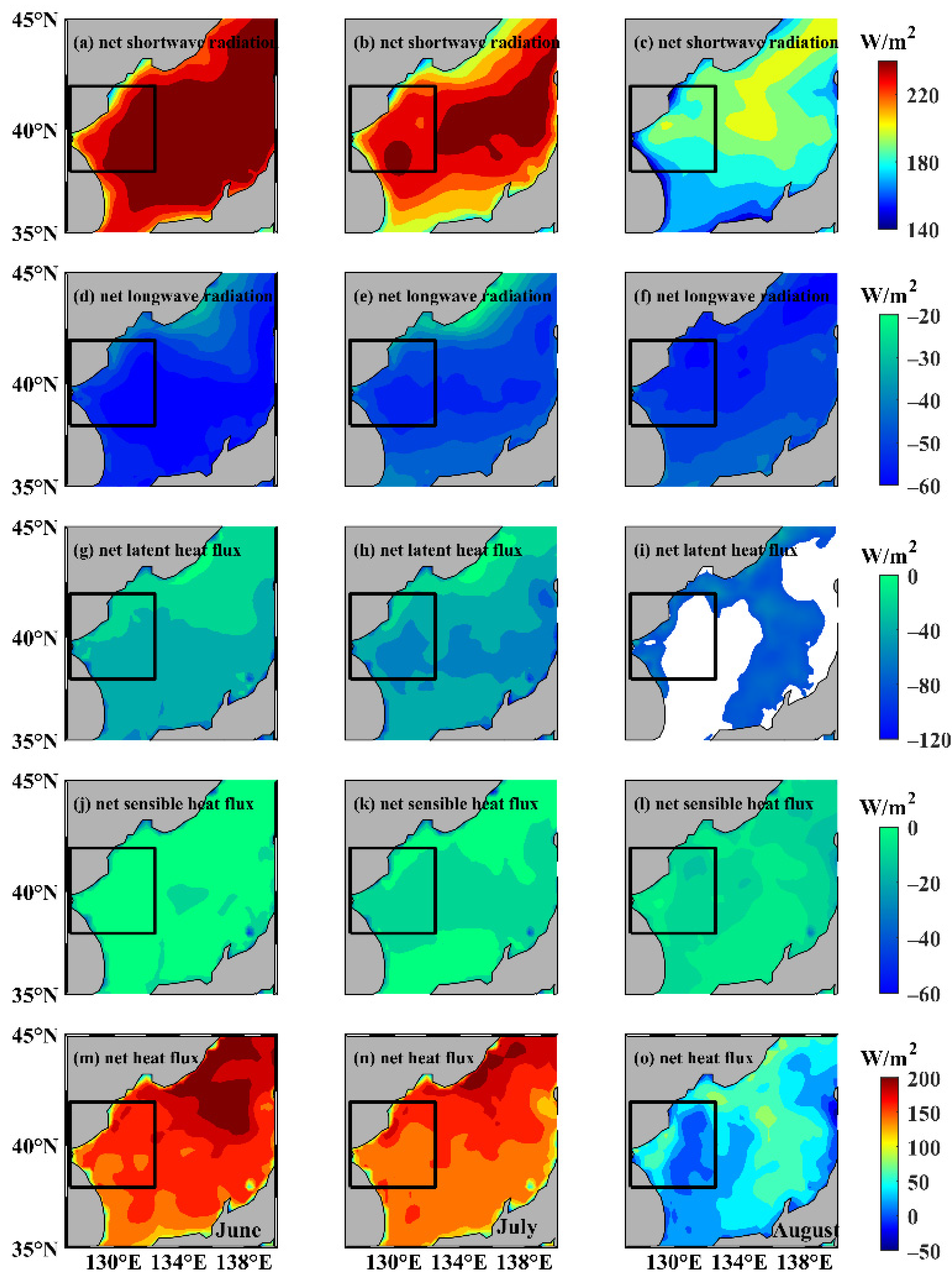
3.3. Driving Mechanisms for MHW Events in the EKB in the Summer of 2021
3.3.1. Vertical Heat Flux at the Sea Surface
3.3.2. Lateral Heat Fluxes from Open Boundaries
3.3.3. Effects of the Vertical Mixing
4. Discussion
4.1. Effects of Mesoscale Eddies
4.2. Potential Ecological Impacts
5. Conclusions
- (1)
- From 1982 to 2021, except for the Frequency, other MHW indices occur strongly in the western and central JES, especially in the EKB area, with rapidly increasing trends (p < 0.01).
- (2)
- Severe MHW events in the EKB take place in the summer of 2021. A high Days spot (50–70 days) can be observed in the northern part of the EKB, and MeanInt reaches more than 4.5 °C in the southern EKB area. The total days and mean intensity of MHWs that occur in the EKB are 1.84 and 1.47 times more than those averaged in the JES, respectively.
- (3)
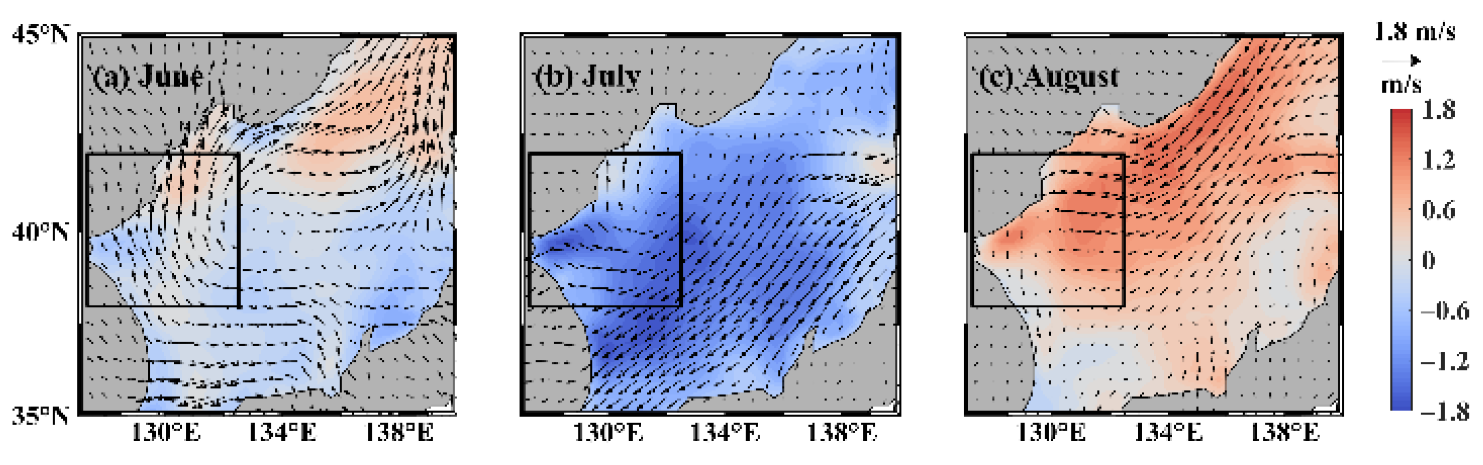
- The mechanisms for the occurrence of the MHWs in the summer of 2021 are primarily caused by the atmospheric high-pressure system moving to the EKB area resulting in strong solar radiation into the upper ocean and positive net heat flux. Other two reasons provide a condition for less water cooling: the net positive lateral heat fluxes across open boundaries, and the weak sea surface wind over the EKB area. The combination of the above three factors introduces the occurrences of the summer MHWs in the EKB in 2021.
Author Contributions
Funding
Data Availability Statement
Acknowledgments
Conflicts of Interest
References
- Cheng, L.; Trenberth, K.E.; Fasullo, J.; Boyer, T.; Abraham, J.; Zhu, J. Improved estimates of ocean heat content from 1960 to 2015. Sci. Adv. 2017, 3, e1601545. [Google Scholar] [CrossRef] [PubMed] [Green Version]
- Cheng, L.; Abraham, J.; Trenberth, K.E.; Fasullo, J.; Boyer, T.; Locarnini, R.; Zhang, B.; Yu, F.; Wan, L.; Chen, X.; et al. Upper Ocean Temperatures Hit Record High in 2020. Adv. Atmos. Sci. 2021, 38, 1–8. [Google Scholar] [CrossRef]
- Pörtner, H.-O.; Roberts, D.C.; Masson-Delmotte, V.; Zhai, P.; Tignor, M.; Poloczanska, E.; Weyer, N. IPCC Special Report on the Ocean and Cryosphere in a Changing Climate; IPCC Intergovernmental Panel on Climate Change: Geneva, Switzerland, 2019; p. 1. [Google Scholar]
- Pearce, A.; Lenanton, R.C.; Jackson, G.; Moore, J.; Feng, M.; Gaughan, D.J. The “marine heat wave” off Western Australia during the summer of 2010/11. Fish. Res. Rep. 2011, 222. [Google Scholar]
- Hobday, A.J.; Alexander, L.V.; Perkins, S.E.; Smale, D.A.; Straub, S.C.; Oliver, E.C.; Benthuysen, J.A.; Burrows, M.T.; Donat, M.G.; Feng, M.; et al. A hierarchical approach to defining marine heatwaves. Prog. Oceanogr. 2016, 141, 227–238. [Google Scholar] [CrossRef] [Green Version]
- Oliver, E.C.J.; Donat, M.G.; Burrows, M.T.; Moore, P.J.; Smale, D.A.; Alexander, L.V.; Benthuysen, J.A.; Feng, M.; Sen Gupta, A.; Hobday, A.J.; et al. Longer and more frequent marine heatwaves over the past century. Nat. Commun. 2018, 9, 1324. [Google Scholar] [CrossRef] [PubMed] [Green Version]
- Holbrook, N.J.; Gupta, A.S.; Oliver, E.C.; Hobday, A.J.; Benthuysen, J.A.; Scannell, H.A.; Smale, D.A.; Wernberg, T. Keeping pace with marine heatwaves. Nat. Rev. Earth Environ. 2020, 1, 482–493. [Google Scholar] [CrossRef]
- Oliver, E.C.; Benthuysen, J.A.; Darmaraki, S.; Donat, M.G.; Hobday, A.J.; Holbrook, N.J.; Schlegel, R.W.; Gupta, A.S. Marine heatwaves. Annu. Rev. Mar. Sci. 2020, 13. [Google Scholar] [CrossRef]
- Frölicher, T.L.; Fischer, E.M.; Gruber, N. Marine heatwaves under global warming. Nature 2018, 560, 360–364. [Google Scholar] [CrossRef]
- Oliver, E.C.; Burrows, M.T.; Donat, M.G.; Sen Gupta, A.; Alexander, L.V.; Perkins-Kirkpatrick, S.E.; Benthuysen, J.A.; Hobday, A.J.; Holbrook, N.J.; Moore, P.J. Projected marine heatwaves in the 21st century and the potential for ecological impact. Front. Mar. Sci. 2019, 6, 734. [Google Scholar] [CrossRef] [Green Version]
- Holbrook, N.J.; Scannell, H.A.; Gupta, A.S.; Benthuysen, J.A.; Feng, M.; Oliver, E.C.; Alexander, L.V.; Burrows, M.T.; Donat, M.G.; Hobday, A.J.; et al. A global assessment of marine heatwaves and their drivers. Nat. Commun. 2019, 10, 2624. [Google Scholar] [CrossRef] [Green Version]
- Bond, N.A.; Cronin, M.F.; Freeland, H.; Mantua, N. Causes and impacts of the 2014 warm anomaly in the NE Pacific. Geophys. Res. Lett. 2015, 42, 3414–3420. [Google Scholar] [CrossRef]
- Rodrigues, R.R.; Taschetto, A.S.; Sen Gupta, A.; Foltz, G.R. Common cause for severe droughts in South America and marine heatwaves in the South Atlantic. Nat. Geosci. 2019, 12, 620–626. [Google Scholar] [CrossRef]
- Amaya, D.J.; Alexander, M.A.; Capotondi, A.; Deser, C.; Karnauskas, K.B.; Miller, A.J.; Mantua, N.J. Are long-term changes in mixed layer depth influencing North Pacific marine heatwaves? Bull. Am. Meteorol. Soc. 2021, 102, S59–S66. [Google Scholar] [CrossRef]
- Feng, M.; Mcphaden, M.J.; Xie, S.; Hafner, J. La Niña forces unprecedented Leeuwin Current warming in 2011. Sci. Rep. 2013, 3, 1277. [Google Scholar] [CrossRef] [PubMed] [Green Version]
- Gao, G.; Marin, M.; Feng, M.; Ding, Y.; Song, D. Drivers of Marine Heatwaves in the East China Sea and the South Yellow Sea in Three Consecutive Summers During 2016–2018. J. Geophys. Res. Ocean. 2020, 125, e2020JC016518. [Google Scholar] [CrossRef]
- Kuroda, H.; Setou, T. Extensive Marine Heatwaves at the Sea Surface in the Northwestern Pacific Ocean in Summer 2021. Remote Sens. 2021, 13, 3989. [Google Scholar] [CrossRef]
- Yao, Y.; Wang, J.; Yin, J.; Zou, X. Marine heatwaves in China’s marginal seas and adjacent offshore waters: Past, Present, and Future. J. Geophys. Res. Ocean. 2020, 125, e2019JC015801. [Google Scholar] [CrossRef]
- Wang, D.; Xu, T.; Fang, G.; Jiang, S.; Wang, G.; Wei, Z.; Wang, Y. Characteristics of Marine Heatwaves in the Japan/East Sea. Remote Sens. 2022, 14, 936. [Google Scholar] [CrossRef]
- Wang, H.; Chen, S.; Wang, N.; Yu, P.; Yang, X.; Wang, Y.; Zhang, Y. Evaluation of multi-model current data in the East/Japan Sea. In Proceedings of the 2020 3rd IEEE International Conference on Information Communication and Signal Processing (ICICSP 2020), Shanghai, China, 12–15 December 2020; pp. 486–491. [Google Scholar]
- Cai, R.; Tan, H.; Kontoyiannis, H. Robust surface warming in offshore China seas and its relationship to the east Asian monsoon wind field and ocean forcing on interdecadal time scales. J. Clim. 2017, 30, 8987–9005. [Google Scholar] [CrossRef]
- Huang, B.; Liu, C.; Banzon, V.; Freeman, E.; Graham, G.; Hankins, B.; Smith, T.; Zhang, H.-M. Improvements of the Daily Optimum Interpolation Sea Surface Temperature (DOISST) Version 2.1. J. Clim. 2020, 34, 2923–2939. [Google Scholar] [CrossRef]
- Chelton, D.B.; Schlax, M.G.; Samelson, R.M.; de Szoeke, R.A. Global observations of large oceanic eddies. Geophys. Res. Lett. 2007, 34, L15606. [Google Scholar] [CrossRef]
- Chelton, D.B.; Schlax, M.G.; Samelson, R.M. Global observations of nonlinear mesoscale eddies. Prog. Oceanogr. 2011, 91, 167–216. [Google Scholar] [CrossRef]
- Oliver, E.; Benthuysen, J.; Bindoff, N.; Hobday, A.J.; Holbrook, N.J.; Mundy, C.N.; Perkins-Kirkpatrick, S.E. The unprecedented 2015/16 Tasman Sea marine heatwave. Nat. Commun. 2017, 8, 16101. [Google Scholar] [CrossRef] [PubMed] [Green Version]
- Zhao, Z.; Marin, M. A MATLAB toolbox to detect and analyze marine heatwaves. J. Open Source Softw. 2019, 4, 1124. [Google Scholar] [CrossRef]
- Yao, Y.; Wang, C. Variations in summer marine heatwaves in the South China Sea. J. Geophys. Res. Ocean. 2021, 126, e2021JC017792. [Google Scholar] [CrossRef]
- Zhao, N.; Manda, A.; Han, Z. Frontogenesis and frontolysis of the subpolar front in the surface mixed layer of the Japan Sea. J. Geophys. Res. Ocean. 2014, 119, 1498–1509. [Google Scholar] [CrossRef] [Green Version]
- Black, E.; Blackburn, M.; Harrison, G.; Hoskins, B.; Methven, J. Factors contributing to the summer 2003 European heatwave. Weather 2004, 59, 217–223. [Google Scholar] [CrossRef]
- Lee, T.; Hobbs, W.R.; Willis, J.K.; Halkides, D.; Fukumori, I.; Armstrong, E.M.; Hayashi, A.K.; Liu, W.T.; Patzert, W.; Wang, O. Record warming in the South Pacific and western Antarctica associated with the strong central-Pacific El Niño in 2009–10. Geophys. Res. Lett. 2010, 37, L19704. [Google Scholar] [CrossRef] [Green Version]
- Choi, W.; Bang, M.; Joh, Y.; Ham, Y.-G.; Kang, N.; Jang, C.J. Characteristics and Mechanisms of Marine Heatwaves in the East Asian Marginal Seas: Regional and Seasonal Differences. Remote Sens. 2022, 14, 3522. [Google Scholar] [CrossRef]
- Feng, Y.; Bethel, B.J.; Dong, C.; Zhao, H.; Yao, Y.; Yu, Y. Marine heatwave events near Weizhou island, beibu gulf in 2020 and their possible relations to coral bleaching. Sci. Total Environ. 2022, 823, 153–414. [Google Scholar] [CrossRef] [PubMed]
- Shin, H.; Lee, J.; Kim, C.; Yoon, J.H.; Hirose, N.; Takikawa, T.; Cho, K. Long-term variation in volume transport of the Tsushima warm current estimated from ADCP current measurement and sea level differences in the Korea/Tsushima Strait. J. Mar. Syst. 2022, 232, 103750. [Google Scholar] [CrossRef]
- Ansorge, I.J.; Jackson, J.M.; Reid, K.; Durgadoo, J.V.; Swart, S.; Eberenz, S. Evidence of a southward eddy corridor in the South-West Indian ocean. Deep. Sea Res. Part II Top. Stud. Oceanogr. 2015, 119, 69–76. [Google Scholar] [CrossRef]
- Dong, C.M.; McWilliams, J.C.; Liu, Y.; Chen, D. Global heat and salt transports by eddy movement. Nat. Commun. 2014, 5, 1–6. [Google Scholar] [CrossRef] [PubMed] [Green Version]
- Joo, H.T.; Park, J.W.; Son, S.H.; Noh, J.H.; Jeong, J.Y.; Kwak, J.H.; Saux-Picart, S.; Choi, J.H.; Kang, C.K.; Lee, S.H. Long-term annual primary production in the Ulleung Basin as a biological hot spot in the East/Japan Sea. J. Geophys. Res. Ocean. 2014, 119, 3002–3011. [Google Scholar] [CrossRef]
- Kida, S.; Takayama, K.; Sasaki, Y.N.; Matsuura, H.; Hirose, N. Increasing trend in Japan Sea Throughfow transport. J. Oceanogr. 2020, 77, 145–153. [Google Scholar] [CrossRef]


| Index | Unit | 2008 | 2017 | 2018 | 2019 | 2020 | 2021 |
| Days | Days | 29.16 | 33.11 | 23.02 | 46.28 | 55.03 | 90.14 |
| Frequency | Counts | 2.66 | 2.70 | 1.81 | 3.34 | 2.92 | 4.67 |
| Duration | Days/count | 7.87 | 8.32 | 10.36 | 9.07 | 16.84 | 14.84 |
| MaxInt | °C/count | 2.11 | 2.03 | 2.30 | 1.95 | 2.10 | 2.34 |
| MeanInt | °C/count | 1.72 | 1.70 | 1.85 | 1.60 | 1.68 | 1.85 |
| CumInt | °C | 18.78 | 20.00 | 27.16 | 20.20 | 48.11 | 41.32 |
Disclaimer/Publisher’s Note: The statements, opinions and data contained in all publications are solely those of the individual author(s) and contributor(s) and not of MDPI and/or the editor(s). MDPI and/or the editor(s) disclaim responsibility for any injury to people or property resulting from any ideas, methods, instructions or products referred to in the content. |
© 2023 by the authors. Licensee MDPI, Basel, Switzerland. This article is an open access article distributed under the terms and conditions of the Creative Commons Attribution (CC BY) license (https://creativecommons.org/licenses/by/4.0/).
Share and Cite
Chen, S.; Yao, Y.; Feng, Y.; Zhang, Y.; Xia, C.; Sian, K.T.C.L.K.; Dong, C. Characteristics and Drivers of Marine Heatwaves in 2021 Summer in East Korea Bay, Japan/East Sea. Remote Sens. 2023, 15, 713. https://doi.org/10.3390/rs15030713
Chen S, Yao Y, Feng Y, Zhang Y, Xia C, Sian KTCLK, Dong C. Characteristics and Drivers of Marine Heatwaves in 2021 Summer in East Korea Bay, Japan/East Sea. Remote Sensing. 2023; 15(3):713. https://doi.org/10.3390/rs15030713
Chicago/Turabian StyleChen, Sijie, Yulong Yao, Yuting Feng, Yongchui Zhang, Changshui Xia, Kenny T. C. Lim Kam Sian, and Changming Dong. 2023. "Characteristics and Drivers of Marine Heatwaves in 2021 Summer in East Korea Bay, Japan/East Sea" Remote Sensing 15, no. 3: 713. https://doi.org/10.3390/rs15030713