Abstract
Landmines and explosive remnants of war are a significant threat in tens of countries and other territories, causing the deaths or injuries of thousands of people every year, even long after military conflicts. Effective technical means of remote detecting, localizing, imaging, and identifying mines and other buried explosives are still sought and have a great potential utility. This paper considers a positioning system used as a supporting tool for a handheld ground penetrating radar. Accurate knowledge of the radar antenna position during terrain scanning is necessary to properly localize and visualize the shape of buried objects, which helps in their remote classification and makes demining safer. The positioning system proposed in this paper uses ultrawideband radios to measure the distances between stationary beacons and mobile units. The measurements are processed with an extended Kalman filter based on an innovative dynamics model, derived from the model of a pendulum motion. The results of simulations included in the paper prove that using the proposed pendulum dynamics model ensures a better accuracy than the accuracy obtainable with other typically used dynamics models. It is also demonstrated that our positioning system can estimate the radar antenna position with the accuracy of single centimeters which is required for appropriate imaging of buried objects with the ground penetrating radars.
1. Introduction
The presence of landmines and explosive remnants of war (ERW), such as artillery shells, grenades, rockets, bombs, and cluster munition remnants, poses a significant worldwide threat in the areas of current and past military conflicts. It results in deaths and injuries of mostly civilian victims even many years after the wars.
According to the yearly reports of the Landmine Monitor [1,2], providing a global overview of the landmine situation, tens of millions of landmines are still buried underground in at least 60 countries and other territories. Only a single year 2021 brought 7073 casualties of mines/ERW (2492 killed and 4561 injured) in 54 different countries, and 80% of the victims were civilians [1,2,3].
Considering the significance of the problem, efficient methods of mine clearance are still tough. Currently, various metal detectors (MD) are often used for this purpose, and contemporary MDs offer excellent parameters, enabling the detection of even very small and deeply buried metal objects [4,5,6,7,8,9]. Paradoxically, this high sensitivity can be also their drawback leading to many false detections which lengthen the time necessary for demining. Moreover, MDs do not offer any way to initially identify or classify the detected objects and every detection must be carefully examined. What is even more problematic and dangerous, not all contemporary landmines and ERWs contain metal elements, which limits the usefulness of MDs in mine clearance operations.
Apart from the MDs, radar technology has been successfully employed for scanning near-underground surfaces in search of mines, improvised explosive devices (IED), and other explosive remnants of war [6,7,8,10,11,12,13,14]. Ground penetrating radar (GPR) is a general term used with respect to techniques using radio waves, typically in a frequency range from several MHz to several GHz, to acquire information about objects buried underground or hidden under/behind any other concealing obstacles, surfaces, etc. [3,15,16,17,18,19,20,21]. These techniques enable non-invasive and non-destructive remote detecting, locating, imaging, and identifying geological structures, cavities, buried objects, and underground man-made infrastructures, which do not have to contain metal parts. The mentioned features make GPRs a very useful tool for demining. They can be used for this purpose alone [12,17,22,23,24] or integrated with MDs [12,25,26,27,28,29,30].
In military applications, GPRs can be installed on large armored manned vehicles with enhanced immunity to nearby explosions [31,32,33,34,35]. For increased safety of the crew, the radar antennas are usually attached to the end of long arms in front of the vehicle. A good alternative is mounting GPRs on remotely controlled unmanned wheeled vehicles [36] or tracked vehicles [30,35,37,38], which eliminates the risk for the crew, and reduces the costs of the purchase and the exploitation of such systems. The GPRs on vehicle platforms, however, have limited utility in difficult terrain: mountainous areas, forests, dumps, urban surfaces covered with debris, or interiors of buildings, where landmines and other explosives can be typically found. A good solution applicable in such areas is a handheld version of the ground penetrating radar (HH-GPR) [39,40,41,42]. The problem of estimating the antenna position of such type of radar is addressed in this paper.
The GPR operation requires emitting electromagnetic energy in the direction of the ground. The transmitted radio waves penetrate near-surface layers of the soil and encounter on their way various objects and layers of different permittivity and conductivity , which results in reflecting and scattering back a portion of the transmitted energy. The echo signals are received, collected, and processed to detect and create images of buried objects.
Most contemporary GPRs are pulse radars [15,16,22,24,43,44], transmitting repeatable, very short, high-amplitude pulses and receiving strongly attenuated echo signals reflected or scattered back from layers’ boundaries and buried objects [3,45,46] as shown in Figure 1.
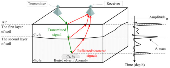
Figure 1.
General idea of GPR operation.
Time delays of subsequent peaks in the received echo signals are proportional to the depth of the detected objects or layers of different permittivity. Collecting and joint processing multiple echo signals, so-called echograms or radargrams, for a GPR moving along a predefined scanning path enables locating and imaging those objects and layers [3,15,16].
Three types of visual presentations of GPR radargrams are used in practice [3,14,16,21]. A single echogram was obtained for only one GPR antenna position with coordinates is a one-dimensional signal representation, called an A-scan (Figure 2a). Time delays of the signal peaks in the A-scan are usually converted into respective depths and the Z-axis is scaled in the distance units [21,23,39,46,47].
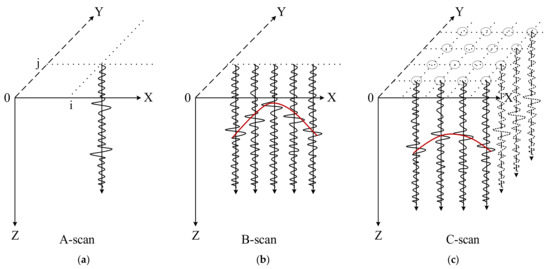
Figure 2.
Types of GPR radargrams’ visual presentations: (a) A-scan; (b) B-scan; (c) C-scan.
An analysis of GPR data is typically based on a two-dimensional signal representation, called a B-scan, which is a dataset created from many A-scans acquired for various antenna locations along a usually linear scanning path, as shown in Figure 2b. It represents a radar image of a vertical surface intersecting the scanned terrain volume below the scanning path. Due to a relatively large GPR antenna beamwidth, the same buried objects are illuminated many times from different antenna locations and consequently from different distances. Therefore, the echo signals form hyperbolic structures visible in the B-scans [14,23,39,46,47]. An example of such a structure for a single-point object is shown as a red hyperbole in Figure 2b.
Collecting A-scans for multiple antenna locations in the nodes of a grid span onto the surface, one can create another type of GPR signal visual presentation, called a C-scan (Figure 2c). This is a three-dimensional signal representation, which is very useful in visualizing, identifying, and classifying buried objects.
The C-scans are often presented as a set of two-dimensional greyscale or color images, created as horizontal sections through the C-scan volume on various depths [3,21,48]. An example of such a single image is shown in Figure 3.
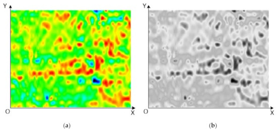
Figure 3.
Examples of a horizontal section through a C-scan: (a) color image; (b) grayscale image.
The presented scans were made using a pulse radar produced by IDS GeoRadar company, containing a DAD K2 control unit and an antenna with a central frequency equal to . This radar made 850 soundings per second, the duration of the probing pulse was about 1 ns, and the obtained spatial resolution was about .
Knowledge of accurate positions of a GPR antenna moving along a scanning path is necessary to properly assemble all the acquired radargrams and create high-quality GPR B-scans or C-scans. Several scientific papers [44,49] and patents [50] suggest that the GPR antenna positioning accuracy should be better than one eight of a radar signal wavelength [51]. As typical GPRs work at a frequency range between and (wavelengths from to ) [49,51], the antenna positioning accuracy should be of the order of single centimeters which requires using very high-accuracy navigation systems.
Typically, the navigation devices or systems used for GPR antenna positioning are Global Navigation Satellite Systems (GNSS) receivers [50,52], often with real-time kinematic (RTK) corrections, inertial navigation systems [42,52], wheel odometers [50], visual navigation systems [53], laser scanners [49] or integrated systems combining several of the mentioned devices [42,50,52].
As most of the listed above devices or systems are not adequate for HH-GPRs, due to their large size, weight, specific installation requirements, vulnerability to jamming or signal shadowing, and too low accuracy, the authors of this paper proposed a system based on several ultrawideband (UWB) radio modules. This concept was first described in an authors’ conference paper [54], where physical models of a mobile unit and UWB beacons were presented. The mentioned paper also contained a description of an autocalibration procedure, used for self-locating the UWB beacons for quickly establishing a frame of reference before the scanning process, and presented an initial assessment of the system’s accuracy which in the scanning zone reaches desired level of 2–3 cm.
In another authors’ conference paper [41], it was claimed and demonstrated that the accuracy of the UWB positioning system can be further improved with a properly chosen estimation algorithm. In that paper, using an extended Kalman filter (EKF) based on a GPR antenna motion model, derived from the mathematical pendulum motion model, was proposed. The mentioned paper, however, contained a proof of concept rather than a complete and applicable positioning solution, as the proposed pendulum-based dynamics model used in the EKF was oversimplified to present the main idea only. It assumed that the attachment point of the “pendulum”, which is the position of a GPR operator’s arm, is initially known and that the angle of orientation of the main axis of the scanning section always equals zero degrees. These assumptions can hardly be met in practice. Moreover, the mentioned conference paper contained only a sketch of the system’s model and very limited results of its simulative testing.
This paper can be considered a significantly extended version of the above-mentioned conference paper. It presents an elaborated, practically applicable version of the GPR antenna positioning system using UWB radio modules and includes a complete description of its extended mathematical model and detailed results of its simulative testing. The main novelty of this paper includes:
- Elaboration and detailed presentation of an advanced and practically applicable dynamics and observation model of the UWB-based GPR antenna positioning system, with relinquished simplifying assumptions of the model presented in [41];
- Elaboration and detailed presentation of the estimation algorithm used in the proposed GPR antenna positioning system;
- Presentation of new and detailed results of simulative tests of the positioning system for various realistic system configurations.
This paper is organized as follows. A general concept of the ground penetrating radar, types of GPR data visualizations, accuracy requirements for GPR antenna positioning, technologies used for GPR positioning, previous authors’ works in this field, and a discussion of the novelty of this paper are presented in Section 1. The system’s description, its mathematical model, and the estimation algorithm elaborated by the authors are presented in Section 2. The methodology and the results of simulative testing of the GPR antenna positioning system are presented in Section 3 and Section 4 contain a discussion.
2. Materials and Methods
2.1. Scanning Profiles
As has already been mentioned, creating B-scans requires moving a GPR antenna over the ground, ideally along a linear scanning path (profile) with constant velocity, to collect linearly arranged and uniformly separated radargrams. Creating C-scans requires repeating such scanning (profiling) for many equidistant lines in one direction, as shown in Figure 4a, or bi-directionally, as shown in Figure 4b, where the antenna position is marked as a letter A [7,15,16]. In multichannel GPRs, with several equidistant antennas, the profiling can be realized quicker, unidirectionally (like in Figure 4a) for several scanning paths at a time.
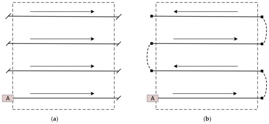
Figure 4.
Ideal GPR scanning profiles: (a) unidirectional; (b) bidirectional.
Although in favorable conditions the profiling shown in Figure 4 can be at least approximately realized with GPRs installed on vehicles (carefully driven or remotely controlled, in non-demanding terrain and with the use of an accurate supporting navigation system), this can hardly be achieved with HH-GPRs. The elements of the scanning path, in this case, are shown in Figure 5, where the letters A and S represent the positions of the antenna and the sapper.
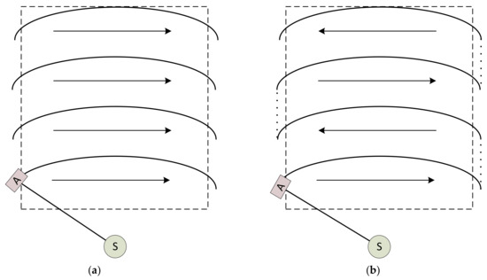
Figure 5.
Scanning profiles typical for HH-GPR: (a) unidirectional; (b) bidirectional.
2.2. UWB Positioning System
The structure of the HH-GPR antenna positioning system proposed in this paper is shown in Figure 6. It is composed of four stationary modules serving as radio beacons and two mobile modules and . The module is installed over the GPR antenna and the module over the sapper’s shoulder. All the modules contain UWB transceivers. Distance measurements realized by these transceivers are collected and processed using estimation algorithms described in the further part of the paper.
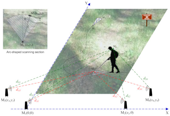
Figure 6.
UWB positioning system for HH-GPR antenna.
The following variables are used in Figure 6:
- —distance between a j-th beacon and the antenna module ,
- —distance between a j-th beacon and the sapper module ,
- —coordinates of a j-th beacon position,
- —coordinates of the module position,
- —coordinates of the module position,
- —length of the HH-GPR handle (horizontal distance between and ),
- —angle between the horizontal projection of the GPR antenna handle and the central axis of the scanning section.
We assumed that the UWB radios used in our system are PulsON P440 modules from TDSR [55]. They use the two-way time-of-flight (TW-TOF) method for ranging and offer an operating range between 300 and 1100 m and a ranging accuracy of about 2 cm in line of sight (LOS) conditions. Such parameters give the potential to build a positioning system with the desired centimeter-level accuracy, required in the considered application of the HH-GPR antenna positioning.
The placement of beacons outside a potentially hazardous area, as shown in Figure 6, is only one of the possible options, suggested for quick and easy deployment of the system in terrain. Other beacons’ locations are also possible, and their relative positions with respect to the mobile units and influence the accuracy of the UWB positioning system, which will be discussed in detail in the Results section of the paper.
2.3. Mathematical Model
As can be seen in Figure 5, the scanning profiles are composed of fragments that resemble arcs rather than straight sections. Moreover, the velocity of the HH-GPR antenna is more changeable than in GPRs installed on vehicle platforms, as typically an operator (sapper) performs a swinging motion, initially accelerating and finally decelerating the antenna. Therefore, the collected radargrams are not linearly arranged nor uniformly separated. Nevertheless, the acquired A-scans can be used to create two- or three-dimensional GPR visualizations of buried objects provided that the antenna positions are known for all the collected radargrams [3,15,16].
A single arc belonging to the scanning profile is shown in Figure 7. If we consider the changeable angular velocity of the antenna motion (initially accelerating and finally decelerating), such a trajectory resembles the motion of a mathematical pendulum [56], and can be described by the following formula:
where:
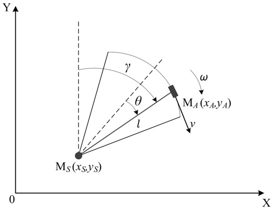
Figure 7.
Part of HH-GPR antenna trajectory (a single arc of the scanning profile).
—angle between the horizontal projection of the GPR antenna handle and the central axis of the scanning section,
—acceleration forcing the HH-GPR antenna ( module) motion,
—length of the HH-GPR handle (horizontal distance between and ).
The acceleration is analogous to the gravity acceleration in the mathematical pendulum motion model. Contrary to , which can be considered a constant, the acceleration is more changeable and to large extent depends on the operator’s strength, fatigue, style of HH-GPR operation, etc., thus we treat it as an additional variable to be estimated and we model it as a Wiener stochastic process [57,58,59]. Considering the geometrical relationships shown in Figure 7, the equations describing the antenna and the sapper’s arm motion can be formulated as follows:
where:
- —coordinates of the HH-GPR antenna ( module) position,
- —coordinates of the sapper’s arm ( module) position,
- —Gaussian white noises representing random components of the sapper’s arm ( module) motion,
- —length of the HH-GPR handle (horizontal distance between and ),
- —angle between the horizontal projection of the GPR antenna handle and the central axis of the scanning section,
- —angle between the horizontal projection of the GPR antenna handle and the axis of the frame of reference,
- —angular velocity of the HH-GPR antenna ( module) motion,
- —acceleration forcing the HH-GPR antenna ( module) motion,
- —Gaussian white noise representing random changes of .
Rewriting Equation (2) to fit it into the standard form of a nonlinear continuous dynamics model [60,61,62,63]:
one obtains the following detailed version of this model, which has been further used in our estimation algorithm:
The nonlinear observation model in the following standard form [60,61,62]:
has been formulated assuming that at every step the UWB positioning system realizes four distance measurements between a j-th beacon and the antenna module :
and four distance measurements between a j-th beacon and the sapper module :
where:
- —distance between a j-th beacon and the antenna module ,
- —distance between a j-th beacon and the sapper module ,
- —coordinates of a j-th beacon position,
- —coordinates of the module position,
- —coordinates of the module position,
- —sapper’s arm height,
- —distance measuring errors for and modules.
A detailed version of the observation model, which has been further used in our estimation algorithm, is as follows:
As the antenna module is kept close to the soil during scanning, and the differences between slant distances and their horizontal projections are very small, we assumed that their altitude over the ground can be omitted in the observation model. On the other hand, the module is placed over the ground on the sapper’s arm, and its altitude is non-negligible. In our model, we assumed that it is constant, as its changes in the order of centimeters during the system’s operation can be neglected for typical distances from the UWB beacons, which are in the order of tens of meters. In a real system the altitude can be a settable constant, adjusted before using the system, based on the sapper’s height.
2.4. Estimation Algorithm
An extended Kalman filter for HH-GPR antenna position estimation was designed based on the previously described dynamics and observation models and its flowchart is shown in Figure 8.
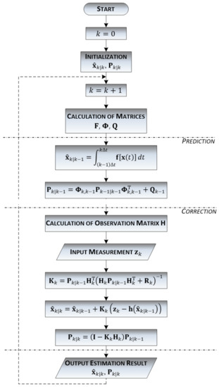
Figure 8.
Flowchart of the Extended Kalman Filter used for HH-GPR antenna position estimation.
After initialization of the EKF at step or after closing each subsequent filter’s loop at steps , the filter alternately performs prediction and correction steps. The prediction step requires previous calculations of the fundamental matrix , the transition matrix , and the covariance matrix of disturbances at every step . The method of calculating the matrix (more precisely it is but to shorten the notation the index will be omitted in further equations) is explained in Appendix A.
Using the calculated matrix and the matrix from the equation (4), and matrices are obtained as follows [60,61,62]:
where:
and is a period between two successive time steps and .
The matrix from Equation (11) represents the covariance matrix of continuous disturbances which is a 3-by-3 diagonal matrix containing power spectral densities of the noises composing the disturbances vector in Equation (4):
The predicted state vector is calculated in accordance with the following general equation [64,65]:
but in practical calculations we use Heun’s numerical integration method [65,66,67,68] which leads to the following formulae:
where is the final state vector estimate from the previous step .
Apart from the predicted state vector , the covariance matrix of prediction errors is calculated based on the covariance matrix of filtration errors from the previous step as follows [60,61,62]:
where we use the mentioned matrices and .
The correction step requires previous calculations of the observation matrix at every step , and the method of its calculation is explained in Appendix B. This step involves a calculation of the Kalman gains matrix , a correction of the predicted state vector based on the current measurement vector , which produces the final estimate at the step , as well as calculation the covariance matrix of filtration errors , and these operations are realized as follows [60,61,62]:
The matrix in Equation (16) is the covariance matrix of measurement errors [60,61] which is formed as an 8-by-8 diagonal matrix, containing the variances of all eight distance measurements performed between pairs of UWB modules in the positioning system:
where and represent variances of distance measurement between a j-th beacon and the antenna module or the sapper module .
2.5. Alternative Positioning Algorithms
Apart from the proposed pendulum-model-based EKF, simpler algorithms can also be used to estimate the HH-GPR antenna position. One possible solution is a non-linear least squares (NLS) algorithm [57,69,70] which processes a vector of distance measurements collected at each step without using the previously estimated state vector and without filtration. Such an algorithm does not use any dynamics model either. The NLS requires an initialization by assigning at least coarse values to the antenna coordinates and and subsequently, it improves their estimates iteratively. This algorithm is simple but due to lack of filtration, its accuracy is not high.
Better estimation results can be obtained by using EKF filters based on nearly-constant-velocity (CV) or nearly-constant-acceleration (CA) dynamics models [57,71,72,73,74], which are typically applied in navigation and radiolocation. The CV model (20) assumes a rectilinear uniform motion, whereas the CA model (21) assumes a uniformly accelerated motion, and, in both cases, small disturbances of these ideal movements are modeled by the vector :
where:
- —coordinates of antenna position,
- —components of antenna velocity,
- —components of antenna acceleration,
- —Gaussian white noises representing random disturbances of CV motion,
- —Gaussian white noises representing random disturbances of CA motion.
Clearly, the CV and CA models do not fit ideally the actual HH-GPR antenna motion but nevertheless, they can be used for prediction in EKFs. Such filters are not optimal, but they are simpler than the EKF presented in Figure 8 because both dynamics models are linear, and the prediction of the state vector is realized like in a linear Kalman filter [60,61,62]:
Moreover, the transition matrix and the covariance matrix of disturbances can be calculated in advance before the filter implementation using the simple formula [62] and they remain constant during the filters’ operation. Thus, such EKFs do not require in-run calculation of the Jacobian matrix and the matrices and .
All the mentioned algorithms, NLS and EKFs based on the CV and CA models, have been implemented by the authors and tested to compare them with the previously described pendulum-model-based EKF. Further in the paper, the following acronyms will be used for these algorithms: NLS, EKF-CV, EKF-CA, and EKF-PND.
Although the EKF-CV and the EKF-CA are not optimal, their accuracy can be maximized by choosing appropriate power spectral densities of disturbances of noises in the CV model or of noises in the CA model. Their choice affects the values of the matrices and consequently influences the information quality [75], notably estimation errors of the filters. The process of choosing filters’ parameters and minimizing their estimation errors is called “tuning Kalman filter” [76] and it was realized in the case of the EKF-CV and EKF-CA designed in our research.
3. Results
The described HH-GPR antenna positioning system and the proposed pendulum-model-based EKF were implemented and simulatively tested in MATLAB® version R2022b. The simulations included an assessment of the dependence of the system’s accuracy on the positions of UWB stationary modules deployed around the area of interest, where the demining process is going to be performed. The results of these analyses are presented in Section 3.1. In further experiments, the accuracy of the EKF-PND filter was analyzed for chosen scanning sections. This accuracy was also compared with the accuracy of the NLS, EKF-CV, and EKF-CA algorithms. The results of these tests and accuracy comparisons are presented in Section 3.2.
3.1. Influence of UWB Beacons’ Locations on System’s Accuracy
Possible locations of the UWB stationary modules are to large extent dependent on the terrain characteristics and the obstacles present around the scanning area. The sapper usually cannot place it freely when he deploys the system’s elements in a previously unsearched and potentially hazardous terrain. When approaching a minefield, he usually knows which part of the terrain is free of explosives and where the search should start. Thus, the most typical and safe locations for placing the UWB beacons lay in front and on the sides of the minefield, as shown in Figure 6. Such a system’s geometry is certainly not optimal from the accuracy point of view, but even under the mentioned limitations, the actual placement of may significantly influence the positioning accuracy in various areas of the minefield.
To verify the mentioned dependence of the positioning accuracy on the locations of the UWB stationary modules, three system configurations with different locations of the modules were considered. The assumed positions of the modules are given in Table 1 and are graphically presented in Figure 9.

Table 1.
Locations of the UWB stationary modules for different system configurations.
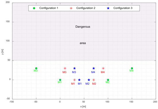
Figure 9.
Locations of the UWB stationary modules for different system configurations.
We assumed that an area of lying in front of the UWB beacons is divided by a grid with cells of each. For every node of this grid, a set of ten thousand UWB measurements was generated in MATLAB®, and its position was estimated using a simple iterative NLS algorithm, without any Kalman filtration. Based on the parameters of P440 modules, declared by their producer [55], we assumed that UWB measurement errors have zero-mean Gaussian distribution with a standard deviation of . Next, RMS errors (RMSE) for each node were calculated and the obtained results for the three system’s configurations are shown as colormaps in Figure 10. As the RMSE is very large in the vicinity of the UWB modules, the colormap is presented for the area where the coordinate is larger or equal to . In practice, it means that the actual placement of the UWB beacons should be in the foreground of the minefield, far enough ahead of its border, to ensure that the positioning accuracy in the planned search zone is high.
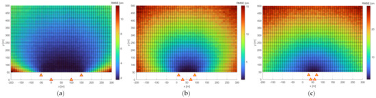
Figure 10.
RMSE for different system configurations: (a) C1; (b) C2; (c) C3.
As can be seen, the smallest positioning errors are achievable in front of the place, where the UWB stationary modules are located. The high-accuracy zone is wider and deeper for a more extended baseline of the positioning system.
Mean and maximal RMSE values for the whole area of and for smaller areas, limited to the nearest and respectively, in front of the UWB stationary modules are given in Table 2.
Table 2.
Mean and maximal RMSE values for areas of various sizes.
As can be seen, the proposed positioning system can provide a centimeter level of accuracy in areas large enough for practical demining tasks and for reasonable and practically realizable systems’ configurations. The high-accuracy zone could certainly be extended if the UWB stationary modules were more distributed around the area to be scanned, however for safety reasons it cannot always be achieved.
3.2. Positioning Accuracy
The accuracy of the EKF-PND filter was assessed and compared with the accuracy of EKF-CV and EKF-CA filters as well as with the accuracy of an NLS algorithm in MATLAB® for the C1 configuration of the system. The dynamics and observation models given by Equations (4) and (8) were used to generate the antenna trajectories and the parameters chosen during the simulations are given in Table 3. The choice of these parameters was done in such a way that the shape and duration of the resulting antenna trajectory resemble typical HH-GPR antenna trajectories.
Table 3.
Parameters used in dynamics and observation models during simulations.
The same standard deviations of all the distance measuring errors and power spectral densities given in Table 3 were used in the EKF-PND for setting the values of the and matrices. The EKF-CV and EKF-CA also use as given in Table 3, but as their dynamics models are different, their matrices required finding power spectral densities of different noises or . This was done during the mentioned tuning process and the obtained values are as follows: and .
Firstly, the results of the antenna position estimation with the EKF-PND and the NLS algorithm were compared for various orientations of scanning sections and chosen results of these tests are presented in Figure 11. These experiments confirmed that the EKF-PND filter works properly and achieves a similar accuracy for various orientations of the central axis of the scanning section.
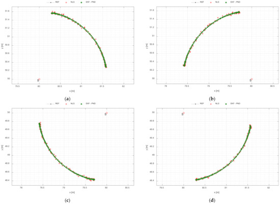
Figure 11.
Estimated antenna positions with EKF-PND and NLS, for various orientations of the central axis of the scanning section: (a) ; (b) ; (c) ; (d) .
Next, a closer inspection of the estimation results was done for all the implemented algorithms for a chosen orientation of the central axis of the scanning section equal to .
A comparison of HH-GPR antenna positions estimated with NLS, EKF-CV, EKF-CA, and EKF-PND is presented in Figure 12. As can be seen, all these algorithms are capable of properly estimating the antenna position, however, their accuracy is noticeably different and required further analysis, which will be presented further.
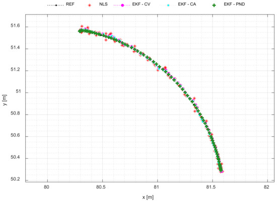
Figure 12.
Comparison of antenna positions estimated with NLS, EKF-CV, EKF-CA, and EKF-PND.
At this step of the simulations, the results of the estimation of other elements of the state vector from the dynamics model given by Equation (4) were analyzed and they are presented in Figure 13, Figure 14 and Figure 15. The angle between the horizontal projection of the antenna handle and the central axis of the scanning section, estimated with the EKF-PND filter, is shown in Figure 13. The results of angular velocity estimation are presented in Figure 14. Figure 15 contains an estimate of the acceleration forcing the HH-GPR antenna movement. All these figures contain only results for the EKF-PND, as other algorithms do not estimate variables such as , and .
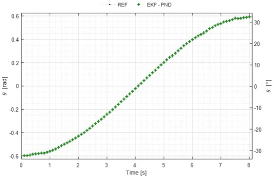
Figure 13.
Angle between the horizontal projection of the antenna handle and the central axis of the scanning section estimated with EKF-PND.
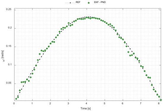
Figure 14.
Angular velocity of the antenna motion estimated with EKF-PND.
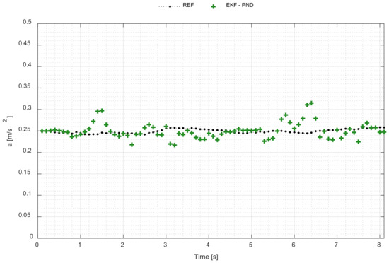
Figure 15.
Acceleration estimated with EKF-PND.
To better compare the accuracy of estimation with various algorithms, we conducted a series of ten thousand simulations and calculated average RMS antenna position errors for the whole scanning sections for each realization of the simulations. The obtained RMSE values are shown in Figure 16. Single points in various colors are RMS antenna position errors obtained with NLS, EKF-CV, EKF-CA, and EKF-PND. Although they are changeable in various simulation runs, they form bands on noticeably different levels.
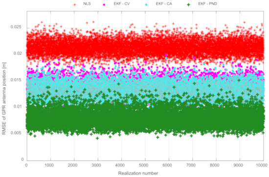
Figure 16.
Comparison of RMS antenna position errors for NLS, EKF-CV, EKF-CA, and EKF-PND.
Based on the above results we created a histogram of RMS antenna position errors for NLS, EKF-CV, EKF-CA, and EKF-PND and it is presented in Figure 17. From this and the previous figure, one can conclude that the EKF-PND is more accurate than all other tested algorithms and the EKF-CV and EKF-CA perform similarly, but still better than the NLS algorithm. The EKF-CA is slightly more accurate than the EKF-CV.
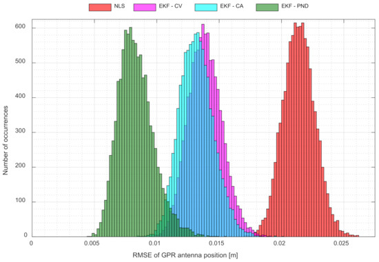
Figure 17.
Histogram of RMS antenna position errors for NLS, EKF-CV, EKF-CA, and EKF-PND.
A comparison of numerical values of average RMS antenna position errors for all the realizations and for the NLS, EKF-CV, EKF-CA, and EKF-PND algorithms are given in Table 4. This table also presents percentage improvements of accuracy for EKF-CV and EKF-CA vs. NLS and EKF-PND versus all other algorithms. As can be seen, in the chosen simulation scenario, the EKF-PND provides positioning results about 40% more accurate than other tested EKFs and about 60% better than NLS.
Table 4.
Average RMS antenna position errors for NLS, EKF-CV, EKF-CA, and EKF-PND.
4. Discussion
In this paper, an accurate positioning system dedicated as a supporting tool for a handheld ground penetrating radar was presented. The system uses ultrawideband radio technology for accurate distance measurements and processes them to estimate the GPR antenna position. Various estimation algorithms were used for this purpose, from NLS, through simple EKFs (EKF-CV and EKF-CA), based on those typically used in radiolocation and navigation CV and CA dynamics models, to the EKF-PND, based on the proposed by the authors’ dynamics model derived from the model of a pendulum motion.
The results of simulations included in the paper have demonstrated that the proposed positioning system can provide a desired centimeter level of accuracy in areas large enough for practical demining tasks. They also have shown how the actual placement of UWB beacons influences the system’s accuracy. It occurs that the smallest positioning errors are achievable in some distance in front of the area where the beacons are located and that the high-accuracy positioning zone is wider and deeper for a more extended baseline of the system.
Further experiments have confirmed that the EKF-PND filter works properly for various orientations of the central axis of the scanning section and have proved that using the proposed pendulum dynamics model ensures a better accuracy than the accuracy obtainable with other typically used dynamics models CV and CV. The simulations have shown that the EKF-PND provides positioning results about 40% more accurate than other tested EKFs (EKF-CV and EKF-CA) and about 60% better than NLS.
Author Contributions
Conceptualization, P.K. and T.K.; methodology, P.K. and T.K.; software, T.K.; validation, P.K. and T.K.; formal analysis, P.K. and T.K.; investigation, P.K. and T.K.; resources, T.K.; data curation, T.K.; writing—original draft preparation, P.K.; writing—review and editing, P.K. and T.K.; visualization, T.K.; supervision, P.K.; project administration, P.K.; funding acquisition, P.K. All authors have read and agreed to the published version of the manuscript.
Funding
This research was funded by the Military University of Technology under research project UGB 736.
Data Availability Statement
The data presented in this study are available on request from the corresponding author.
Acknowledgments
The authors express their gratitude towards Mateusz Pasternak from the Military University of Technology, Warsaw, Poland, for many fruitful discussions and valuable explanations regarding the ground penetrating radar technology.
Conflicts of Interest
The authors declare no conflict of interest. The funders had no role in the design of the study; in the collection, analyses, or interpretation of data; in the writing of the manuscript; or in the decision to publish the results.
Appendix A
Appendix A explains the method applied by the authors for calculating the fundamental matrix , which is necessary to perform each prediction step in the EKF.
The matrix is a Jacobian of the nonlinear vector-valued function from the continuous dynamics model (4). It is obtained by calculating the first-order partial derivatives of the function with respect to all the elements of the state vector [60,61,62].
The numerical values of its elements are calculated at each processing step , based on the state vector , which is estimated at the previous step , and therefore the matrix at this step can be more specifically written as .
A general formula for calculating the matrix is given by (A1) and the equations (A2)–(A10) explain the way of calculating all its individual non-zero elements.
The final shape of the fundamental matrix can be obtained by placing all its individual elements given by the Equations (A2)–(A10) at appropriate positions in (A1) and it is given below as Equation (A11).
Appendix B
Appendix B explains the method applied by the authors for calculating the observation matrix , which is necessary to perform each correction step in the EKF.
The matrix is a Jacobian of the nonlinear vector-valued function from the observation model (8). It is obtained by calculating the first-order partial derivatives of the function with respect to all the elements of the state vector [60,61,62].
The numerical values of its elements are calculated at each processing step , based on the predicted state vector . Thus, the matrix at the step can be more specifically written as .
A general formula for calculating the matrix is given by (A12) and the equations (A13)–(A16) explain the way of calculating all its individual non-zero elements.
The final shape of the observation matrix , obtained by placing all its individual elements given by the Equations (A13)–(A16) at appropriate positions in (A12) is given below as Equation (A17).
To keep the notation of Equation (A17) more compact, the following auxiliary variables were introduced in the denominators of respective fractions:
References
- Landmine Monitor 2017. International Campaign to Ban Landmines; Cluster Munition Coalition (ICBL-CMC): Geneva, Switzerland, 2017. [Google Scholar]
- Landmine Monitor 2021. 23rd Annual ed., International Campaign to Ban Landmines; Cluster Munition Coalition (ICBL-CMC): Geneva, Switzerland, 2021. [Google Scholar]
- Daniels, D.J. Ground Penetrating Radar, 2nd ed.; IEE Radar, Sonar and Navigation Series 15; The Institution of Electrical Engineers: London, UK, 2004. [Google Scholar] [CrossRef]
- Kruger, H.; Ewald, H. Handheld metal detector with online visualisation and classification for the humanitarian mine clearance. In Proceedings of the 2008 IEEE SENSORS, Lecce, Italy, 26–29 October 2008. [Google Scholar] [CrossRef]
- Bryakin, I.V.; Bochkarev, I.V.; Khramshin, V.R.; Khramshina, E.A. Developing a Combined Method for Detection of Buried Metal Objects. Machines 2021, 9, 92. [Google Scholar] [CrossRef]
- Guelle, D.; Smith, A.; Lewis, A.; Bloodworth, T. Metal Detector Handbook for Humanitarian Demining; Office for Official Publications of the European Communities: Luxembourg, 2003.
- Furuta, K.; Ishikawa, J. Anti-Personnel Landmine Detection for Humanitarian Demining: The Current Situation and Future Direction for Japanese Research and Development; Springer-Verlag London Limited: London, UK, 2009. [Google Scholar] [CrossRef]
- Barrowes, B.; Prishvin, M.; Jutras, G.; Shubitidze, F. High-Frequency Electromagnetic Induction (HFEMI) Sensor Results from IED Constituent Parts. Remote Sens. 2019, 11, 2355. [Google Scholar] [CrossRef]
- Bruschini, C.; Gros, B.; Guerne, F.; Piece, P.-Y.; Carmona, O. Ground penetrating radar and induction coil sensor imaging for antipersonnel mines detection. In Proceedings of the 6th International Conference on Ground Penetrating Radar (GPR’96), Sendai, Japan, 30 September–3 October 1996. [Google Scholar]
- Szynkarczyk, P.; Wrona, J.; Pasternak, M.; Rubiec, A.; Serafin, P. Unmanned Ground Vehicle Equipped with Ground Penetrating Radar for Improvised Explosives Detection. J. Autom. Mob. Robot. Intell. Syst. 2022, 15, 20–31. [Google Scholar] [CrossRef]
- Daniels, D. Unexploded Ordnance Detection and Mitigation; NATO Science for Peace and Security Series B: Physics and Biophysics; Byrnes, J., Ed.; Springer Science & Business Media: Dordrecht, The Netherlands, 2008. [Google Scholar] [CrossRef]
- Siegel, R. Land mine detection. IEEE Instrum. Meas. Mag. 2002, 5, 22–28. [Google Scholar] [CrossRef]
- Bechtel, T.; Truskavetsky, S.; Capineri, L.; Pochanin, G.; Simic, N.; Viatkin, K.; Sherstyuk, A.; Byndych, T.; Falorni, P.; Bulletti, A.; et al. A survey of electromagnetic characteristics of soils in the Donbass region (Ukraine) for evaluation of the applicability of GPR and MD for landmine detection. In Proceedings of the 16th International Conference on Ground Penetrating Radar (GPR), Hong Kong, China, 13–16 June 2016. [Google Scholar] [CrossRef]
- Ebrahim, S.M.; Medhat, N.I.; Mansour, K.K.; Gaber, A. Examination of soil effect upon GPR detectability of landmine with different orientations. NRIAG J. Astron. Geophys. 2018, 7, 90–98. [Google Scholar] [CrossRef]
- Jol, H.M. Ground Penetrating Radar. Theory and Applications, 1st ed.; Elsevier Science: Amsterdam, The Netherlands, 2009. [Google Scholar]
- Pasternak, M. Radarowa Penetracja Gruntu; Wydawnictwa Komunikacji i Łączności WKŁ: Sulejówek, Poland, 2015. [Google Scholar]
- Li, W.; Cui, X.; Guo, L.; Chen, J.; Chen, X.; Cao, X. Tree Root Automatic Recognition in Ground Penetrating Radar Profiles Based on Randomized Hough Transform. Remote Sens. 2016, 8, 430. [Google Scholar] [CrossRef]
- Karsznia, K.R.; Onyszko, K.; Borkowska, S. Accuracy Tests and Precision Assessment of Localizing Underground Utilities Using GPR Detection. Sensors 2021, 21, 6765. [Google Scholar] [CrossRef]
- Sun, H.; Pashoutani, S.; Zhu, J. Nondestructive Evaluation of Concrete Bridge Decks with Automated Acoustic Scanning System and Ground Penetrating Radar. Sensors 2018, 18, 1955. [Google Scholar] [CrossRef]
- Dong, Z.; Ye, S.; Gao, Y.; Fang, G.; Zhang, X.; Xue, Z.; Zhang, T. Rapid Detection Methods for Asphalt Pavement Thicknesses and Defects by a Vehicle-Mounted Ground Penetrating Radar (GPR) System. Sensors 2016, 16, 2067. [Google Scholar] [CrossRef]
- Kelly, T.B.; Angel, M.N.; O’Connor, D.E.; Huff, C.C.; Morris, L.E.; Wach, G.D. A novel approach to 3D modelling ground-penetrating radar (GPR) data—A case study of a cemetery and applications for criminal investigation. Forensic Sci. Int. 2021, 325, 110882. [Google Scholar] [CrossRef]
- Harari, Z. Ground-penetrating radar (GPR) for imaging stratigraphic features and groundwater in sand dunes. J. Appl. Geophys. 1996, 36, 43–52. [Google Scholar] [CrossRef]
- Zan, Y.; Li, Z.; Su, G.; Zhang, X. An innovative vehicle-mounted GPR technique for fast and efficient monitoring of tunnel lining structural conditions. Case Stud. Nondestruct. Test. Eval. 2016, 6, 63–69. [Google Scholar] [CrossRef]
- Ahmed, S.A.; El Qassas, R.A.Y.; El Salam, H.F.A. Mapping the possible buried archaeological targets using magnetic and ground penetrating radar data, Fayoum, Egypt. Egypt. J. Remote Sens. Space Sci. 2020, 23, 321–332. [Google Scholar] [CrossRef]
- Marsh, L.A.; van Verre, W.; Davidson, J.L.; Gao, X.; Podd, F.J.W.; Daniels, D.J.; Peyton, A.J. Combining Electromagnetic Spectroscopy and Ground-Penetrating Radar for the Detection of Anti-Personnel Landmines. Sensors 2019, 19, 3390. [Google Scholar] [CrossRef]
- Ivashov, S.I.; Makarenkov, V.; Masterkov, A.V.; Razevig, V.V.; Sablin, V.N.; Sheyko, A.P.; Vasilyev, I.A. Remote control mine-detection system with GPR and metal detector. In Proceedings of the SPIE 4084, 8th International Conference on Ground Penetrating Radar, Gold Coast, Australia, 23–26 May 2000. [Google Scholar] [CrossRef]
- Sato, M.; Yokota, Y.; Takahashi, K. ALIS: GPR System for Humanitarian Demining and Its Deployment in Cambodia. J. Korean Inst. Electromagn. Eng. Sci. 2012, 12, 55–62. [Google Scholar] [CrossRef]
- Daniels, D.J.; Curtis, P.; Lockwood, O. Classification of landmines using GPR. In Proceedings of the 2008 IEEE Radar Conference, Rome, Italy, 26–30 May 2008. [Google Scholar] [CrossRef]
- De Benedetto, D.; Montemurro, F.; Diacono, M. Mapping an Agricultural Field Experiment by Electromagnetic Induction and Ground Penetrating Radar to Improve Soil Water Content Estimation. Agronomy 2019, 9, 638. [Google Scholar] [CrossRef]
- Frigui, H.; Zhang, L.; Gader, P.D. Context-Dependent Multisensor Fusion and Its Application to Land Mine Detection. IEEE Trans. Geosci. Remote Sens. 2010, 48, 2528–2543. [Google Scholar] [CrossRef]
- AMULET Vehicle-Mounted EODS. Available online: https://www.chelton.com/land/explosive-ordnance-detection-systems/amulet-vehicle-mounted-eods/ (accessed on 29 August 2022).
- Super Buffalo. Available online: https://www.defensemedianetwork.com/stories/general-dynamics-develops-super-buffalo-to-enhance-counter-ied-operations-part-i-multi-functionality/ (accessed on 29 August 2022).
- Ground Penetrating Radar System. Available online: https://www.exponent.com/experience/ground-penetrating-radar-system, (accessed on 29 August 2022).
- Husky Mounted Detection System (HMDS). Available online: https://www.militaryaerospace.com/sensors/article/14175811/groundpenetrating-radar-ied-detection (accessed on 29 August 2022).
- Chemring Sensors & Electronic System. Available online: https://www.chemring.com/what-we-do/sensors-and-information/ied-detection, (accessed on 4 September 2022).
- Arvaniti, A.; Orzeł-Tatarczuk, E.; Popkowski, J.; Kaczmarek, P.; Kawalec, A.M.; Pasternak, M.L. Mobilna platforma z ultraszerokopasmowym radarem do wykrywania ukrytych w ziemi niebezpiecznych obiektów. In Urządzenia i systemy radioelektroniczne. Wybrane problemy 2; Wojskowa Akademia Techniczna: Warszawa, Poland, 2012. [Google Scholar]
- The GPR for UGV project. Available online: https://www.australiandefence.com.au/land/sme-proves-radar-equipped-ugv-concept-for-mine-and-ied-detection (accessed on 29 August 2022).
- Defence Research & Development Organisation. Available online: https://www.drdo.gov.in/muntra-m (accessed on 29 August 2022).
- Knox, M.; Torrione, P.; Collins, L.; Morton, K., Jr. Buried threat detection using a handheld ground penetrating radar system. In Proceedings of the SPIE 9454, Detection and Sensing of Mines, Explosive Objects, and Obscured Targets XX, 94540F, Baltimore, MD, USA, 20–23 April 2015. [Google Scholar] [CrossRef]
- Ho, K.C.; Collins, L.M.; Huettel, L.G.; Gader, P.D. Discrimination mode processing for EMI and GPR sensors for hand-held land mine detection. IEEE Trans. Geosci. Remote Sens. 2004, 42, 249–263. [Google Scholar] [CrossRef]
- Kaniewski, P.; Kraszewski, T. Novel Algorithm for Position Estimation of Handheld Ground-Penetrating Radar Antenna. In Proceedings of the 21st International Radar Symposium (IRS), Warsaw, Poland, 5–8 October 2020. [Google Scholar] [CrossRef]
- Pasternak, M.; Miluski, W.; Czarnecki, W.; Pietrasiński, J. An optoelectronic-inertial system for handheld GPR positioning. In Proceedings of the 15th International Radar Symposium (IRS), Gdansk, Poland, 16–18 June 2014. [Google Scholar] [CrossRef]
- Zoubir, A.M.; Chant, I.J.; Brown, C.L.; Barkat, B.; Abeynayake, C. Signal processing techniques for landmine detection using impulse ground penetrating radar. IEEE Sens. J. 2002, 2, 41–51. [Google Scholar] [CrossRef]
- Lee, J.S.; Nguyen, C.; Scullion, T. A novel, compact, low-cost, impulse ground-penetrating radar for nondestructive evaluation of pavements. IEEE Trans. Instrum. Meas. 2004, 53, 1502–1509. [Google Scholar] [CrossRef]
- Suksmono, A.B.; Bharata, E.; Lestari, A.A.; Yarovoy, A.G.; Ligthart, L.P. Compressive Stepped-Frequency Continuous-Wave Ground-Penetrating Radar. IEEE Geosci. Remote Sens. Lett. 2010, 7, 665–669. [Google Scholar] [CrossRef]
- Iftimie, N.; Savin, A.; Steigmann, R.; Dobrescu, G.S. Underground Pipeline Identification into a Non-Destructive Case Study Based on Ground-Penetrating Radar Imaging. Remote Sens. 2021, 13, 3494. [Google Scholar] [CrossRef]
- Bigman, D.P.; Day, D.J. Ground penetrating radar inspection of a large concrete spillway: A case-study using SFCW GPR at a hydroelectric dam. Case Stud. Constr. Mater. 2022, 16, e00975. [Google Scholar] [CrossRef]
- Jing, H.; Vladimirova, T. Novel algorithm for landmine detection using C-scan ground penetrating radar signals. In Proceedings of the Seventh International Conference on Emerging Security Technologies (EST), Canterbury, UK, 6–8 September 2017; pp. 68–73. [Google Scholar] [CrossRef]
- Grasmueck, M.; Viggiano, D.A. Integration of Ground-Penetrating Radar and Laser Position Sensors for Real-Time 3-D Data Fusion. IEEE Trans. Geosci. Remote Sens. 2007, 45, 130–137. [Google Scholar] [CrossRef]
- Doerksen, K.; McNaughton, A. Positioning system for ground penetrating radar instruments. U.S. Patent US 2003/0112170 A1, 19 June 2003. [Google Scholar]
- Pasternak, M.; Kaczmarek, P. Continuous wave ground penetrating radars: State of the art. In Proceedings of the SPIE, Event: XII Conference on Reconnaissance and Electronic Warfare Systems, Oltarzew, Poland, 19–21 November 2018; SPIE: Bellingham, WA, USA, 2019; pp. 1–7. [Google Scholar] [CrossRef]
- Ferrara, V.; Pietrelli, A.; Chicarella, S.; Pajewski, L. GPR/GPS/IMU system as buried objects locator. Measurement 2018, 114, 534–541. [Google Scholar] [CrossRef]
- Barzaghi, R.; Cazzaniga, N.E.; Pagliari, D.; Pinto, L. Vision-Based Georeferencing of GPR in Urban Areas. Sensors 2016, 16, 132. [Google Scholar] [CrossRef]
- Kaniewski, P.; Kraszewski, T.; Pasek, P. UWB-Based Positioning System for Supporting Lightweight Handheld Ground-Penetrating Radar. In Proceedings of the IEEE International Conference on Microwaves, Antennas, Communications and Electronic Systems (COMCAS), Tel Aviv, Israel, 4–6 November 2019; pp. 1–4. [Google Scholar] [CrossRef]
- TDSR. Data Sheet/User Guide P440 UWB Module; TDSR: Petersburg, TN, USA, 2020.
- Awrejcewicz, J. Mathematical and Physical Pendulum. In Classical Mechanics. Advances in Mechanics and Mathematics, 2012th Edition; Springer: New York, NY, USA, 2012; Volume 29. [Google Scholar] [CrossRef]
- Bar-Shalom, Y.; Li, X.R.; Kirubarajan, T. Estimation with Applications to Tracking and Navigation: Theory, Algorithms and Software; Wiley-Interscience; John Wiley & Sons, Inc.: Hoboken, NJ, USA, 2001. [Google Scholar]
- Balakrishnan, A.V. Introduction to Random Processes in Engineering; John Wiley & Sons: Hoboken, NJ, USA, 1995. [Google Scholar]
- Szabados, T. An elementary introduction to the Wiener process and stochastic integrals. In Studia Scientiarum Mathematicarum Hungarica; Akadémiai Kiadó: Budapest, Hungary, 2010. [Google Scholar]
- Brown, R.G.; Hwang, P.Y.C. Introduction to Random Signals and Applied Kalman Filtering with Matlab Exercises, 4th ed.; John Wiley & Sons, Inc.: Hoboken, NJ, USA, 2012. [Google Scholar]
- Kaniewski, P.T. Struktury, Modele i Algorytmy w Zintegrowanych Systemach Pozycjonujących i Nawigacyjnych; Wojskowa Akademia Techniczna: Warszawa, Poland, 2010. [Google Scholar]
- Zarchan, P.; Musoff, H. Fundamentals of Kalman Filtering: A Practical Approach, 3rd ed.; American Institute of Aeronautics and Astronautics, Inc.: Reston, VA, USA, 2009. [Google Scholar]
- Setoodeh, P.; Habibi, S.; Haykin, S. Nonlinear Filters: Theory and Applications; John Wiley & Sons: Hoboken, NJ, USA, 2022. [Google Scholar]
- Frogerais, P.; Bellanger, J.-J.; Senhadji, L. Various Ways to Compute the Continuous-Discrete Extended Kalman Filter. IEEE Trans. Autom. Control. 2012, 57, 1000–1004. [Google Scholar] [CrossRef]
- Takeno, M.; Katayama, T. A numerical method for continuous-discrete unscented Kalman filter. Int. J. Innov. Comput. Inf. Control. 2012, 8, 2261–2274. [Google Scholar]
- Chapra, S.V.R. Numerical Methods for Engineers; McGraw Hill: New York, NY, USA, 2010. [Google Scholar]
- Hellevik, L.F. Numerical Methods for Engineers; Department of Structural Engineering, Norwegian University of Science and Technology: Trondheim, Norway, 2020. [Google Scholar]
- Pańczyk, B.; Łukasik, E.; Sikora, J.; Guziak, T. Metody Numeryczne w Przykładach; Politechnika Lubelska: Lublin, Poland, 2012. [Google Scholar]
- Cheung, K.W.; So, H.C.; Ma, W.-K.; Chan, Y.T. Least squares algorithms for time-of-arrival-based mobile location. IEEE Trans. Signal Process. 2004, 52, 1121–1130. [Google Scholar] [CrossRef]
- Wu, X.; Tan, S. Error Estimation of Iterative Localization Based on Non-linear Least Square Residuals. In Proceedings of the International Conference on Computer Science and Service System, Nanjing, China, 11–13 August 2012; pp. 1579–1582. [Google Scholar] [CrossRef]
- Rong, X.L.; Jilkov, V.P. Survey of maneuvering target tracking. Part I. Dynamic models. IEEE Trans. Aerosp. Electron. Syst. 2003, 39, 1333–1364. [Google Scholar] [CrossRef]
- Kolat, M.; Törő, O.; Bécsi, T. Performance Evaluation of a Maneuver Classification Algorithm Using Different Motion Models in a Multi-Model Framework. Sensors 2022, 22, 347. [Google Scholar] [CrossRef]
- Pant, B.; Alkin, O. Correlated movement mobility model and constant acceleration model for EKF-based tracking applications. In Proceedings of the IEEE 8th International Conference on Wireless and Mobile Computing, Networking and Communications (WiMob), Barcelona, Spain, 8–10 October 2012; pp. 869–874. [Google Scholar] [CrossRef]
- Blackman, S.; Popoli, R. Design and Analysis of Modern Tracking Systems. Artech House Inc.: Norwood, MA, USA, 1999. [Google Scholar]
- Stawowy, M.; Duer, S.; Paś, J.; Wawrzyński, W. Determining Information Quality in ICT Systems. Energies 2021, 14, 5549. [Google Scholar] [CrossRef]
- Candy, J.V. Bayesian Signal Processing: Classical, Modern, and Particle Filtering Methods, 2nd ed.; John Wiley & Sons, Inc.: Hoboken, NJ, USA, 2016. [Google Scholar]


Disclaimer/Publisher’s Note: The statements, opinions and data contained in all publications are solely those of the individual author(s) and contributor(s) and not of MDPI and/or the editor(s). MDPI and/or the editor(s) disclaim responsibility for any injury to people or property resulting from any ideas, methods, instructions or products referred to in the content. |
© 2023 by the authors. Licensee MDPI, Basel, Switzerland. This article is an open access article distributed under the terms and conditions of the Creative Commons Attribution (CC BY) license (https://creativecommons.org/licenses/by/4.0/).