Article

Back-Analysis of Slope GNSS Displacements Using Geographically Weighted Regression and Least Squares Algorithms

1
School of Geosciences and Info-Physics, Central South University, South Lushan Road, Changsha 410083, China
2
Discipline of Civil, Surveying and Environmental Engineering, The University of Newcastle, Callaghan, NSW 2308, Australia
*
Author to whom correspondence should be addressed.
Remote Sens. 2023, 15(3), 759; https://doi.org/10.3390/rs15030759
Submission received: 19 December 2022 / Revised: 27 January 2023 / Accepted: 27 January 2023 / Published: 28 January 2023
(This article belongs to the Special Issue GNSS Precise Positioning and Geoscience Application)

Abstract

:
Numerical simulation is a powerful technique for slope stability assessment and landslide hazard investigation. However, the physicomechanical parameters of the simulation results are susceptible to uncertainty. Displacement back-analysis is considered an effective method for the prediction of the geomechanical parameters of numerical models; therefore, it can be used to deal with the parameter uncertainty problem. In this study, to improve the interpretability of the back-analysis model, an analytical function relationship between slope displacements and physicomechanical parameters was established using geographically weighted regression. By combining the least-squares and linear-algebra algorithms, a displacement back-analysis method based on geographically weighted regression (DBA-GWR) was developed; in particular, the multi-objective displacement back-analysis was represented as an analytical problem. The developed method was subsequently used for a slope of the Guiwu Expressway in Guangxi, China. Simulation experiments and GNSS real-data experiments demonstrated that the GWR could achieve high-precision deformation modelling in the spatial domain with model-fitting precision in the order of mm. Compared with state-of-the-art methods, the precision of the simulated displacement with the proposed method was significantly improved, and equivalent physicomechanical parameters with higher accuracy were obtained. Based on the corrected numerical model, the most severely deformed profiles were forward-analysed, and the simulated deformation and distribution patterns were found to be in good agreement with the field investigation results. This approach is significant for the determination of geomechanical parameters and the accurate assessment of slope safety using monitoring data.

Graphical Abstract

1. Introduction

With the expansion of human activities and the intensification of global climate change, engineering accidents due to landslides and slope collapse have been occurring in large numbers, posing a major threat to human life and property safety [1]. Combining physicomechanical mechanisms to understand their evolutionary processes and mechanical behaviours is crucial to ensuring slope safety and preventing disasters [2,3]. Numerical simulation techniques play an important role in slope stability assessment and landslide hazard investigation. The finite element method, finite difference method, and discrete element method are widely used to understand and manage slopes [4,5,6,7,8]. These methods are easy to implement, but the physicomechanical parameters are of great importance. Although the physicomechanical parameters of materials can be measured using field tests and laboratory experiments, if these measured parameters do not suitably represent the real physicomechanical parameters, the numerical results will deviate from the actual situation [9]. Displacement is the most direct reflection of the change in the slope state and is easily obtained. Therefore, back-analysis using field displacements is considered an effective means to correct numerical models [10,11,12].
Generally, displacement back-analysis is represented as an optimization problem for the objective function. Its application consists of two procedures: the forward procedure and the backward procedure [13]. Currently, machine-learning models are commonly used in forwarding procedures to improve computational efficiency, such as support vector machines [14,15,16], back-propagation neural networks [17,18], and long short-term memory networks [19]. Among the backward procedures, genetic algorithms [20,21], firefly algorithms [22], ant colony algorithms [23], particle swarm optimization [24,25], and other methods have been used to compute optimal parameters with good performance.
Various scholars have presented considerations from the perspective of data processing and parameter estimation. For multi-objective back-analysis, multi-objective optimization methods, such as the non-dominated sorting genetic algorithm and Bayesian updating, have been introduced [26,27]. Investigations have also indicated that, when multiple different types of displacement data are employed, the weighted optimization method and multi-objective optimization method have higher precision than the single-objective optimization method [28,29]. In addition, the methods reported above determine the optimal parameters by minimizing the displacement error function, and the inversion results can only be a set of parameters that can accurately simulate the displacement [30]. For this issue, the authors of [31,32] proposed methods of displacement back-analysis based on machine learning (DBA-ML), which use the displacement and target parameters as input and output layers and train the learning model with the strategy of minimizing the target parameter error.
The aforementioned methods constitute the dominant approaches in the knowledge framework of displacement back-analysis. However, least-squares optimization models and machine-learning models are employed to describe displacement back-analysis problems. This raises issues related to the evaluation of the back-analysis results, since the implicit function model is employed. In the case of missing analytical function expressions, the problem of the uniqueness and accuracy of the solution is still worth exploring, especially for the multi-objective optimization back-analysis method. The influence of measurement errors on the back-analysis results and the propagation law also pose challenges [27,33]. This is a core issue for which consensus has not yet been reached among researchers and practitioners.
By using a multidisciplinary and combined approach, this study aimed to provide answers to the following questions: What else can we do after obtaining ground deformation data using GNSS, synthetic aperture radar interferometry (InSAR), and other techniques? Can the displacement back-analysis problem be expressed in terms of analytical functions? Are the equivalent parameters obtained by optimization back-analysis methods and DBA-ML methods reliable and stable? For this purpose, a spatial statistical method [34]—geographically weighted regression (GWR)—was employed to construct an analytical function model linking slope displacements and physicomechanical parameters. A novel back-analysis method is proposed where the multi-objective displacement back-analysis is represented as an analytical problem. The innovation lies in the establishment of the analytical function model for the displacement back-analysis problem, which aims to improve the interpretability of the back-analysis model. The validity of the proposed method was verified by taking a slope with a GNSS monitoring system constructed as an example.

2. Materials and Methods

This section presents the study site and the proposed back-analysis method. For the purpose of expressing the displacement back-analysis problem in terms of an analytic functional equation, a displacement back-analysis method based on GWR is proposed. First, the study area and numerical model are presented. Then, the basic formulas of the GWR are introduced in Section 2.3. Finally, we describe how to implement the back-analysis process.

2.1. Study Area

The Shangtan landslide is an old landslide located in Zhaoping county, Guangxi province, China (Figure 1), that occurred in 2007 due to the effects of heavy rainfall.
According to field investigations, the stratigraphy consists mainly of Quaternary (Q) and Devonian (D) deposits. On the basis of the genesis type, the Quaternary sediments can be divided into alluvial and collapse accumulation layers [35,36]. The alluvial layer is distributed on the front edge of the landslide and consists of grey-yellow sub-clay. The depth of the sub-clay is less than 2 m on the left, while the depth on the right is deeper and contains minor gravels. The K195+770~K196+060 section is a landfill area, and the soil slope has been formed through manual grinding. The colluvium consists of gravelly soil with a gravel content of 50% to 80% and a thickness of 1 m to 10.5 m. The Nahkaoling Formation is predominantly a purplish-red muddy siltstone, and the original rock structure is hard to determine. The lithology is shallowly exposed in the section from K195+100 to K195+600, and the rest is deeply buried.

2.2. Numerical Model and Monitoring System

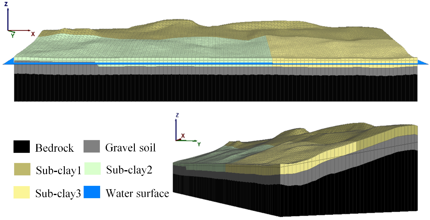
Based on the geological investigation data and the topographic data for sections K195+460 to K195+950, a numerical mesh model was developed (Figure 2). The bottom elevation of the model was 100.0 m and the maximum difference in slope elevation was 59.2 m, with the highest elevation being 210.6 m. The lengths in the X and Y directions were 490.0 m and 171.0 m, respectively, and the element type was wedge-shaped, with dimensions between 4.0 m and 5.0 m. The Mohr–Coulomb model was adopted, and the physicomechanical values from laboratory experiments and previous studies are summarized in Table 1 [31,32]. For the numerical analysis, the bottom of the model was fixed-boundary constrained and the top surface was unconstrained. The phased elasto-plastic solution method was employed to calculate the initial ground stress.
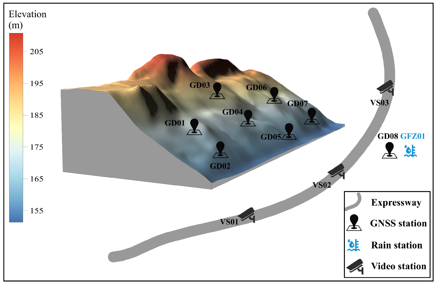
In November 2018, in the field investigation, prominent deformation characteristics were still found on this slope: wall cracking, gutter deformation, hill collapse, etc. (Figure 3). Considering the safety of the residents and the normal operation of the highway, a GNSS online monitoring system was constructed and started to operate in April 2019 [37]. The monitoring contents include the ground displacement, rainfall, and site environment, and the locations of the monitoring stations are shown in Figure 4. Stations GD01–GD07 are designed to monitor the ground displacement, and GD08 is located on the roof of the civil building opposite the slope as a relatively stable reference station. The GNSS results are obtained using relative static positioning with a 1 h solution strategy [38]. A GFZ-01 digital rain gauge is located at the same location as GD08. Three cameras are placed along the road to monitor the safety of the landslide and the road. The contents and methods of the monitoring system are described in Table 2.

2.3. GWR for Slope Physical Modelling

GWR is an extension of the conventional least-squares regression method. It assumes that the regression coefficients are multidimensional functions of the geographic location. GWR is an important tool for modelling the heterogeneity of spatial relationships [39,40]. In slope physical modelling, slopes have complex topographic and geological features, and their deformations show notable spatial heterogeneity. To establish a functional relationship between the physicomechanical parameters of a slope and its displacement, it should be assumed that the regression coefficients are three-dimensional functions of the spatial location. Let Y i be the displacement of i monitoring stations and X the physicomechanical parameters of the formation. The GWR function model used for slope physical modelling can be rewritten as follows [41]:
Y i = β 0 x i , y i , z i + k = 1 d β k x i , y i , z i X i k + ε i   ,     i = 1 , 2 , , n     k = 1 , 2 , , d
where Y i and X i k are the dependent and independent variables, respectively; x i , y i , z i are the spatial location coordinates of a point; β k ( x i , y i , z i ) is a function of the kth regression coefficient; and β 0 x i , y i , z i   and ε i are the constant and error terms of the regression model, respectively. In the GWR model, each coefficient β k ( x , y , z ) has a continuous second-order partial derivative for the spatial location coordinate. Given a spatial location ( x m , y m , z m ) , and according to the Taylor expansion of the multivariate function, the coefficients can be approximated as:
β k ( x , y , z ) β k ( x m , y m , z m ) + β k ( x ) ( x m , y m , z m ) ( x x m )                               + β k ( y ) ( x m , y m , z m ) ( y y m ) + β k ( z ) ( x m , y m , z m ) ( z z m )
where β k ( x ) ( x m , y m , z m ) , β k ( y ) ( x m , y m , z m ) , and β k ( z ) ( x m , y m , z m ) are the partial derivatives of β k ( x , y , z ) with respect to x , y , z at ( x m , y m , z m ) , respectively. According to the least-squares principle, the least-squares objective function constructed for any point ( x m , y m , z m ) is:
f ( β ( x m , y m , z m ) ) = i = 1 n { Y i k = 0 d [ β k ( x m , y m , z m ) + β k ( x ) ( x m , y m , z m ) ( x x m )                               + β k ( y ) ( x m , y m , z m ) ( y y m ) + β k ( z ) ( x m , y m , z m ) ( z z m ) ] X i k } 2 w i ( x m , y m , z m )
For this weighted least-squares problem, the solutions for the regression coefficients can be expressed with matrix notation. Let I d + 1 , 0 d + 1 be a unit matrix of order d + 1 and a zero-square matrix, respectively, and let X ( x m , y m , z m ) = [ X 1 ( x m , y m , z m ) , X 2 ( x m , y m , z m ) ] .
X 1 ( x m , y m , z m ) = 1 X 11 X 1 d     x 1 x m ( x 1 x m ) X 11 ( x 1 x m ) X 1 d 1 X 21 X 2 d     x 2 x m ( x 2 x m ) X 21 ( x 2 x m ) X 2 d                                                                                                                   1 X n 1 X n d     x n x m ( x n x m ) X n 1 ( x n x m ) X n d
X 2 ( x m , y m , z m ) = y 1 y m     ( y 1 y m ) X 11 ( y 1 y m ) X 1 d     z 1 z m ( z 1 z m ) X 11 ( z n z m ) X 1 d y 2 y m     ( y 2 y m ) X 21 ( y 2 y m ) X 2 d     z 2 z m ( z 2 z m ) X 21 ( z n z m ) X 2 d                                                                                                                                                                                         y n y m ( y n y m ) X n 1 ( y n y m ) X n d z n z m ( z n z m ) X n 1 ( z n z m ) X n d
By taking the partial derivative of Equation (3) with respect to β k ( u m , v m , t m ) ( k = 0 , 1 , , d ) and setting it as equal to 0, an estimate of the regression coefficient can be obtained:
β ^ ( x m , y m , z m ) = ( β ^ 0 ( x m , y m , z m ) , , β ^ d ( x m , y m , z m ) ) T                     = ( I d + 1 , 0 d + 1 , 0 d + 1 , 0 d + 1 ) [ X T ( x m , y m , z m ) W ( x m , y m , z m )                     X ( x m , y m , z m ) ] 1 X T ( x m , y m , z m ) W ( x m , y m , z m ) Y
where W ( x m , y m , z m ) = diag ( w 1 , w 2 , , w n ) is the spatial-weights matrix; its computation is described in Section 2. The estimated values of the regression coefficients for each sampling point can be obtained by taking ( x m , y m , z m ) = ( x i , y i , z i ) ( i = 1 , 2 , , n ) .
β ^ ( x i , y i , z i ) = ( β ^ 0 ( x i , y i , z i ) , , β ^ d ( x i , y i , z i ) ) T
Then, the fitted value of the response quantity Y at the sampling point i can be calculated with the following equation:
Y ^ i = X i β ^ ( x i , y i , z i )               = X i ( I d + 1 , 0 d + 1 , 0 d + 1 , 0 d + 1 ) [ X T ( x i , y i , z i ) W ( x i , y i , z i )     X ( x i , y i , z i ) ] 1 X T ( x i , y i , z i ) W ( x i , y i , z i ) Y
where X i is the ith row of the matrix X . Generally, in practical applications, it is easier to perform programming and calculations by using the matrix representation of Equation (8):
  Y ^ = ( Y ^ 1 , Y ^ 2 , , Y ^ n ) T = L Y
L = ( X 1 T , 0 1 × 3 ( d + 1 ) ) [ X T ( x 1 , y 1 , z 1 ) W ( x 1 , y 1 , z 1 ) X ( x 1 , y 1 , z 1 ) ] 1 X T ( x 1 , y 1 , z 1 ) W ( x 1 , y 1 , z 1 ) ( X 2 T , 0 1 × 3 ( d + 1 ) ) [ X T ( x 2 , y 2 , z 2 ) W ( x 2 , y 2 , z 2 ) X ( x 2 , y 2 , z 2 ) ] 1 X T ( x 2 , y 2 , z 2 ) W ( x 2 , y 2 , z 2 ) ( X n T , 0 1 × 3 ( d + 1 ) ) [ X T ( x n , y n , z n ) W ( x n , y n , z n ) X ( x n , y n , z n ) ] 1 X T ( x n , y n , z n ) W ( x n , y n , z n )
Finally, based on the fitted and observed values, the residual sum of squares (RSS) of the model and its variance estimates can be obtained as follows:
σ ^ 2 = RSS tr ( ( I L ) T ( I L ) ) = Y ^ T ( I L ) T ( I L ) Y ^ tr ( ( I L ) T ( I L ) )

2.4. Displacement Back-Analysis Method Based on GWR

The traditional optimal back-analysis method calculates the objective function error value using Equation (12), and the equivalent physicomechanical parameters are obtained when the objective function is optimal [42]:
V Obj = i = 1 n p i v i 2 = i = 1 n p i S i ( X ) L i 2
where L = ( L 1 , L 2 , , L n ) T contains n mutually independent observations, p = d i a g ( p 1   p 2     p n ) is the corresponding weight matrix, S i ( X ) is the displacement calculated using numerical simulation, and V O b j is the objective function.
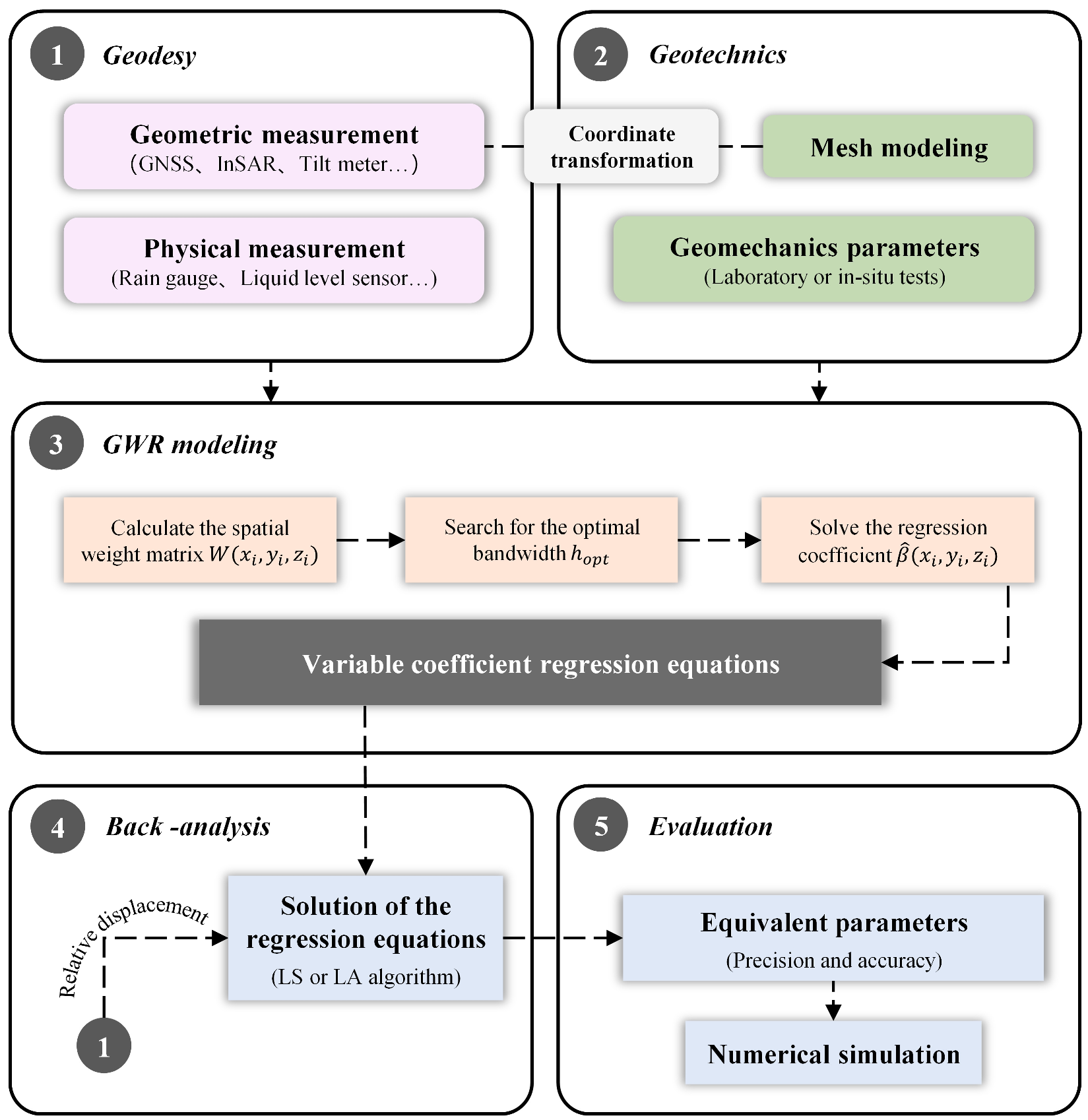
The intelligent optimal back-analysis method is an enhancement of the traditional method, but the essence of the algorithm is still based on minimizing the error between the observed and simulated displacements. When i > 1, there are i error values accumulated in the objective function. Then, there is a conflict problem within the multi-objective function; i.e., when the parameters are adjusted to optimize a certain error value, this results in the deterioration of other error values. In this situation, the solution to the multi-objective optimization problem is not unique [43,44]. To avoid this problem, as well as to describe the displacement back-analysis problem with analytical functions, a displacement back-analysis method based on GWR is proposed. First, GWR is employed to obtain the analytical equations for the displacement back-analysis problem. Then, by using the least-squares (LS) method and linear algebra (LA), the multi-objective displacement back-analysis is transformed into an analytical problem.
Before obtaining new observations, the stations recorded displacement data for a period of time. When the predisposing factors were known, the data for all stations during that period could be modelled with Equation (1) using GWR. The solution for the regression coefficient matrix from Equation (6) is critical, and the weights in the equation can be calculated using a bisquare kernel function or a Gaussian kernel function [41,45]:
w i ( m ) = 1 ( d i m / h ) 2 2 d i m h 0                                                     d i m > h
w i ( m ) = e x p ( ( d i m / h ) 2 )
where d i m is the distance from sampling point i to spatial point m , h is the bandwidth value, and the optimal bandwidth value h opt can be obtained by searching with the cross-validation (CV) method [46,47].
CV ( h ) = n ( n tr ( L ( h ) ) ) 2 i = 1 n Y i Y ^ i ( h ) 2 h opt = m i n h > 0 CV ( h )
where n is the number of spatial points; Y ^ i ( h ) and L ( h ) correspond to Equations (9) and (10), respectively; and h is the adopted bandwidth. After the optimal bandwidth is obtained, the regression coefficient matrix can be resolved, and the fitted values for each station and the residual sum of squares can be calculated according to Equations (9)–(11). The regression equations with variable coefficients are expressed below:
A n × ( d + 1 ) X ( d + 1 ) × 1 Y n × 1 = 0
where n and Y are the numbers of stations and their displacements, respectively, and d is the number of physicomechanical parameters. A is the coefficient matrix of the variable coefficient regression model, and the first column of the matrix is the constant term of the regression coefficient, so X = [ 1 X 1 X d ] T . Since the estimated parameter X contains the constant term of the regression coefficient, it is necessary to attach s constraints to X .
Φ s × 1   X = 0
If the physical triggering factors of the slope deformation can be measured, constraints can also be attached to them, such as the change in groundwater level. When newly observed displacements are available, Equations (16) and (17) can be solved. Generally, n + s d + 1 . When n + s = d + 1 and there is no conflict between the equations, the linear-algebra (LA) algorithm can be used to find the analytical solution to the equations. When n + s > d + 1 , the least-squares (LS) algorithm can be used to find the optimal solution to the overdetermined system of equations with X = ( A T A ) 1 A T Y . Here, the solution will be optimally unbiased.
The flowchart for the proposed DBA-GWR method is shown in Figure 5.

2.5. Instructions on Implementation of the Back-Analysis Method

Generally, the displacements calculated with numerical simulation represent the deformation generated by the whole process. Partial displacement usually occurs before the monitoring stations are deployed, which is called loss displacement, as shown in Figure 6. If the monitoring displacement, which is lower than the actual value, is considered the actual total displacement and compared with the simulated displacement, there will be inevitable bias. Although several approaches for calculating the loss displacement have been reported in the literature [48,49], on the whole, the loss displacement has an uncertain and empirical nature compared to the directly obtained monitoring displacement. Here, a new strategy is proposed. The relative displacement obtained from monitoring is used to fit the simulation results from a certain deformation process. Taking slope excavation as an example, excavation starts from the moment t 1 , and the displacement tends to stabilize by t 2 after the end of the excavation. The relative displacement S 12 obtained at moment t 1 t 2 can be used to fit the simulated displacement, and the equivalent physicomechanical slope parameters are easily obtained using the back-analysis method. In this study, relative displacement was used for modelling and back-analysis.
Coordinate conversion is an easily neglected aspect when implementing displacement back-analysis methods, especially in slope applications. Techniques such as real-time kinematic (RTK) positioning and unmanned aerial vehicle (UAV) photogrammetry are commonly used for slope topography measurements, and topographic data are used for mesh modelling [50]. Techniques such as the inclinometer, total-station, GNSS, and InSAR techniques are commonly used for slope ground and underground deformation measurement [51,52,53]. The measurement coordinate systems of the different techniques are distinct; in particular, the measurement system used with the inclinometer technique is a local coordinate system. When the coordinate system used for the displacement measurement is not consistent with the mesh model, there is systematic deviation between the simulated and measured displacements. Therefore, before implementing the displacement back-analysis method, appropriate means must be employed to render the coordinate systems of the mesh model consistent with those of the displacement measurements. The coordinate conversion method can be found in the literature [54,55,56].
The equivalent physicomechanical parameters determined with displacement back-analysis are generally verified by comparison with field measurements, including direct and indirect verification. Direct validation compares the equivalent parameters X ˜ d with the test results X d , and the relative error percentage (REP) can be used as the accuracy index of the parameters. Indirect validation compares the field monitoring results Y n of the monitoring stations with the simulation results Y ^ n by incorporating the equivalent parameters into the numerical model, and the root-mean-square error (RMSE) is often used as the accuracy index of displacement.
REP = X ˜ i X i / X i × 100 % RMSE = 1 n i = 1 n Y ^ i Y i 2

3. Results

3.1. Simulation Experiments

The proposed method was validated by using simulated data prior to the real-data experiments. The aim was to obtain an error-free slope dataset and to avoid the influence of coordinate-system bias on the back-analysis results.

3.1.1. GWR Modelling

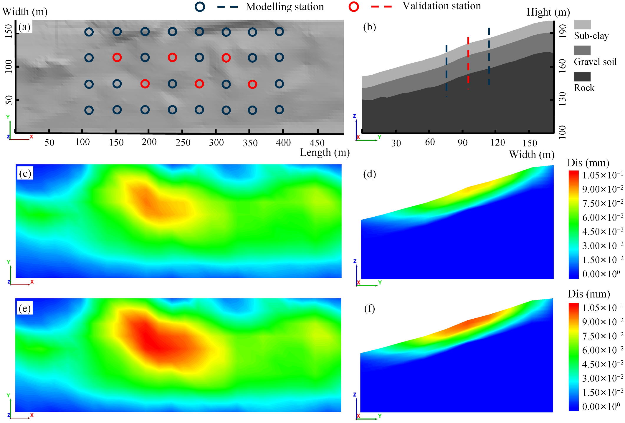
Thirty-two points were selected as ground displacement monitoring stations on the slope according to the principle of equal spacing: the data from 26 stations were used for GWR modelling and the remaining 6 stations were used for model validation (Figure 7a). Taking the mesh model at X = 254 m as a vertical section, three lines were selected as underground displacement monitoring stations, one of which was used for model validation (Figure 7b). By designing two scenarios (Table 3), two sets of slope displacement results, shown in Figure 7c–f, were obtained using simulation with FLAC3D software [57]. Finally, the data from the monitoring stations were exported to obtain a set of relative displacement data for GWR modelling and validation.
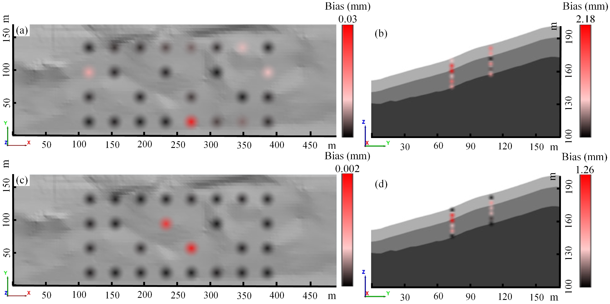
Six of the physicomechanical parameters and water-level-variation parameters shown in Table 3 were selected as the independent variables of the model. The displacements for the modelling stations in Figure 7a,b were used as response quantities for the GWR modelling. Two strategies were used to search for the optimal bandwidth. In strategy 1, the same bandwidth h was adopted for the ground stations and the underground stations. In strategy 2, different bandwidths were used for ground stations and underground stations: h 1 and h 2 , respectively. The model bandwidth was searched for using the CV criterion. The optimal bandwidth was h = 126   m for strategy 1 and h 1 = 105   m ,   h 2 = 21   m for strategy 2. The data were remodelled according to the obtained optimal bandwidth, and the model bias is shown in Figure 8. For the ground stations, the modelling performance with the two strategies was comparable. However, there were significant differences between the underground stations. The RMSE and the maximum bias of the model calculated with strategy 2 were 0.59 mm and 1.26 mm, respectively, which were better than those calculated with strategy 1, for which the RMSE and maximum bias were 1.24 mm and 2.18 mm, respectively. This indicates that using strategy 2 for bandwidth searching can result in GWR slope modelling with better fitting performance.

3.1.2. Back-Analysis Based on GWR

In the previous section, we demonstrated that it is feasible to establish an analytical function model of displacements and physicomechanical parameters using GWR. Therefore, when the relative displacement data from monitoring stations are available, the proposed DBA-GWR method can be employed to obtain the equivalent physicomechanical parameters for a period. To verify the feasibility of the method, four sets of slope relative-displacement data were obtained based on the parameters in Table 4 and applied for the back-analysis. The popular DBA-BPNN [31] method was employed using the displacement and target parameters as input and output layers, and the learning model was trained with the strategy of minimizing the target parameter error. This model enables high-accuracy predictions and, hence, this method was used for comparison. Unlike the proposed method, DBA-BPNN is an implicit function model. The training data for machine learning were obtained using the orthogonal test method.
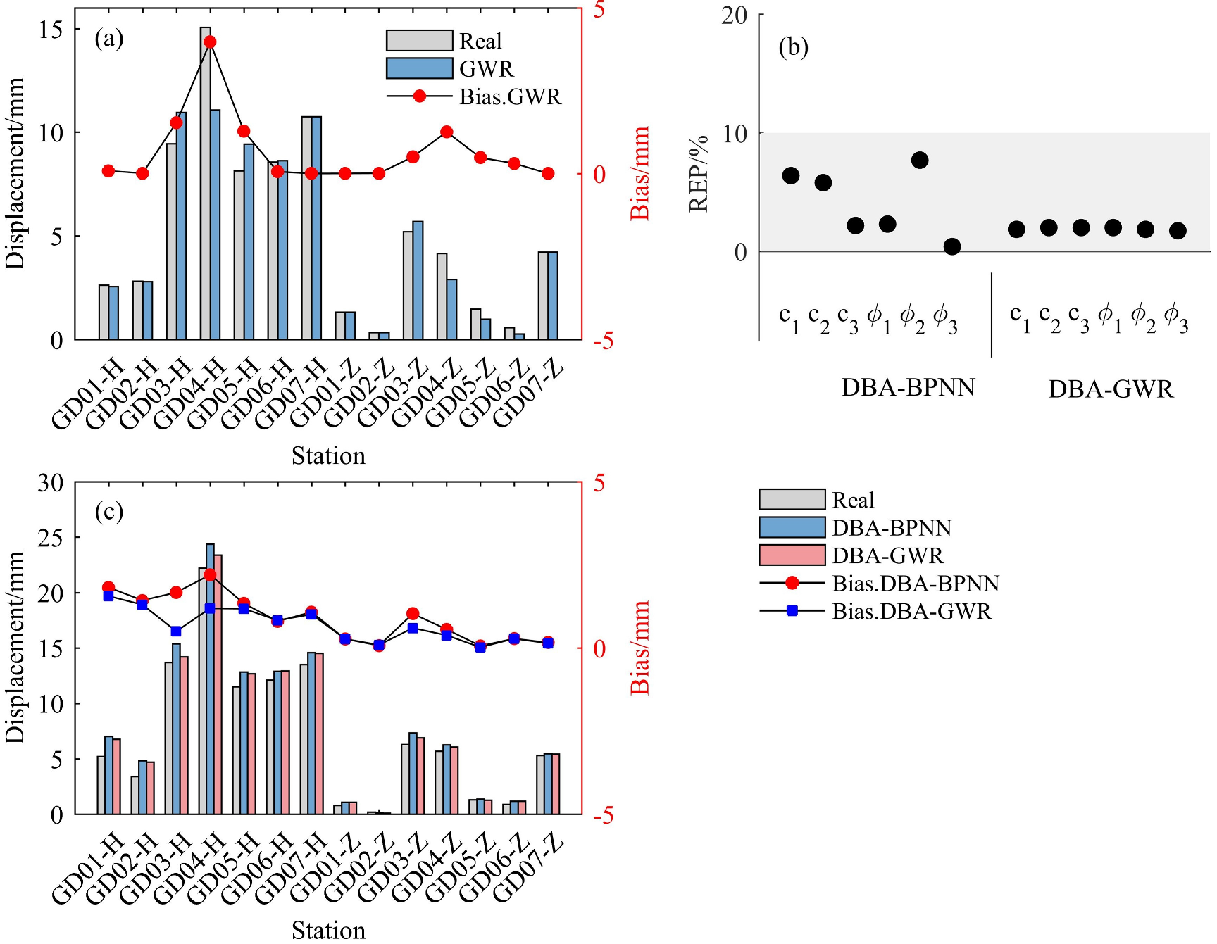
The accuracy of the inversion results for the four sets was counted with the REP, and an REP lower than 10% was used as the parameter tolerance interval for evaluation. As shown in Figure 9, the inversion results obtained with DBA-BPNN were correct for the data in sets 1 and 2. However, the data in sets 3 and 4 showed unsatisfactory performance, with some parameters located outside the interval. The accuracy rate of DBA-BPNN was only 75% (the accuracy rate was equal to the number of REPs lower than 10% divided by the number of equivalent parameters). Compared to the DBA-BPNN method, the DBA-GWR method achieved a higher accuracy rate of 100%, and the obtained parameters all lay within the interval. After that, the equivalent parameters determined with the DBA-GWR method were used in the forward calculation, and the simulated displacements for the validation stations were obtained. After statistical analysis, the precision with the first sets of data was lower than that with the other sets, but the RMSE and maximum bias were only 3.3 mm and 4.8 mm, respectively. This indicates that the proposed method could not only obtain more accurate equivalent parameters but also had good displacement precision.
Through the above simulation data experiments, we verified the feasibility of using GWR for slope physical modelling and parameter inversion. For the equivalent physicomechanical parameter inversion, in addition to the improvement in the accuracy rate, it was more meaningful that the proposed method could obtain the analytical expressions for the displacement back-analysis problem. In particular, the inversion results for the least-squares estimation were optimally unbiased.

3.2. Real Data Experiments

3.2.1. Monitoring Data

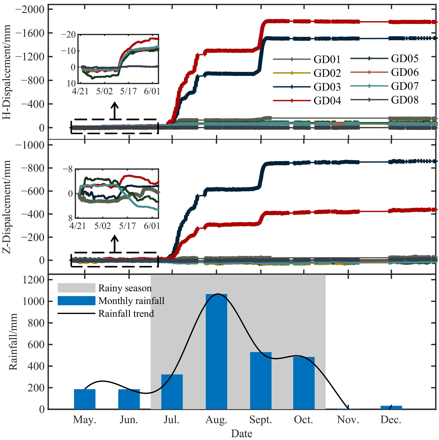
The online monitoring system recorded the development of the slope deformation from April 2019 to the end of 2019. Figure 10 shows the cumulative deformation time-series curve and the monthly rainfall time-curve for the slope (the horizontal displacement is mainly in the y direction, and the x direction is negligible). It should be noted that, before establishing the mesh model, we rotated the digital elevation model (DEM) to make the slope direction correspond to the y direction of the coordinate system. Second, we performed coordinate conversion of the monitoring data to make them consistent with the coordinate system of the mesh model. Figure 10 shows that the slope had three stages in 2019 consisting of slow deformation, evenly accelerated deformation, and variable accelerated deformation, with the largest deformation in the y direction. The displacements of the monitoring stations GD03 and GD04 were alarming, with a maximum deformation rate of 148.4 mm/d. The displacement of the relatively stable station GD08 was less than 10 mm, which indicates that the station is relatively stable and the GNSS monitoring results are reliable. Furthermore, the effect of intensive rainfall on the slope deformation rate was significant, indicating that rainfall is the main factor inducing the accelerated deformation of this slope.

3.2.2. Modelling and Back-Analysis

The GNSS data indicated that the slope experienced a small accelerated deformation in May, which levelled off at the end of the month. This section uses the relative displacement data from 4/21 to 5/20 for GWR modelling. It is well-known that, during periods of concentrated rainfall, the reduction of soil suction and the consequent loss of shear strength can trigger shallow landslides [58]. Therefore, the shear strength parameters of the sub-clay layer were considered as target parameters. The GNSS displacements recorded from 5/21 to 6/20 were used for the back-analysis. The physical modelling parameters and validation parameters for both periods were obtained with the long short-term memory network algorithm predictions [32] and are shown in Table 5.
In the GWR modelling process, we selected the bisquare kernel function and Gaussian kernel function to calculate the spatial weight matrix, and the optimal bandwidths calculated with the CV criterion were 190 m and 110 m. However, the modelling performances of the two kernel functions were comparable, and the RMSEs of the models were both 1.2 mm. The modelling results using the bisquare kernel function are shown in Figure 11a. The model-fitting results were in good agreement with the measured results, and the maximum bias was 3.9 mm, which indicated that the model had high precision.
Both the DBA-BPNN and the proposed DBA-GWR methods were employed for the back-analysis. In the GWR model, in addition to the three combinations of shear strength parameters, the independent variables contained a constant and a value for the water-level change. Therefore, two constraints were added, as in Equation (17). Figure 11b shows the accuracy of the inversion results, and the REP was lower than 10%, the error tolerance interval for the parameters. Both methods determined the equivalent physicomechanical parameters with a perfect accuracy rate, but the proposed method had a lower error and higher stability than DBA-BPNN. Based on the equivalent parameters determined by the two methods, the horizontal and vertical displacements of the seven GNSS monitoring stations were obtained through simulation, as shown in Figure 11c. It can be seen that the displacements calculated by the DBA-GWR method deviated less from the measured displacement data. The quantitative results show that the RMSEs of the DBA-BPNN and DBA-GWR methods were 1.1 mm and 0.8 mm, respectively. The horizontal displacement of the GD04 monitoring station was the largest, and the bias of the DBA-GWR method was only 1.2 mm. The above results demonstrate the effectiveness of the proposed method.

3.2.3. Stability Assessment

Throughout the GNSS time-series curves recorded in 2019 (Figure 10), the deformation development at GD03 and GD04 underwent three stages; namely, initial deformation, even deformation, and accelerated deformation. These two stations entered the variable accelerated deformation stage from the beginning of July, and the accumulated displacement increased rapidly, with maximum displacement rates of 119.6 mm/d and 148.4 mm/d. According to the theory of slope creep-slip damage [59], assuming that the slope is not disturbed by external factors, it can be considered that the slope of this section is damaged. However, rainfall is the dominant factor inducing accelerated deformation of the slope. Therefore, the stability of this slope cannot be simply assessed with the three-stage displacement law.
Numerical simulation techniques provide a powerful analytical means to gain insight into landslide damage mechanisms. This experiment combined the displacement back-analysis method, finite difference method, and strength reduction method to investigate the stability of the slope at the section where GD03 and GD04 are located. Since rainfall infiltration increases groundwater pressure, these increased pressures in turn induce slope movement. Therefore, the fluid–structure interaction model was used for the slope. The equivalent parameters obtained with the DBA-GWR method were used in the numerical model, and the safety factor of the slope was obtained using the tensile–shear strength reduction method (FOS = 1.84), which indicated that the slope was stable in late June. Figure 12a,b show the simulation results for the displacement in the critical state (FOS = 1). It can be seen that the slope deformation was larger in the horizontal direction, which is consistent with the GNSS monitoring results. Horizontally, GD03 and GD04 are located in the severely deformed area. On 24 July 2019, the field investigation results revealed significant cracks around station GD03, as shown in Figure 12c,d. Vertically, the displacement direction of the toe of the slope moved upwards through shear damage. This was consistent with the bulges found at the toe of the slope, as shown in Figure 12e,f, which were found on the lower slope. These results and phenomena confirm the accuracy of the numerical simulation and back-analysis results.
Figure 12a shows that the horizontal displacements of GD03 and GD04 in the critical state were 2.880 m and 4.291 m, respectively. These results comprise a set of displacement thresholds that can be used to determine whether the slope is likely to fail. Using numerical simulation to analyse the damage mechanism in slopes is of great significance for disaster warnings relating to unstable slopes.

4. Discussion

The proposed DBA-GWR method can provide analytical solutions for displacement back-analysis problems, significantly improving the interpretability of models. It is worth investigating whether the increase in interpretability influences the accuracy of a model. Machine-learning prediction models trained with minimal errors in the physicomechanical parameters can guarantee the accuracy of the equivalent parameters, which is why we employed DBA-BPNN as a benchmark method for comparison in our experiments. Here, we also employed the optimized back-analysis method for the inversion of the measured data, using a well-trained BPNN model instead of the forward calculation of the numerical simulation and the PSO algorithm as an optimization-seeking method. The precision of the displacement and the accuracy of the equivalent parameters for the three methods are statistically presented in Table 6. The accuracy rate was calculated with the same definition as in Section 3.1.2.
Compared with the DBA-BPNN method, the optimized back-analysis method had a higher displacement precision. However, the accuracy of the equivalent parameters was unsatisfactory. This is reasonable since the optimized back-analysis method is based on the optimization criterion of minimizing the displacement errors between simulated and measured values. The local optimum problem and initial value dependence problem affecting the optimal back-analysis method have been frequently discussed [29]. These problems represent the limitations of the objective function optimality algorithm. The objective function has a unique optimal solution only when it is proven to be concave or convex in the interval [33]. Nevertheless, this scheme is optimal for displacement fitting but not for equivalent parameters. In contrast, the DBA-BPNN method, the network model of which is trained with the criterion of minimizing the errors in the mechanical parameters, led to the prediction of equivalent parameters with higher accuracy (Table 6). The proposed DBA-GWR method performed better than the optimized back-analysis method and DBA-BPNN method. On the one hand, this was attributed to the high precision of the GWR model (i.e., variable coefficient regression equations), which could accurately express the functional relationship between the displacements and the target parameters. On the other hand, the DBA-GWR method employs the least-squares method to solve the equations, and the parameters obtained had optimal unbiased characteristics. From the viewpoint of parameter estimation, this is not available with other implicit function models.
In practical applications, observed data often exhibit non-stationarity in a temporal and spatial sense [60,61,62]. The GWR model employed in this paper was static. When the observed data have notable temporal non-stationarity, the results of GWR inversion may have a certain bias. As highlighted by studies such as those dealing with real estate modelling and traffic flow modelling, stationary GWR models are unlikely to be supported [46,63]. To date, most back-analysis models still belong to the category of static models. The observed data had dynamic temporal characteristics, and there is a lack of research on back-analysis using time-varying monitoring data. GTWR is a spatial and temporal dynamic modelling approach that takes into account both the temporal and spatial properties of data. It has been shown to perform satisfactorily in the fields of earth science, environmental science, and public health [64,65,66,67]. Therefore, GTWR can be considered for slope spatial and temporal dynamic modelling and back-analysis. Furthermore, Bayesian updating may be another choice that can take into account temporal issues in the back-analysis problem [68]. These would be interesting future projects for us.

5. Conclusions

Uncertainty in physicomechanical parameters has a significant impact on the design, construction, and stability assessment of unstable slopes. Displacement back-analysis appears to be an effective means for determining equivalent physicomechanical slope parameters.
In this study, a novel displacement back-analysis method based on geographically weighted regression was proposed. Furthermore, in the context of measurement data processing, coordinate transformation and equivalent parameter quality evaluation were added to the existing back-analysis framework. Simulation and real-data experiments were conducted, and it was found that the proposed DBA-GWR method could significantly improve the computational accuracy compared to the advanced methods. In addition, another superior aspect of DBA-GWR was the establishment of an analytical function model for the displacement back-analysis problem. With the support of the least-squares algorithm, the multi-objective displacement back-analysis was turned into a simple analytical problem, and the solution for the back-analysis was unique.
The context of this study is the rapid development of modern deformation monitoring technology and the gradual enrichment of monitoring content. Potential methods face the challenges of multi-objective optimization, error impact analysis, and the uniqueness of the solutions existing in geotechnical inversions. The method proposed here provides a potential tool.

Author Contributions

Methodology, W.D. and Y.D.; software, Y.D.; investigation, W.D.; writing—original draft preparation, Y.D.; writing—review and editing, W.D. and J.X.; visualization, Y.D.; supervision, J.X.; project administration, W.D.; funding acquisition, W.D. All authors have read and agreed to the published version of the manuscript.

Funding

This research was funded by the National Natural Science Foundation of China (No. 42174053) and the Natural Science Foundation of Hunan Province, China (Grant No. 2021JJ30805). The APC was funded by the National Natural Science Foundation of China.

Data Availability Statement

The data presented in this study are available on request from the corresponding author.

Acknowledgments

We gratefully thank the editor and anonymous reviewers for their constructive comments that helped improve the manuscript. In addition, the authors are also grateful to Guangyin Lu and Dongxin Bai for allowing the use of their study sites.

Conflicts of Interest

The authors declare no conflict of interest.

References

  1. Kocaman, S.; Gokceoglu, C. A CitSci app for landslide data collection. Landslides 2019, 16, 611–615. [Google Scholar] [CrossRef]
  2. Aaron, J.; Loew, S.; Forrer, M. Recharge response and kinematics of an unusual earthflow in Liechtenstein. Landslides 2021, 18, 2383–2401. [Google Scholar] [CrossRef]
  3. Peternel, T.; Janza, M.; Segina, E.; Bezak, N.; Macek, M. Recognition of Landslide Triggering Mechanisms and Dynamics Using GNSS, UAV Photogrammetry and In Situ Monitoring Data. Remote Sens. 2022, 14, 3277. [Google Scholar] [CrossRef]
  4. Vyazmensky, A.; Stead, D.; Elmo, D.; Moss, A. Numerical analysis of block caving-induced instability in large open pit slopes: A finite element/discrete element approach. Rock Mech. Rock Eng. 2010, 43, 21–39. [Google Scholar] [CrossRef]
  5. Yin, Y.; Sun, P.; Zhang, M.; Li, B. Mechanism on apparent dip sliding of oblique inclined bedding rockslide at Jiweishan, Chongqing, China. Landslides 2011, 8, 49–65. [Google Scholar] [CrossRef]
  6. Wang, H.; Zhang, B.; Mei, G.; Xu, N. A statistics-based discrete element modeling method coupled with the strength reduction method for the stability analysis of jointed rock slopes. Eng. Geol. 2020, 264, 14. [Google Scholar] [CrossRef]
  7. Zhang, Y.; Zhang, Z.; Xue, S.; Wang, R.; Xiao, M. Stability analysis of a typical landslide mass in the Three Gorges Reservoir under varying reservoir water levels. Environ. Earth Sci. 2020, 79, 14. [Google Scholar] [CrossRef]
  8. Guo, C.; Ma, G.; Xiao, H.; Zhou, W.; Chen, H.; Zhou, Z.; Cheng, X. Displacement back analysis of reservoir landslide based on multi-source monitoring data: A case study of the Cheyiping landslide in the Lancang River Basin, China. Remote Sens. 2022, 14, 2683. [Google Scholar] [CrossRef]
  9. Sun, G.; Zheng, H.; Huang, Y.; Li, C. Parameter inversion and deformation mechanism of Sanmendong landslide in the Three Gorges Reservoir region under the combined effect of reservoir water level fluctuation and rainfall. Eng. Geol. 2016, 205, 133–145. [Google Scholar] [CrossRef]
  10. Feng, X.; Zhao, H.; Li, S. A new displacement back analysis to identify mechanical geo-material parameters based on hybrid intelligent methodology. Int. J. Numer. Anal. Methods Geomech. 2004, 28, 1141–1165. [Google Scholar] [CrossRef]
  11. Miranda, T.; Dias, D.; Eclaircy-Caudron, S.; Correia, A.G.; Costa, L. Back analysis of geomechanical parameters by optimisation of a 3D model of an underground structure. Tunn. Undergr. Space Technol. 2011, 26, 659–673. [Google Scholar] [CrossRef]
  12. Li, S.; Zhao, H.; Ru, Z.; Sun, Q. Probabilistic back analysis based on Bayesian and multi-output support vector machine for a high cut rock slope. Eng. Geol. 2016, 203, 178–190. [Google Scholar] [CrossRef]
  13. Wu, C.; Hong, Y.; Chen, Q.; Karekal, S. A modified optimization algorithm for back analysis of properties for coupled stress-seepage field problems. Tunn. Undergr. Space Technol. 2019, 94, 7. [Google Scholar] [CrossRef]
  14. Zhao, H.; Yin, S. Geomechanical parameters identification by particle swarm optimization and support vector machine. Appl. Math. Model. 2009, 33, 3997–4012. [Google Scholar] [CrossRef]
  15. Zheng, D.; Cheng, L.; Bao, T.; Lv, B. Integrated parameter inversion analysis method of a CFRD based on multi-output support vector machines and the clonal selection algorithm. Comput. Geotech. 2013, 47, 68–77. [Google Scholar] [CrossRef]
  16. Zhao, H. A reduced order model based on machine learning for numerical analysis: An application to geomechanics. Eng. Appl. Artif. Intell. 2021, 100, 11. [Google Scholar] [CrossRef]
  17. Sun, P.; Bao, T.; Gu, C.; Jiang, M.; Wang, T.; Shi, Z. Parameter sensitivity and inversion analysis of a concrete faced rock-fill dam based on HS-BPNN algorithm. Sci. China-Technol. Sci. 2016, 59, 1442–1451. [Google Scholar] [CrossRef]
  18. Gao, W.; Ge, M. Back analysis of rock mass parameters and initial stress for the Longtan tunnel in China. Eng. Comput. 2016, 32, 497–515. [Google Scholar] [CrossRef]
  19. Qi, C.; Fourie, A. A real-time back-analysis technique to infer rheological parameters from field monitoring. Rock Mech. Rock Eng. 2018, 51, 3029–3043. [Google Scholar] [CrossRef]
  20. Li, H.; Wang, G.; Wei, B.; Zhong, Y.; Zhan, L. Dynamic inversion method for the material parameters of a high arch dam and its foundation. Appl. Math. Model. 2019, 71, 60–76. [Google Scholar] [CrossRef]
  21. Dong, K.; Yang, D.; Chen, J.; Zhou, J.; Li, J.; Lu, X.; Pei, L.; Kou, Q. Monitoring-data mechanism-driven dynamic evaluation method for slope safety. Comput. Geotech. 2022, 148, 9. [Google Scholar] [CrossRef]
  22. Qi, C.; Fourie, A.; Zhao, X. Back-analysis method for stope displacements using gradient-boosted regression tree and firefly algorithm. J. Comput. Civil. Eng. 2018, 32, 10. [Google Scholar] [CrossRef]
  23. Ghorbani, E.; Moosavi, M.; Hossaini, M.F.; Assary, M.; Golabchi, Y. Determination of initial stress state and rock mass deformation modulus at Lavarak HEPP by back analysis using ant colony optimization and multivariable regression analysis. Bull. Eng. Geol. Environ. 2021, 80, 429–442. [Google Scholar] [CrossRef]
  24. Yang, L.; Su, H.; Wen, Z. Improved PLS and PSO methods-based back analysis for elastic modulus of dam. Adv. Eng. Softw. 2019, 131, 205–216. [Google Scholar] [CrossRef]
  25. Zhang, Y.; Su, G.; Li, Y.; Wei, M.; Liu, B. Displacement back-analysis of rock mass parameters for underground caverns using a novel intelligent optimization method. Int. J. Geomech. 2020, 20, 15. [Google Scholar] [CrossRef]
  26. Sun, Y.; Jiang, Q.; Yin, T.; Zhou, C. A back-analysis method using an intelligent multi-objective optimization for predicting slope deformation induced by excavation. Eng. Geol. 2018, 239, 214–228. [Google Scholar] [CrossRef]
  27. Sun, Y.; Huang, J.; Jin, W.; Sloan, S.; Jiang, Q. Bayesian updating for progressive excavation of high rock slopes using multi-type monitoring data. Eng. Geol. 2019, 252, 1–13. [Google Scholar] [CrossRef]
  28. Zheng, Y.; Zhang, L.; Zhang, J.; Zheng, J.; Yu, Y. Multi-objective probabilistic inverse analysis of rainfall-induced landslide based on time-varied data. Rock Soil Mech. 2017, 38, 3371. [Google Scholar] [CrossRef]
  29. Li, Z.; Gong, W.; Zhang, L.; Wang, L. Multi-objective probabilistic back analysis for selecting the optimal updating strategy based on multi-source observations. Comput. Geotech. 2022, 151, 15. [Google Scholar] [CrossRef]
  30. Li, J.; Wu, Z.; Chen, J. An advanced Bayesian parameter estimation methodology for concrete dams combining an improved extraction technique of hydrostatic component and hybrid response surface method. Eng. Struct. 2022, 267, 16. [Google Scholar] [CrossRef]
  31. Xing, H.; Zhang, H.; Liu, L.; Yao, D. Comprehensive monitoring of talus slope deformation and displacement back analysis of mechanical parameters based on back-propagation neural network. Landslides 2021, 18, 1889–1907. [Google Scholar] [CrossRef]
  32. Dai, Y.; Dai, W.; Yu, W.; Bai, D. Determination of landslide displacement warning thresholds by applying DBA-LSTM and numerical simulation algorithms. Appl. Sci. 2022, 12, 6690. [Google Scholar] [CrossRef]
  33. Huang, Y. Study of uniqueness of multi-parameter inverse analysis of elastic displacement of concrete gravity dam. Eng. Optimiz. 2020, 52, 2033–2043. [Google Scholar] [CrossRef]
  34. Kupfer, J.; Farris, C. Incorporating spatial non-stationarity of regression coefficients into predictive vegetation models. Landsc. Ecol. 2007, 22, 837–852. [Google Scholar] [CrossRef]
  35. Weissmann, G.S.; Fogg, G.E. Multi-scale alluvial fan heterogeneity modeled with transition probability geostatistics in a sequence stratigraphic framework. J. Hydrol. 1999, 226, 48–65. [Google Scholar] [CrossRef]
  36. Makaske, B. Anastomosing rivers: A review of their classification, origin and sedimentary products. Earth-Sci. Rev. 2001, 53, 149–196. [Google Scholar] [CrossRef]
  37. Bai, D.; Tang, J.; Lu, G.; Zhu, Z.; Liu, T.; Fang, J. The design and application of landslide monitoring and early warning system based on microservice architecture. Geomat. Nat. Hazards Risk 2020, 11, 928–948. [Google Scholar] [CrossRef]
  38. Wang, J.; Satirapod, C.; Rizos, C. Stochastic assessment of GPS carrier phase measurements for precise static relative positioning. J. Geod. 2002, 76, 95–104. [Google Scholar] [CrossRef]
  39. Fotheringham, A.S.; Brunsdon, C. Local forms of spatial analysis. Geogr. Anal. 1999, 31, 340–358. [Google Scholar] [CrossRef]
  40. Zhao, C.; Jensen, J.; Weng, Q.; Weaver, R. A geographically weighted regression analysis of the underlying factors related to the surface urban heat island phenomenon. Remote Sens. 2018, 10, 1428. [Google Scholar] [CrossRef] [Green Version]
  41. Wang, N.; Mei, C.; Yan, X. Local linear estimation of spatially varying coefficient models: An improvement on the geographically weighted regression technique. Environ. Plan. A 2008, 40, 986–1005. [Google Scholar] [CrossRef]
  42. Gioda, G.; Locatelli, L. Back analysis of the measurements performed during the excavation of a shallow tunnel in sand. Int. J. Numer. Anal. Methods Geomech. 1999, 23, 1407–1425. [Google Scholar] [CrossRef]
  43. Palancz, B.; Awange, J.L. Application of Pareto optimality to linear models with errors-in-all-variables. J. Geod. 2012, 86, 531–545. [Google Scholar] [CrossRef]
  44. Mirjalili, S.Z.; Mirjalili, S.; Saremi, S.; Faris, H.; Aljarah, I. Grasshopper optimization algorithm for multi-objective optimization problems. Appl. Intell. 2018, 48, 805–820. [Google Scholar] [CrossRef]
  45. Fotheringham, A.S.; Oshan, T.M. Geographically weighted regression and multicollinearity: Dispelling the myth. J. Geogr. Syst. 2016, 18, 303–329. [Google Scholar] [CrossRef]
  46. Huang, B.; Wu, B.; Barry, M. Geographically and temporally weighted regression for modeling spatio-temporal variation in house prices. Int. J. Geogr. Inf. Sci. 2010, 24, 383–401. [Google Scholar] [CrossRef]
  47. Yang, Z.; Dai, W.; Yu, W.; Shi, Q.; Santerre, R. Mixed geographically and temporally weighted regression for spatio-temporal deformation modelling. Surv. Rev. 2022, 54, 290–300. [Google Scholar] [CrossRef]
  48. Zhang, Y.; Su, G.; Liu, B.; Li, T. A novel displacement back analysis method considering the displacement loss for underground rock mass engineering. Tunn. Undergr. Space Technol. 2020, 95, 15. [Google Scholar] [CrossRef]
  49. Zhao, Y.; Feng, S. Back analysis of surrounding rock parameters of tunnel considering displacement loss and space effect. Bull. Eng. Geol. Environ. 2021, 80, 5675–5692. [Google Scholar] [CrossRef]
  50. Jia, S.; Jin, A.; Zhao, Y. Application of UAV oblique photogrammetry in the field of geology survey at the high and steep slope. Rock Soil Mech. 2018, 39, 1130–1136. [Google Scholar] [CrossRef]
  51. Shamshiri, R.; Motagh, M.; Baes, M.; Sharifi, M.A. Deformation analysis of the Lake Urmia causeway (LUC) embankments in northwest Iran: Insights from multi-sensor interferometry synthetic aperture radar (InSAR) data and finite element modeling (FEM). J. Geod. 2014, 88, 1171–1185. [Google Scholar] [CrossRef]
  52. Bevilacqua, A.; Neri, A.; De Martino, P.; Isaia, R.; Novellino, A.; Tramparulo, F.D.; Vitale, S. Radial interpolation of GPS and leveling data of ground deformation in a resurgent caldera: Application to Campi Flegrei (Italy). J. Geod. 2020, 94, 27. [Google Scholar] [CrossRef] [Green Version]
  53. Chang, Z.; Wang, Y.; Qian, S.; Zhu, J.; Wang, W.; Liu, X.; Yu, J. An approach for retrieving complete three-dimensional ground displacement components from two parallel-track InSAR measurements. J. Geod. 2020, 94, 12. [Google Scholar] [CrossRef]
  54. Shen, Y.; Chen, Y.; Zheng, D. A quaternion-based geodetic datum transformation algorithm. J. Geod. 2006, 80, 233–239. [Google Scholar] [CrossRef]
  55. Li, B.; Shen, Y.; Li, W. The seamless model for three-dimensional datum transformation. Sci. China-Earth Sci. 2012, 55, 2099–2108. [Google Scholar] [CrossRef]
  56. Ge, Y.; Yuan, Y.; Jia, N. More efficient methods among commonly used robust estimation methods for GPS coordinate transformation. Surv. Rev. 2013, 45, 229–234. [Google Scholar] [CrossRef]
  57. Itasca, F. Fast Lagrangian Analysis of Continua; Itasca Consulting Group Inc.: Minneapolis, MN, USA, 2000. [Google Scholar]
  58. Pradhan, S.; Toll, D.G.; Rosser, N.J.; Brain, M.J. An investigation of the combined effect of rainfall and road cut on landsliding. Eng. Geol. 2022, 307, 16. [Google Scholar] [CrossRef]
  59. Xu, Q.; Yuan, Y.; Zeng, Y.; Hack, R. Some new pre-warning criteria for creep slope failure. Sci. China-Technol. Sci. 2011, 54, 210–220. [Google Scholar] [CrossRef]
  60. Darbeheshti, N.; Featherstone, W.E. Non-stationary covariance function modelling in 2D least-squares collocation. J. Geod. 2009, 83, 495–508. [Google Scholar] [CrossRef] [Green Version]
  61. Shi, Q.; Dai, W.; Santerre, R.; Li, Z.; Liu, N. Spatially heterogeneous land surface deformation data fusion method based on an enhanced spatio-temporal random effect model. Remote Sens. 2019, 11, 1084. [Google Scholar] [CrossRef] [Green Version]
  62. Yan, H.; Dai, W.; Xie, L.; Xu, W. Fusion of GNSS and InSAR time series using the improved STRE model: Applications to the San Francisco Bay Area and Southern California. J. Geod. 2022, 96, 20. [Google Scholar] [CrossRef]
  63. Ma, X.; Zhang, J.; Ding, C.; Wang, Y. A geographically and temporally weighted regression model to explore the spatiotemporal influence of built environment on transit ridership. Comput. Environ. Urban Syst. 2018, 70, 113–124. [Google Scholar] [CrossRef]
  64. Wang, H.; Zhang, B.; Liu, Y.; Liu, Y.; Xu, S.; Zhao, Y.; Chen, Y.; Hong, S. Urban expansion patterns and their driving forces based on the center of gravity-GTWR model: A case study of the Beijing-Tianjin-Hebei urban agglomeration. J. Geogr. Sci. 2020, 30, 297–318. [Google Scholar] [CrossRef]
  65. Ma, X.; Ji, Y.; Yuan, Y.; Van Oort, N.; Jin, Y.; Hoogendoorn, S. A comparison in travel patterns and determinants of user demand between docked and dockless bike-sharing systems using multi-sourced data. Transp. Res. Pt. A-Policy Pract. 2020, 139, 148–173. [Google Scholar] [CrossRef]
  66. Liu, J.; Li, S.; Ji, Q. Regional differences and driving factors analysis of carbon emission intensity from transport sector in China. Energy 2021, 224, 14. [Google Scholar] [CrossRef]
  67. Guo, B.; Wang, X.; Pei, L.; Su, Y.; Zhang, D.; Wang, Y. Identifying the spatiotemporal dynamic of PM2.5 concentrations at multiple scales using geographically and temporally weighted regression model across China during 2015–2018. Sci. Total Environ. 2021, 751, 15. [Google Scholar] [CrossRef] [PubMed]
  68. Kelly, R.; Huang, J. Bayesian updating for one-dimensional consolidation measurements. Can. Geotech. J. 2015, 52, 1318–1330. [Google Scholar] [CrossRef] [Green Version]
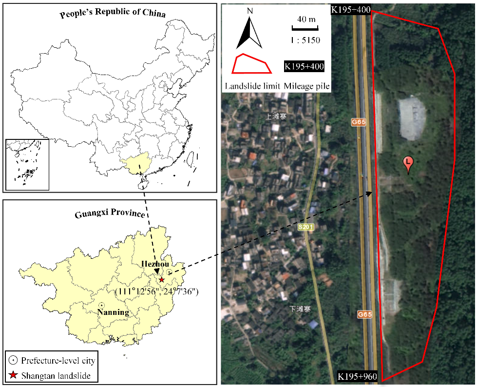
Figure 1. Location of the study site.
Remotesensing 15 00759 g001
Figure 2. The numerical mesh model of the study site.
Remotesensing 15 00759 g002
Figure 3. On-site findings in November 2018: (a) cracking of retaining wall, (b) guttering deformation, and (c) collapse.
Remotesensing 15 00759 g003
Figure 4. Location of the monitoring stations.
Remotesensing 15 00759 g004
Figure 5. Flowchart for the proposed DBA-GWR method.
Remotesensing 15 00759 g005
Figure 6. Monitoring displacement and loss displacement.
Remotesensing 15 00759 g006
Figure 7. Simulation datasets for the slope: (a,b) the setting of ground and underground displacement monitoring stations; the simulation results for the surface and profile, respectively, corresponding to (c,d) situation 1 and (e,f) situation 2. The length, width, and height in (a,b) correspond to the dimensions of the numerical model. (cf) share the same colour bar.
Remotesensing 15 00759 g007
Figure 8. The bias in the GWR model: deviations for the ground and underground stations, respectively, corresponding to strategy 1 (a,b) and (c,d) strategy 2.
Remotesensing 15 00759 g008
Figure 9. Accuracy of every inversion parameter.
Remotesensing 15 00759 g009
Figure 10. Data recorded by the monitoring system. In each direction, a partial zoom was produced for the pre-June data.
Remotesensing 15 00759 g010
Figure 11. (a) Comparison between the fitted values from the GWR and the measured values, (b) accuracy of the back-analysis results for different methods, and (c) comparison of the simulated and measured results.
Remotesensing 15 00759 g011
Figure 12. Simulation results and on-site findings: (a,b) displacement contours in the horizontal and vertical directions, respectively; (c,d) cracks around GD03; (e,f) bulges in the lower slope.
Remotesensing 15 00759 g012
Table 1. Summary of the main characteristics of the materials.
ParameterSymbolUnitySub-Clay 1–3Gravel SoilRock
Dry volumetric weight ρ kg × m - 3 220022002900
Bulk modulus K kPa 20601300
Shear modulus G MPa 1336800
Cohesion c kPa 10–161848
Angle of friction ϕ ° 10–14.51640,000
Biot modulus E MPa 4001000-
Infiltration coefficient n % 5050-
Table 2. Monitoring system contents and methods.
No.ContentMethodMonitoring InstrumentMonitoring Interval
1DisplacementGNSSHuace H3 GNSS Receiver1 h
2RainfallRain gaugeGFZ01 digital rain gauge20 min
3EnvironmentVideoHikvision surveillance cameraReal time
Table 3. Parameter settings for different situations.
PlanCohesion (kPa)Angle of Friction (°)Water (m)
c 1 c 2 c 3 ϕ 1 ϕ 2 ϕ 3
Initial1314.51716.51314A face
Situation 11213.5161612.2513↑0.5
Situation 21112.51515.511.512↑0.5
* Where “a face” refers to the water surface in Figure 2, and ↑ indicates rising water levels.
Table 4. Four sets of parameters for simulating the slope deformation.
SetsCohesion (kPa)Angle of Friction (°)Water (m)
c 1 c 2 c 3 ϕ 1 ϕ 2 ϕ 3
11011.5141510.7511↑0.5
29.51113.514.510.2510.5↑0.5
3910.513149.7510↑0.5
48.51012.513.59.259.5↑0.5
Table 5. Modelling parameters and validation parameters for different stages.
TimeCohesion (kPa)Angle of Friction (°)Water (m)
c 1 c 2 c 3 ϕ 1 ϕ 2 ϕ 3
Original data161516151517A face
5/2115.114.114.114.015.316.2↑0.4
6/2114.213.213.213.114.215.2↑0.9
Table 6. Precision and accuracy of equivalent parameters obtained with different methods.
MethodPrecision (mm)Accuracy
RMSEBias (max)Accuracy RateREP (max)
Optimal back-analysis0.92.383.3%10.2%
DBA-BPNN1.12.2100.0%7.7%
DBA-GWR0.81.6100.0%2.0%
Disclaimer/Publisher’s Note: The statements, opinions and data contained in all publications are solely those of the individual author(s) and contributor(s) and not of MDPI and/or the editor(s). MDPI and/or the editor(s) disclaim responsibility for any injury to people or property resulting from any ideas, methods, instructions or products referred to in the content.