Technical Note

Machine Learning of Usable Area of Gable-Roof Residential Buildings Based on Topographic Data

1
Faculty of Civil Engineering, Environmental and Geodetic Sciences, Technical University of Koszalin, Śniadeckich 2, 75-453 Koszalin, Poland
2
Faculty of Physics, University of Warsaw, Pasteura 5, 02-093 Warsaw, Poland
3
Department of Environmental Engineering and Geodesy, The Faculty of Production Engineering, University of Life Sciences in Lublin, Akademicka 13, 20-950 Lublin, Poland
*
Author to whom correspondence should be addressed.
Remote Sens. 2023, 15(3), 863; https://doi.org/10.3390/rs15030863
Submission received: 5 January 2023 / Revised: 31 January 2023 / Accepted: 1 February 2023 / Published: 3 February 2023
(This article belongs to the Special Issue Remote Sensing Image Processing in Poland)

Abstract

:
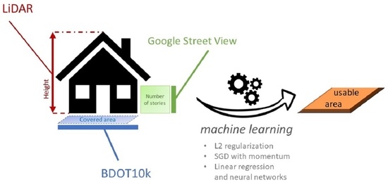
In real estate appraisal, especially of residential buildings, one of the primary evaluation parameters is the property’s usable area. When determining the property price, Polish appraisers use data from comparable transactions included in the Real Estate Price Register (REPR), which is highly incomplete, especially regarding properties’ usable areas. This incompleteness renders the identification of comparable transactions challenging and may lead to incorrect prediction of the property price. We address this challenge by applying machine learning methods to estimate the usable area of buildings with gable roofs based only on their topographic data, which is widely available in Poland in the Database of Topographic Objects (BDOT10k) of Light Detection and Ranging (LiDAR) origin. We show that three features are enough to make accurate predictions of the usable area: the covered area, the building’s height, and the number of stories optionally. A neural network trained on buildings from architectural bureaus reached a 4% median percentage error on the same source and 15% on the real buildings from the city of Koszalin, Poland. Therefore, the proposed method can be applied by appraisers to estimate the usable area of buildings with known transaction prices and solve the problem of finding comparable properties for appraisal.

Graphical Abstract

1. Introduction

The most reliable real estate appraisal technique is the so-called comparative approach [1,2]. In this approach, the appraiser compares the property in question to similar buildings that were sold recently on the market to evaluate the property’s price. One of the primary evaluation parameters for such comparisons is the usable area [3,4]. It is an especially dominant feature when it comes to residential buildings. When searching for transactions involving comparable buildings, Polish appraisers use the Polish Real Estate Price Register (REPR). The REPR includes data on real estate prices given in notarial deeds and is also an element of the cadastre [5,6,7,8,9,10,11]. However, previous works [12,13,14] have shown that the REPR is incomplete, especially concerning usable areas of residential buildings. A thorough examination of the REPR and its data on 800 properties located in Koszalin and Kołobrzeg counties in Poland showed that the information on usable space is present only in 40% of the studied cases. With such a limited number of properties with known usable areas, finding comparable transactions is difficult, which often renders an assessment of a property’s worth with the comparative approach impossible.
On the other hand, there is another publicly available source of data on properties that covers the whole territory of Poland, namely the Database of Topographic Objects (BDOT10k) [15]. The BDOT10k is a database that includes information on spatial location and descriptive attributes of topographic objects, such as covered areas and heights of the buildings. The information contained within the dataset is based on data originating from airborne Light Detection and Ranging (LiDAR) scanning, provided by the Information System of the National Guards against Extraordinary Threats (ISOK) Program [16]. If this widely available information could be translated into a usable area, it would solve the problem of Polish real estate appraisers. We propose machine learning to estimate the usable area of residential buildings based on their available topographic data. Machine learning has been widely used in real estate valuation [17,18,19,20], but not so much in estimating other features of buildings apart from their prices. Dawid et al. [21] demonstrated that in detached houses with flat roofs, the usable area can be estimated quite precisely based on such topographic data using neural networks. Their research, conducted using 96 projects of residential buildings from the architectural bureaus and 29 properties existing in Koszalin, Poland, has shown that the usable area can be estimated with great accuracy in the case of flat-roof buildings. Simple buildings (without garages and extensions) can be evaluated with great precision (3–4%). To take more complex properties into account, a simple neural network was used there, with a mean error of around 3.5%. Finally, the neural network they trained on the building designs was tested on real buildings located in Koszalin. The median error they obtained was below 9%, granting a satisfactory precision for identifying comparable transactions in the REPR.
Both the work of Dawid et al. [21] and ours use two distinct datasets composed of building designs from architectural bureaus and existing buildings in Koszalin. There are two reasons for this choice. First, contrary to real building measurements, designs from architectural bureaus provide a full detailed description of the building’s interior. This allowed for testing various parameter combinations in search of the one resulting in the best prediction results. Second, real building data are inevitably subjected to some measurement errors, a flaw that pure designs do not have. Since the machine learning model can only be as good as the data we train it on, using an available source of data not subject to measurement error is a clear advantage in this matter.
Here, we extend the proposed machine-learning approach of usable area estimation to residential buildings with gable roofs. A different roof structure creates new challenges for estimation methods, particularly by introducing slants that impact the usable area of the highest floors. We discuss this impact in Section 3.1 in light of the different norms used in practice in Poland, which make gathering data even more challenging. Another issue is the accuracy of airborne laser scanning, which may play a role when measuring the heights of gable-roof buildings (in contrast to flat-roof buildings). We discuss this issue and estimate the worst possible error depending on the roof slope in Section 3.2. After highlighting the challenges that gable roofs introduce, we present the accuracy of linear regression and neural networks trained on the gable-roof building data from architectural bureaus and tested on the same type of data in Section 3.3. Finally, we present the accuracy of those methods on real buildings from Koszalin, Poland, in Section 3.4.

2. Materials and Methods

2.1. On Polish Norms for Usable Area Calculation

To highlight the legal complexity of real estate appraisal in Poland, we start by explaining Polish norms for usable area calculation. The problem of calculating usable area in Poland due to existing various norms has already been discussed in many publications [22,23,24,25,26,27,28]. Until 1999, the usable area was commonly calculated using the PN-B-02365:1970 standard [29]. Then PN-ISO 9836:1997 was introduced [30]. Between 1999 and 2012, both standards were in use, and after 2012, PN-ISO 9836:1997 became obligatory for newly built properties, and two additional principles were imposed [31]. It is worth mentioning that the Polish Committee of Standardization withdrew PN-B-02365:1970 and PN-ISO 9836:1997, and since 2015, the recommended norm has been PN-ISO 9836:2015-12 [32], which remains unused due to a lack of a legal amendment. Those changes pose additional difficulties in using the REPR as the contained usable area may have been calculated using an unknown norm. As a result, the definition of residential units and the method of estimating usable areas have changed. Those changes, as well as the basic differences among norms, are described in detail in Refs. [21,33].

2.2. The Recommended Polish Norm and Gable-Roof Buildings

Here, we focus on the elements important only for buildings with gable roofs. According to this new act, 100% of the area of rooms or their parts with a height equal to or higher than 2.20 m should be included in the calculation, 50% of the area with a height equal to or higher than 1.40 m and less than 2.20 m should be included, and finally, an area with a height less than 1.40 m should be completely omitted. An important consequence of this act is also ignoring partitioning walls completely, in contrast to previous standards. Furthermore, this rule waives the PN-B-02365:1970 norm.

2.3. Simulation of Knee Wall Height Impact on Usable Area

To calculate the dependence of the usable area of a building with a gable roof on the building’s and its knee wall’s height, we used the program AutoCAD Civil 2015 and modeled a representative gable-roof building project [34]. The sketch of the modeled building is presented in Figure 1, which also shows the knee wall (distance from the ceiling to the wall plate, marked as h) and the height of the building (marked as H). Figure 1 also displays the verging heights for three used norms described in the previous Section 2.1: 140, 190, and 220 cm. To calculate the usable area, according to the project, the following characteristics were used: area of staircase: 4.2 m 2 , width of the partitioning walls: 12 cm, lining of the walls: 5 cm, and the surface of the chimney was omitted.

2.4. Data on Gable-Roof Properties from Architectural Bureaus

Training machine learning models requires valid and reliable data. Thus, to train machine learning models for usable area estimation, we decided to use the information available online from the architectural bureaus Lipińscy [35] and Archon [36]. Within this dataset, we have access to all the designs and their interiors, and we can easier understand and prevent potential errors in the model. In this work, we focus on buildings without garages and boiler rooms because they contribute to the covered area but not to the usable area and, as such, make the usable area estimation task more demanding. Moreover, the inclusion of garages and boiler rooms in the estimation task is already exhaustively discussed in Ref. [21], and proposed solutions can be readily applied here as a different roof structure has no impact on garages or boiler rooms.
The data gathered from both architectural bureaus are from a total of 172 single-family residential buildings with gable roofs. The usable area was provided according to the PN-ISO 9836: 1997 standard. We constructed this dataset out of 95 original building designs without garages and 77 building designs that we modified and removed garages or extensions. The parameters of these 172 residential buildings are presented in Table 1.

2.5. Data on Gable-Roof Residential Buildings in Koszalin from Airborne Laser Scanning

The second dataset used within this work is composed of real residential buildings from Koszalin, Poland. These are the target buildings whose usable area Polish real estate appraisers need to identify for a successful application of the comparative approach—the most reliable appraisal technique so far. Therefore, the performance of our estimation approach on this dataset is a litmus test of the method’s applicability to such a class of data.
Information on the parameters of Polish residential buildings is available for appraisers in the REPR in the respective Polish local administrative unit or county office, but we already noted in Section 1 that this register is highly incomplete. Therefore, we need an additional source of data. In this work, we propose to use the BDOT10k database [15], which contains LiDAR information, originating from airborne laser scanning, provided by the Information System of the National Guards against Extraordinary Threats (ISOK) Program [16]. It covers the whole territory of Poland and includes information on spatial location and descriptive attributes of topographic objects. The database contains descriptions of different kinds of topographic objects ranging from roads and waterways to buildings, the last of which will be our only point of interest in this database for the purpose of this work. Building descriptions in the database contain features such as height, width, length, and perimeter. The LiDAR scanning was conducted at two levels of detail (LoD): LoD1 and LoD2. The LoD1 contains a square grid of measurement points with a density of 4 pts/m 2 , neglects roof geometry, and contains only bodies of buildings. The LoD2 is characterized by a rectangular grid of measurement points, with a grid density of 12 pts/ 2 , containing roof structures and simple additional building textures such as extensions or garages. Most of the Polish LiDAR surface data exhibit LoD2, but residential buildings analyzed within this paper and located in Koszalin exhibit LoD1. The BDOT10k is available within the Geoportal database [37] managed by the Head Office of Geodesy and Cartography. Information from the Geoportal for the city of Koszalin was downloaded in the CityGML 2.0 standard. The information was accessed using the QGIS program [38]. Google Street View was used when information on the number of stories was missing in the REPR.
Twenty-four residential buildings with gable roofs and with accessible essential data and usable areas measured using the PN-ISO 9836:1997 norm were selected for the final test of the proposed machine learning model. The data comes from the notices on the Koszalin residential buildings’ construction completion sent to the District Construction Supervision Inspector of Koszalin. Such documents and permit applications are required to start using buildings. While we motivate our study by the availability of LiDAR data across Poland, which provides various topographic information on buildings, our analysis of errors of LoD1 height measurements (in Section 2.6 and Section 3.2) indicates that this level of detail causes additional challenges as it gives an estimate for the median of the building’s height. Therefore, to avoid at this stage errors of LoD1 height measurements, the studied Koszalin buildings have a known height measured by surveyors. The properties were mostly localized in a region of the European Union Housing Complex (pol. Osiedle Unii Europejskiej) in Koszalin. The characteristics of the buildings are presented in Table 1. They were built between 2020 and 2022.

2.6. Monte Carlo Simulation

To estimate the error that airborne laser scanning can make when measuring the height of the gable-roof building, we conducted a simulation using the Monte Carlo method. Those errors depend on the standards used during scanning, which are described in more detail in the previous Section 2.5. In particular, the heights of LoD1 models (obtained at the density of 4 pts/m 2 ) are determined as a median of heights of LiDAR data points within a building frame provided by BDOT10k. The heights of gable-roof LoD2 models (obtained at the density of 12 pts/m 2 ) are the maximum heights measured within the building frame.
In our simulations, whenever we kept any of the dimensions fixed, we assumed width = 12.44 m, depth = 15.65 m, and height = 2 m. The width and depth are taken as the representative averages of analyzed Koszalin county residential buildings, as seen in Ref. [21]. Moreover, it is worth noting that the calculated height measurement errors presented further in Section 3.2 are expressed as a percentage of actual modeled height.
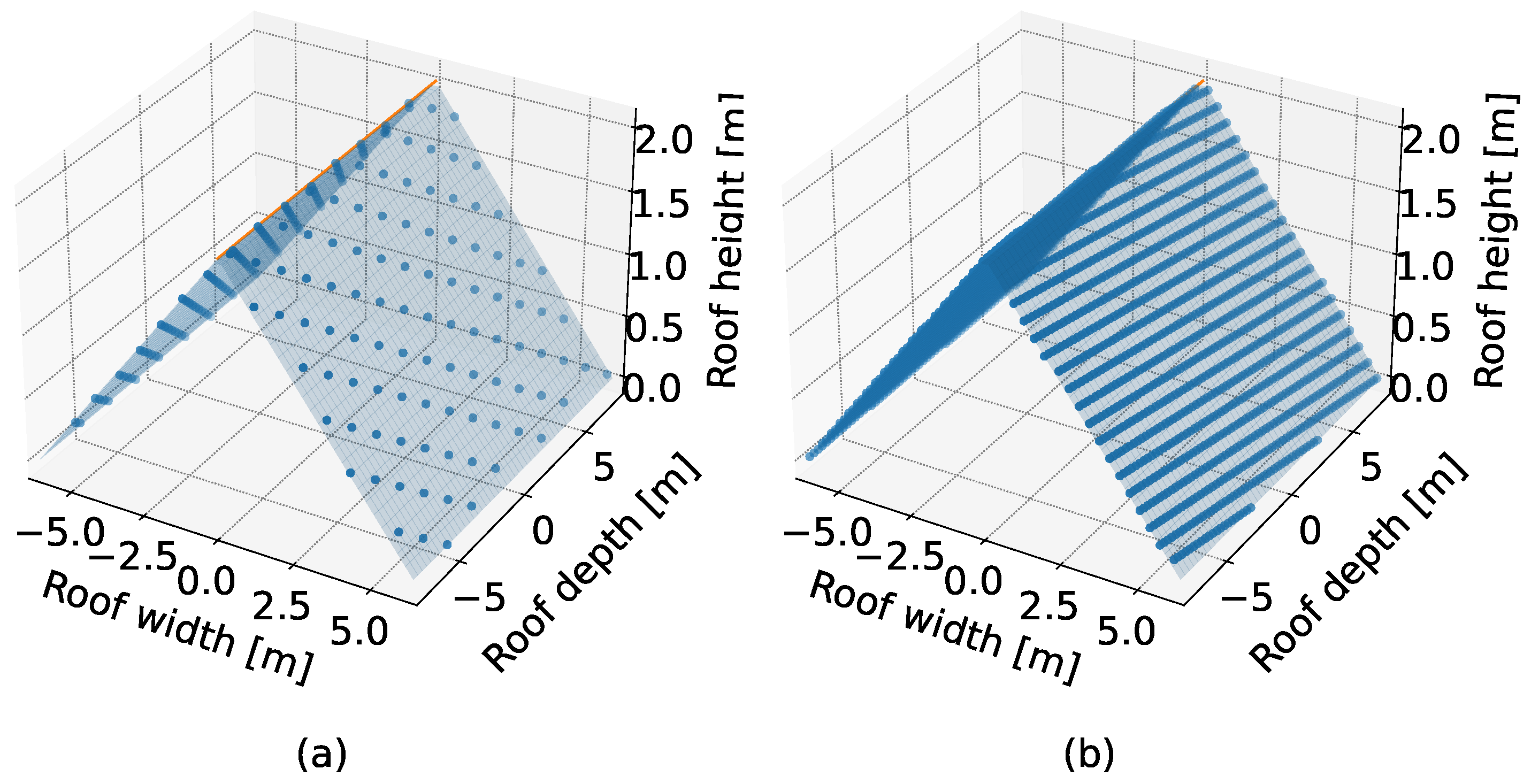
We calculated two types of errors: the worst-case-scenario measurement error (WCSME) and the mean measurement error (MME) for both LoD1 and LoD2 measurements. To do this, we first modeled a roof as a parametric surface z ( x ) = a · | x | + height , where a = height width / 2 . The LoD1 and LoD2 densities of 4 and 12 pts/m 2 , respectively, translate to measurement points distributed in a rectangular grid of 1 × 1 m spacing and 1 3 × 1 4 m spacing, as presented in Figure 2. For each configuration of roof dimensions (width, height, depth), we modeled the measurement errors for all possible scanning angles of an aircraft from range α [ 0 , π 2 ] , with 100 Monte Carlo steps for each angle, where by scanning angle we mean the angle in the X Y plane, between the measurement grid’s central axis and the line perpendicular to the roof ridge. This represents the possibility that the measurements grid is projected by an aircraft moving in a direction that is not co-linear with the roof ridge.
In a single Monte Carlo step, we conducted the following routine:
  • We sampled an initial point of the projected measurement grid from the uniform distribution. The point was sampled within a square of dimensions matching the grid’s spacing in the lower left corner of the roof;
  • Given this point, we constructed the measurement grid with the spacing representative of LoD1 or LoD2, which covered the whole roof, with 2 m padding on each side of the grid;
  • We then measured the height, matching the method to the given LoD:
    • For LoD1, the median value among the grid points is was what we modeled as the measured height;
    • For LoD2, the maximal value among grid points was what we modeled as the measured height.
After conducting 100 Monte Carlo steps for each angle for fixed roof dimensions, we computed each error as follows:
  • WCSME is the difference between the minimal measured height and the set height;
  • MME is the difference between the mean measured height (averaged across Monte Carlo steps for each angle and then averaged over all angles) from the set height.
Once defined, this routine was used to examine how the error changes upon varying roof width (for fixed height) or varying height (for fixed width).

2.7. Machine Learning Methods

A typical machine learning problem contains three vital parts: the dataset X, the model g ( θ ) , and the cost function we seek to minimize C ( X , g ( θ ) ) . The cost function is a measure of the model’s g ( θ ) performance on the dataset X at any given point in time, which is utilized to tune its parameters θ . This process of tuning the model’s parameters while minimizing the cost function is called training, or in the case of linear models, such as the regression, we also call it fitting. The changes in parameters are usually computed according to the Stochastic Gradient Descent (SGD) algorithm. In supervised learning problems (i.e., with data labels known as a priori), the heuristic is to divide the dataset into three mutually exclusive parts: training set, validation set, and test set. During the training process, the machine parameters θ are tuned in such a way that the loss computed on the training dataset is minimized with each iteration, i.e., training epoch. Additionally, we can tune the hyperparameters, i.e., learning rate, regularization strength, etc., to minimize the error on the validation dataset. After the training is completed, its results are assessed using the test dataset, which is a measure of how well the machine generalizes, that is, how well it performs on previously unseen data points. In our case, the dataset X is the data of the real estate characteristics such as the covered area, height, and the number of stories, along with their usable areas, i.e., labels.
The first machine learning model g ( θ ) we trained for this estimation task was the linear regression with bias. The loss function we minimized C ( X , g ( θ ) ) was the linear least squares function, with a penalization term added—L2 regularization. The need for the penalization term comes with the introduction of more features describing the buildings. As a result, our linear regression model became what is known in the literature as ridge regression, or Tikhonov regularization, with the aim of mitigating the problem of multicollinearity of the features. The L2 regularization we utilized also penalizes the increase of weights’ values and, as such, limits the tendency to focus on some features only.
The second machine learning models used within this work are neural networks with a single hidden layer with 10–30 hidden neurons. They were trained using stochastic gradient descent (SGD) with momentum and scheduled learning rate. All the hyperparameters can be found in the code in Ref. [39]. We mostly followed the machine learning approach described in Ref. [21].
For the purpose of both models’ training, validation, and testing, the architectural bureau designs dataset was split into three respective datasets: training, validation, and test dataset, with a split ratio of 60-20-20. Therefore, for a dataset consisting of 172 designs, this translates to train-val-test sizes of 104-34-34 data points of one- and two-story buildings. As we present the results in Section 3.3, these two building types are made distinguishable on the plots for the reader to be able to see the difference in the prediction performance.
In the following sections, we present the results of applying linear regression and simple neural networks to estimate the usable area of gable-roof residential buildings. In Section 3.3, we start with buildings from architectural bureaus [35,36] to have fully controllable training, validation, and test sets. When the usable area estimation is based solely on topographic data, with no access to interiors, we are unable to take into account any special interior designs, such as a mezzanine, that heavily impact the usable area, regardless of the complexity of the applied model. As we have access to all the designs and their interiors, we can understand potential errors in the model. On the contrary, if we trained the machine learning models on realistic buildings where we have no knowledge of interiors nor of the norm used to calculate its usable area, the model would be subjected to multiple sources of noise and imperfections that would deteriorate its accuracy. Therefore, we start here by training and testing the models on the controllable dataset, and then we test it on real buildings in Section 3.4.
There is various topographic information available within the BDOT10k [15] and LiDAR data accessible in Geoportal [37], the REPR, and Google Street View. We list them in Table 1: covered area in m 2 , height in m 2 , number of stories, and the height of the knee wall in m. Moreover, we can extract the building’s perimeter, width, and length. The first task is to find an optimal set of input features needed to estimate the usable area accurately. For the convenience of real estate appraisers, their number of input features should be minimal. This problem is discussed in Section 3.3.

3. Results

3.1. Gable Roofs Impact the Usable Area of the Building

Table 2 shows the impact of increasing the height of the knee wall of an exemplary building described in Section 2.3 on the usable area of its top floor, presented using three various norms. As discussed in Section 2.1, those norms are used in registers depending on the construction year of the building.
A higher knee wall decreases the roof slope, which changes the usable area. For example, increasing the knee wall from 14 to 25 cm increases the usable area of the top floor by 3.11, 4.44, and 3.20 m 2 within the PN 70, ISO 97, and ISO 2015, respectively. By increasing the knee wall’s height, the usable area converges to the case of a flat-roof building. From Table 2, we also see that differences between usable areas calculated using different norms can vary even by 10%.

3.2. Errors in the LiDAR-Based Data for Gable-Roof Buildings

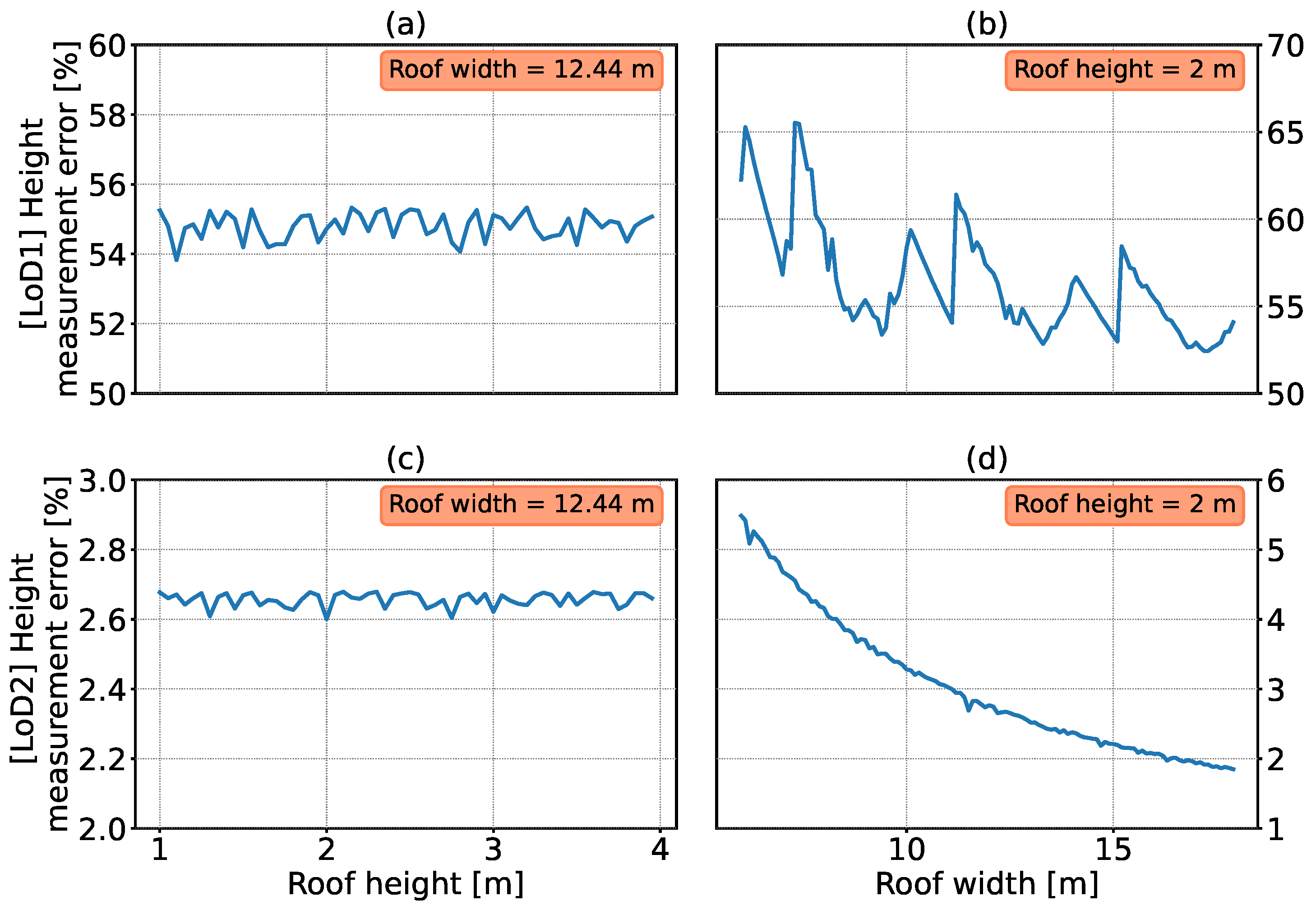
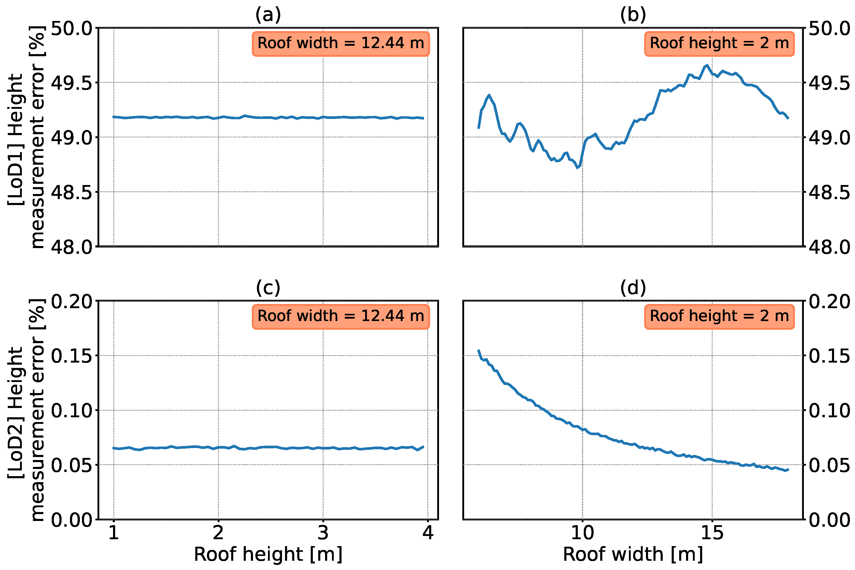
Gable roofs generate an additional challenge when relying on airborne laser scanning data to provide heights of the buildings. Intuitively, as you increase the slope of the roof and decrease the width, the worst-case scenario error that can be made during scanning should increase. In this section, we estimate the worst-case scenario (WCSME) and mean measurement (MME) errors, depending on the roof slope, in the case of LoD1 and LoD2 scanning data. We estimated them using the Monte Carlo technique with assumptions presented in Section 2.6. The dependence of the WCSME and MME on the roof width and height (so the roof slope) is presented in Figure 3 and Figure 4.
The WCSME for LoD1 is of the order of 55%, which is expected as the height is set in LoD1 as the median of height measurements. For a varying roof height in the range ( 0 , 4 ) m (with a roof width fixed at 12.44 m.), the WCSME oscillates around 55%. With an increasing roof width in the range ( 6 , 18 ) m (with a roof height fixed at 2 m), the WCSME decreases from 65 % to 50 %. The MME for LoD1 is around 50%. It oscillates around 49.2% and 49% when varying a roof height in the range ( 0 , 4 ) m (with a roof width fixed at 12.44 m) and when varying a roof width in the range ( 6 , 18 ) m (with a roof height fixed at 2 m), respectively. Interestingly, the mean error is mostly stable across these simulations and could be approximated by 50%.
The LoD2 errors are significantly smaller. Its WCSME is around 2.5%, and its MME is around 0.1%. The LoD2 MME decreases from 0.175 % to 0.05 % when a roof width increases in the range ( 6 , 18 ) m (with a roof height fixed at 2 m). When using buildings’ heights measured at LoD2, those errors can be safely ignored.

3.3. Machine Learning for Buildings of Architectural Bureaus

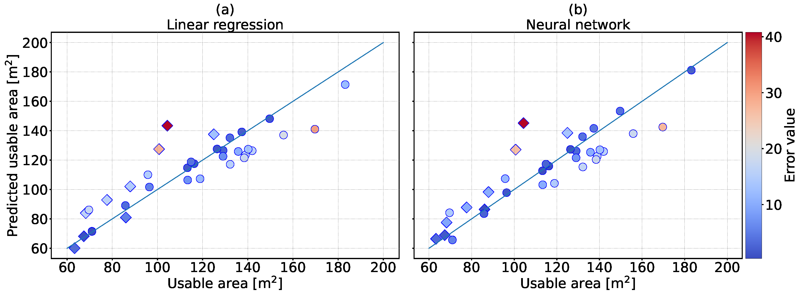
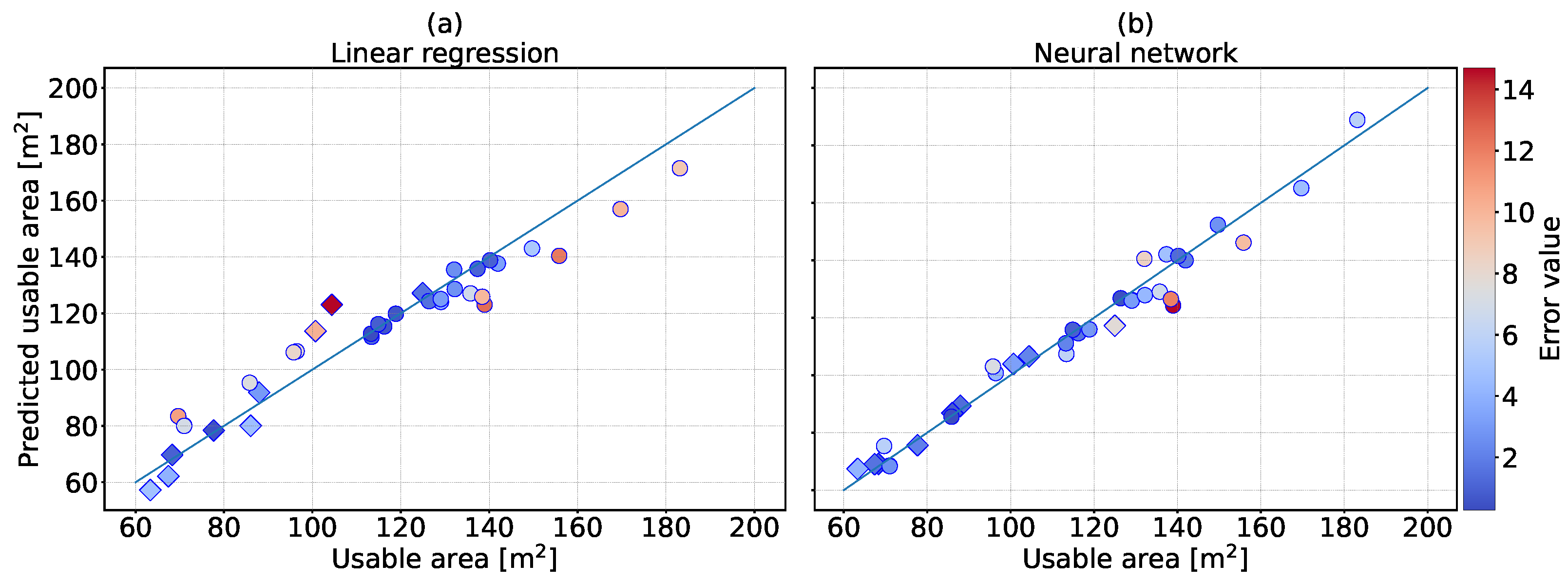
Firstly, we analyze the accuracy of the linear regression and neural network when estimating the usable area based only on the covered area and height of the building. We present the comparison of predicted and true usable areas in Figure 5 on the test set composed of 34 one- and two-story buildings from architectural bureaus. We also show the quality metrics such as R 2 , mean absolute error (MAE), median absolute error (MedAE), max and min error, and median absolute percentage error (MedAPE) in Table 3.
Let us analyze the test building that is the most confusing to both models (marked in red in Figure 5). This building design of Lipińsky called “Ostenda” is characterized by unusually high ceilings and has an attic. As a result, it is unusually high for a one-story building. When on average, one-story and two-story buildings in the dataset are 6.03 and 8.16 m high, respectively, this Ostenda building is 7.56 m high. With this example, we see that adding the number of stories as an input feature could improve the performance of both models as it helps by taking into account possible slants of the top floor or the attic.
Therefore, we analyze the accuracy of the linear regression and neural network when estimating the usable area based on the covered area, the height of the building, and the number of stories. We present the comparison of predicted and true usable areas in Figure 6 on the same test set. The performance metrics are also presented in Table 3. Finally, we see that both models reach a satisfying accuracy with R 2 around 95%, and MedAE around 5 m 2 . This time, the neural network performs significantly better than the linear regression. Having more tunable internal parameters than linear regression, the neural network can better model the dependence of the usable area on the two input features—the number of stories and the height. With the median absolute percentage error of 4%, the network successfully estimates the usable area of gable-roof buildings based only on their topographic data, i.e., the covered area, height of the building, and the number of stories.
Finally, we add more input features and check whether the model performance improves. After adding the knee wall’s height, the accuracy of both linear regression and neural network increases. They reach R 2 of 95% and 98% and MedAPE of 5% and 3%, respectively. However, the performance increase may not be worth the effort of extracting information on this input feature. An experienced real estate appraiser can use Google Street View to make an educated guess of the knee wall’s height, but this estimate is subjected to a significant error. Therefore, in the following section, we test the machine learning model without taking the knee wall’s height as an input feature.

3.4. Machine Learning for Real Buildings in Koszalin

As a final test of our approach, we apply the train neural network to estimate the usable area of the real 24 buildings in Koszalin, Poland. The information on these buildings comes from transactions, therefore we can rely on the reported height of the building, circumventing the problem of possible height measurement errors present in LoD1 LiDAR data, which we discussed in Section 3.2.
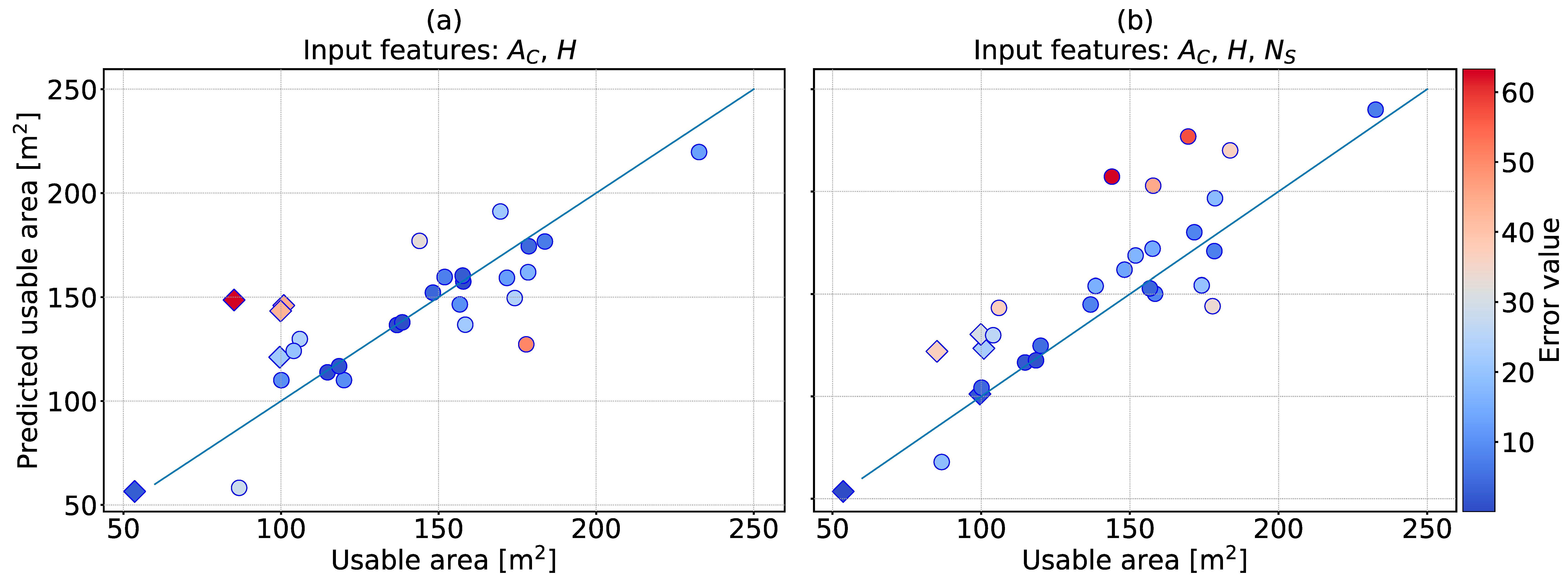
We test two neural networks trained on buildings from architectural bureaus. The first model uses only two input features: covered area and building height, which are readily available in the BDOT10k. The second network also uses the number of stories, which needs to be deduced using Google Street View if absent in the REPR. The comparison of predicted and actual usable areas of 22 Koszalin buildings is presented in Figure 7. The performance metrics are in Table 4. We intentionally left out two extreme outliers found within the dataset: a residential building with over 400 m 2 of usable area and a residential building with 5 stories. Both models predicted the usable areas of those outliers with errors of the order of 50–100%.
Compared to results from the previous section, we see a significant drop in performance resulting from limitations of available training data. At the same time, mean and median absolute errors of the order of 15 m 2 and median percentage error of 15% show that both models achieved a comparable satisfactory accuracy. Surprisingly, the network using only two input features has slightly better performance. Finally, it is interesting to note that the most confusing buildings are different for both models, which hints that both neural networks estimate the usable area in a different way.

4. Discussion

In this work, we extend the machine-learning approach for the estimation of usable area based on topographic data [21] to residential buildings with gable roofs. Such an estimation of the usable area is a challenge that is especially important for Polish real estate appraisers who, due to the incompleteness of the REPR, lack information on usable areas of sold buildings and, therefore, may be prevented from using the most reliable of appraisal techniques—the comparative approach. This challenge is further complicated by a complex legal situation regarding norms used to calculate the usable area in Poland.
Compared to flat roofs studied in Ref. [21], a gable-roof structure creates new challenges for estimation methods, in particular by introducing slants that impact the usable area of the highest floors. For example, changing the knee wall’s height by 1 m, therefore, changing the slope of the roof, causes a change of the building’s usable area by over 15 m 2 . Another issue is the accuracy of airborne laser scanning, which plays a role when measuring the heights of gable-roof buildings (in contrast to flat-roof buildings). In particular, using the Monte Carlo method, we show that while for LoD2 LiDAR data, the mean and worst-case errors in height measurements are around 0.1% and 2-6%, respectively, and can be ignored, the errors introduced by the LoD1 of LiDAR data are not negligible. In particular, as the heights of LoD1 models are determined as a median of heights of LiDAR data points within a building frame provided by BDOT10k, the mean measurement error is close to 50%, and the worst-case error can reach 65%. Therefore, if machine learning methods are applied to LoD1 data on gable-roof or multi-pitched roof buildings, they require a pre-processing of the training dataset to account for these measurement errors. The pre-processing can be done by modifying the building height by subtracting 50% of its gable roof height—effectively its median. This way we ensure that both in our training, and test dataset we define building height the same way. However, for LoD2 LiDAR data, no preprocessing is needed.
After studying the challenges introduced by a gable roof structure, we train the linear regression and neural networks to estimate the usable area of buildings from architectural bureaus of Lipińscy [35] and Archon [36] based on their topographic data. Despite the availability of data on Koszalin buildings, we trained the machine learning models on building designs where we have full knowledge of interiors and of the norm used to calculate its usable area. Thanks to this, the model avoided multiple sources of noise and imperfections that would deteriorate its accuracy. Most importantly, we see that the covered area and the building’s height are not enough to guarantee a high accuracy of trained models. The R 2 coefficients are of the order of 80%, and MedAE around 10 m 2 . Secondly, we see that the neural network performs slightly better than linear regression by every metric. Finally, it is interesting to note that both models, although they have very different natures (e.g., linear vs. non-linear), have very similar predictions on the same test points and struggle the most with the same buildings. Both linear regression and neural network achieved the best performance when provided with a covered area, building’s height, number of stories, and height of the knee wall with a median absolute percentage error of 5 and 3%, respectively. However, the performance increase may not be worth the effort of extracting information on this input feature. An experienced real estate appraiser can use Google Street View to make an educated guess of the knee wall’s height, but this estimate is subjected to a significant error. Therefore, in the following section, we test the machine learning model without taking the knee wall’s height as an input feature. Avoiding a costly input feature such as the knee wall’s height decreases their performance a little, to 6 and 4%, respectively. Such errors are still extremely low and, therefore, acceptable while gaining a smaller number of input features that a real estate appraiser needs to collect. Both models learned correlations present in buildings designed by two architectural bureaus, characterized by modern style. When applied to real buildings constructed between 2020 and 2022, exhibiting different styles, the models have a significantly lower accuracy. The best neural network was then applied to 24 real buildings constructed between 2020 and 2022 in Koszalin, Poland. The information on those buildings comes from the notices on the Koszalin residential buildings’ construction completion sent to the District Construction Supervision Inspector of Koszalin. Therefore, we can rely on reported buildings’ heights, circumventing the problem of the height measurement errors present in LoD1 LiDAR data. The neural network performance in this dataset significantly drops to the median percentage error of 15%. This drop results from limitations of available training data that contains buildings designed in a modern style by two architectural bureaus. At the same time, the median percentage error of 15% shows that neural networks using only the covered area, the height, and optionally the number of stories achieved satisfactory accuracy in estimating the usable area of gable-roof buildings. In particular, such an error is acceptable because administrative courts in Poland regard real estate estimate valuation reports as correct even if they differ by a few percentage points from one to the other. Moreover, according to Polish law, during the estimation of a property’s value, appraisers can use (for comparison) the prices of properties sold by tenders that do not differ more than 20% from average prices on the market for comparison [40]. As a result of the two aforementioned reasons, a median deviation of 15% in the usable area estimation still lets the appraiser stay within the margin of error during the appraisal and identification of similar properties and their respective values.
While using machine learning to estimate a usable area is very promising for the everyday practice of Polish real estate appraisers, we need to note a fundamental limitation of this approach. When the usable area estimation is based solely on topographic data, with no access to interiors, we are unable to take into account any special interior designs, such as a mezzanine, which heavily impact the usable area, regardless of the complexity of the applied model. Moreover, to be fully reliable, this approach requires rich training data. While we believe we have made the next important steps towards creating a useful machine learning tool for real estate appraisers, a final deployment requires gathering much more building data with various design styles, constructed in various years, but with a usable area calculated using the same norm. Due to the complex legal situation regarding Polish norms on usable area calculation, this is an important challenge to overcome.
Next to gathering more data, an interesting extension of this research is the application of a neural network (or a different machine learning model) to estimate the usable area of more complex buildings, e.g., with multi-pitched roofs. Moreover, instead of using tabular topographic data, such a machine learning approach could use three-dimensional models of buildings generated with LoD2 LiDAR data, which is available across the majority of Poland.

Author Contributions

Conceptualization, L.D.; methodology, L.D. and K.C.; software, K.C.; validation, L.D., K.C. and Ż.S.; formal analysis, L.D.; investigation, L.D. and K.C.; resources, L.D., K.C. and Ż.S.; data curation, L.D.; writing—original draft preparation, L.D. and K.C.; writing—review and editing, L.D., K.C. and Ż.S.; visualization, K.C.; supervision, L.D.; project administration, L.D.; funding acquisition, L.D. and Ż.S. All authors have read and agreed to the published version of the manuscript.

Funding

This research received no external funding.

Data Availability Statement

For the building datasets and the code allowing to reproduce all results obtained within this work, please refer to Ref. [39].

Acknowledgments

We thank Anna Dawid for the useful discussions.

Conflicts of Interest

The authors declare no conflict of interest.

Abbreviations

The following abbreviations are used in this manuscript:
BDOT10kDatabase of Topographic Objects (pol. Baza Danych Obiektów Topologicznych)
LiDARLight Detection and Ranging
LoDLevel of Detail
REPRReal Estate Price Register (pol. Rejestr Cen Nieruchomości)
WCSMEWorst-Case Scenario Measurement Error
MMEMean Measurement Error
MAEMean Absolute Error
MedAEMedian Absolute Error
MedAPEMedian Absolute Percentage Error

References

  1. Czaja, J.; Krysiak, Z.; Nowak, R. Analysis of property valuation methods in comparative approach in the aspect of securing the credit liabilities. Finans. Nieruchom. 2005, 2/2005, 16–28. (In Polish) [Google Scholar]
  2. Sawiłow, E. Analysis of the real estate valuation methods in comparative approach. Geod. Rev. 2008, 80, 3–7. (In Polish) [Google Scholar]
  3. Foryś, I.; Kokot, S. Problems with Real Estate Market Analysis. In Microeconomy in Theory and Practice; Scientific Publishing House of the University of Szczecin: Szczecin, Poland, 2001; pp. 175–182. (In Polish) [Google Scholar]
  4. Applied Econometry with Principles; University of Szczecin: Szczecin, Poland, 2006; pp. 25–31. ISBN 83-913389-7-5. (In Polish)
  5. Felcenloben, D. Real Estate Cadastre; Gall: Katowice, Poland, 2009; pp. 29–42. (In Polish) [Google Scholar]
  6. Hycner, R. Basics of the Cadastre; AGH University of Science and Technology Press: Kraków, Poland, 2004; pp. 241–282. (In Polish) [Google Scholar]
  7. Bennett, R. On the Nature and Utility of Natural Boundaries for Land and Marine Administration. Land Use Policy 2010, 27, 772–779. [Google Scholar]
  8. Kaufmann, J. Cadastre 2014: A Vision for a Future Cadastral System; International Federation of Surveyors: Copenhagen, Denmark, 1998; pp. 1–38. [Google Scholar]
  9. Larsson, G. Land Registration and Cadastral Systems; Longman Scientific and Technical: Harlow, UK, 1991; pp. 21–65. [Google Scholar]
  10. Enemark, S. Building Modern Land Markets in Developed Economies. J. Spat. Sci. 2005, 50, 51–68. [Google Scholar]
  11. Stoter, J. Towards a 3D Cadastre: Where Do Cadastral Needs and Technical Possibilities Meet? Comput. Environ. Urban Syst. 2003, 27, 395–410. [Google Scholar]
  12. Kokot, S. Data Quality of Transaction Prices in Real Estate Market. Acta Sci. Adm. Locorum 2015, 14, 43–49. (In Polish) [Google Scholar]
  13. Dawid, L. Analysis of Completeness of Data from the Price and Value Register on the Example of Kołobrzeg and Koszalin Districts in Years 2010–2017. Stud. Res. FEM SU 2018, 1, 91–102. (In Polish) [Google Scholar]
  14. Dawid, L. Analysis of Data Completeness in the Register of Real Estate Prices and Values Used for Real Estate Valuation on the Example of Koszalin District in the Years 2010–2016. Folia Econ. Stetin. 2018, 18, 17–26. [Google Scholar]
  15. Database of Topographic Objects (pol. Baza Danych Obiektów Topologicznych) (BDOT). Available online: https://www.geoportal.gov.pl/dane/baza-danych-obiektow-topograficznych-bdot (accessed on 10 April 2022).
  16. Wężyk, P. (Ed.) Textbook for Participants of Trainings on Using LiDAR Products; Head Office of Land Surveying and Cartography: Cracow, Poland, 2015. (In Polish)
  17. Baldominos, A.; Blanco, I.; Moreno, A.J.; Iturrarte, R.; Bernárdez, Ó.; Afonso, C. Identifying Real Estate Opportunities Using Machine Learning. Appl. Sci. 2018, 8, 2321. [Google Scholar] [CrossRef]
  18. Pinter, G.; Mosavi, A.; Felde, I. Artificial Intelligence for Modeling Real Estate Price Using Call Detail Records and Hybrid Machine Learning Approach. Entropy 2020, 22, 1421. [Google Scholar] [CrossRef]
  19. Kim, J.; Lee, Y.; Lee, M.-H.; Hong, S.-Y. A Comparative Study of Machine Learning and Spatial Interpolation Methods for Predicting House Prices. Sustainability 2022, 14, 9056. [Google Scholar] [CrossRef]
  20. Mora-Garcia, R.-T.; Cespedes-Lopez, M.-F.; Perez-Sanchez, V.R. Housing Price Prediction Using Machine Learning Algorithms in COVID-19 Times. Land 2022, 11, 2100. [Google Scholar] [CrossRef]
  21. Dawid, L.; Tomza, M.; Dawid, A. Estimation of usable area of flat-roof residential buildings using topographic data with machine learning methods. Remote Sens. 2019, 11, 2382. [Google Scholar] [CrossRef]
  22. Benduch, P.; Butryn, K. Legal and standard principles of buildings and their parts usable floor area quantity surveying. In Infrastructure and Ecology of Rural Areas; Polish Academy of Sciences: Cracow, Poland, 2018; pp. 225–238. ISSN 1732-5587. (In Polish) [Google Scholar] [CrossRef]
  23. Benduch, P.; Hanus, P. The Concept of Estimating Usable Floor Area of Buildings Based on Cadastral Data. Rep. Geod. Geoinform. 2018, 105, 29–41. [Google Scholar] [CrossRef] [Green Version]
  24. Budzyński, T. Calculating the Area of Newly-Built Apartments and Buildings According to Uniform Rules. Geod. R. 2012, 84, 31. (In Polish) [Google Scholar]
  25. Buśko, M. Analysis of legal regulations upon estimation of usable area of building and residential unit. Geod. R. 2015, 87, 8–12. (In Polish) [Google Scholar]
  26. Buśko, M. Building contour line in the database of the real estate cadastre in Poland pursuant to applicable laws. Econtechmod Int. Q. J. Econ. Technol. New Technol. Model. Process. 2016, 5, 183–190. [Google Scholar]
  27. Bydłosz, J.; Cichociński, P.; Piotr, P. Possibilities of the Register of Real Estates Prices and Values Restrictions Overcoming Applying GIS Tools. Stud. Inform. 2010, 31, 229–244. (In Polish) [Google Scholar]
  28. Ebing, J. Calculating of Area and Cubic Volume of Facilities with Different Intended Use; Verlag Dashofer Sp. z o.o Publishing House: Ljubljana, Slovenia, 2011; ISBN 978-83-7537-108-6. (In Polish) [Google Scholar]
  29. Polish Committee of Standardization. PN-70/B-02365 Surface Area of Buildings—Classification, Definitions, and Methods of Measurement 1970. Available online: http://rzeczoznawca-zachodniopomorskie.pl/pliki/PN_70_B_02365.pdf (accessed on 22 April 2022). (In Polish).
  30. Polish Commitee of Standardization. PN-ISO 9836:1997 Performance Standards in Building—Definition and Calculation of Area and Space Indicators 1997. Available online: http://rzeczoznawca-zachodniopomorskie.pl/pliki/PN_ISO_9836_1997.pdf (accessed on 20 April 2022). (In Polish).
  31. Regulation of the Minister of Transport, Construction and Maritime Economy of April 25, 2012 on Detailed Scope and Form of a Construction Project. Journal of Laws of 2012, Item 462. Available online: http://prawo.sejm.gov.pl/isap.nsf/DocDetails.xsp?id=WDU20120000462 (accessed on 20 May 2020). (In Polish)
  32. Polish Commitee of Standardization. PN-ISO 9836:2015-12 Performance Standards in Building—Definition and Calculation of Area and Space Indicators 2015. Available online: http://sklep.pkn.pl/pn-iso-9836-2015-12p.html (accessed on 25 May 2020). (In Polish).
  33. Zbroś, D. The Rules for Calculating the Usable Area by Two Current Polish Standards. Saf. Eng. Anthropog. Objects 2016, 3, 19–22. (In Polish) [Google Scholar]
  34. Project W-0426 for Single-Family Detached House of the Spółdzielczy Ośrodek Budownictwa INWESTPROJEKT Design Bureau, Designed by M.Sc. Eng. Arch. Wojciech Kempiński, issued in 1993 (private archive, accessed on 11 April 2022). 11 April.
  35. Lipińscy, M.L. Design Office. Houses Projects. Available online: https://lipinscy.pl/ (accessed on 11 April 2022).
  36. Mendel, B. ARCHON+ Project Office. Available online: https://www.archon.pl/ (accessed on 11 April 2022).
  37. Head Office of Land Surveying and Cartography. Geoportal of National Spatial Data Infrastructure. Available online: https://www.geoportal.gov.pl/ (accessed on 10 April 2022).
  38. QGIS Development Team. QGIS Geographic Information System. Open Source Geospatial Foundation Project. Available online: http://qgis.osgeo.org (accessed on 11 April 2022).
  39. Dawid, L.; Cybiński, K.; Stręk, Ż. GitHub Repository: ML for Usable Area. Available online: https://github.com/kcybinski/ML_for_usable_area_estimation_gable_roofs (accessed on 31 January 2023).
  40. The Ordinance of the Council of Ministers of September 21, 2004 on Real Estate Valuation and Preparation of Valuation Survey. Journal Laws of 2004, Item 2109. Available online: http://prawo.sejm.gov.pl/isap.nsf/DocDetails.xsp?id=WDU20042072109 (accessed on 20 June 2019). (In Polish)
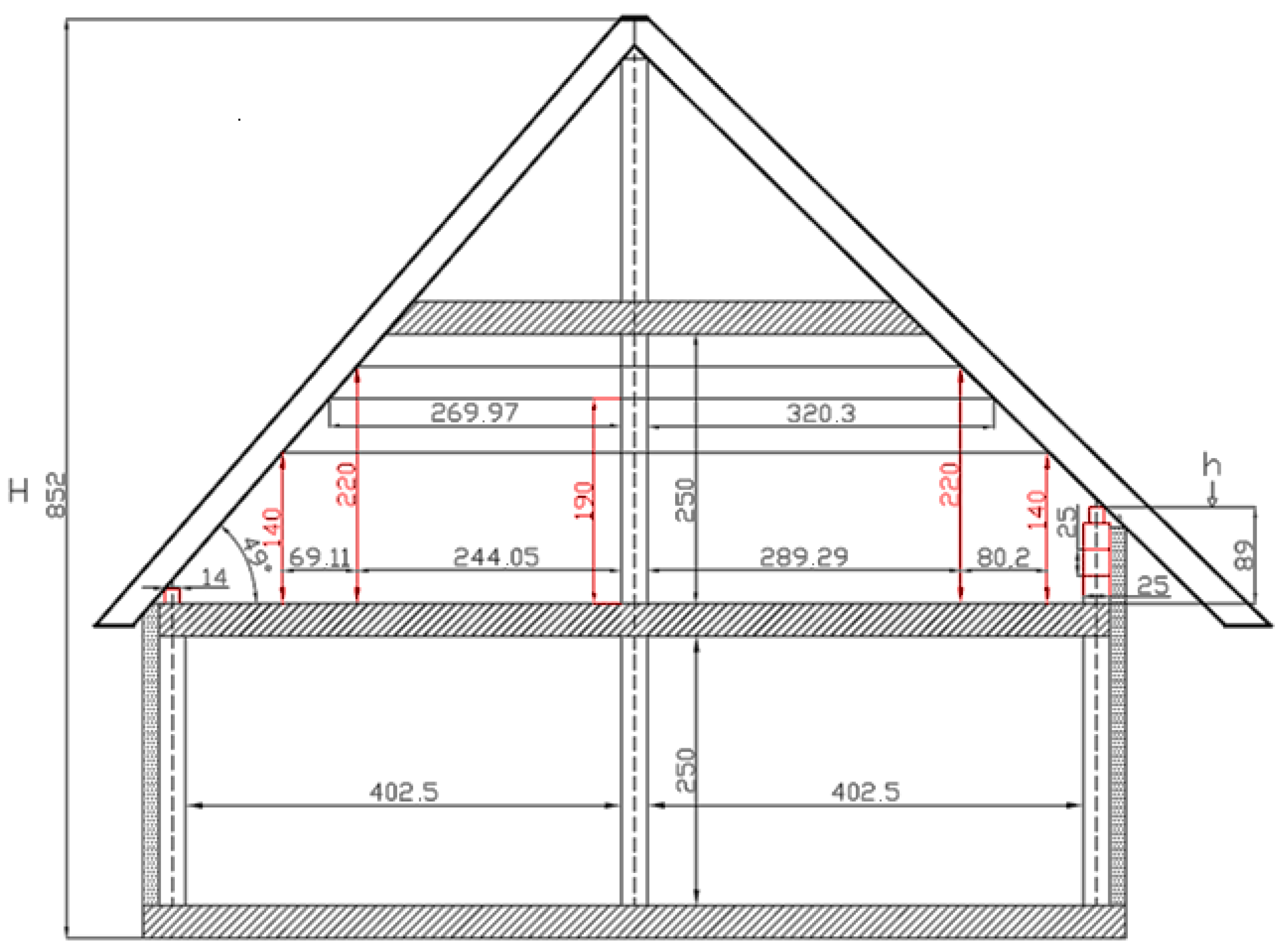
Figure 1. Sketch of the building used to model the relationship between the usable area and the building’s and the knee wall’s heights. H—height of the building, and h—height of the knee wall. The red values marked on the sketch are the verging heights for three used norms described in Section 2.1: 140, 190, and 220 cm.
Remotesensing 15 00863 g001
Figure 2. A render of the roof model we used for our Monte Carlo simulation, with a rendered measurement grid overlaid on top and roof ridge marked in orange. Subplot (a) corresponds to LoD1 measurement grid, with a grid spacing of 1 × 1 m. Subplot (b) corresponds to LoD2 measurement grid, with a grid spacing of 1 3 × 1 4 m. The dimensions we used here are width = 12.44 m, depth = 15.65 m, height = 2 m.
Remotesensing 15 00863 g002
Figure 3. Worst-case scenario measurement error (WCSME) for LoD1 and LoD2 measurements as a function of roof height and roof width.
Remotesensing 15 00863 g003
Figure 4. Mean measurement error (MME) for LoD1 and LoD2 measurements as a function of roof height and roof width.
Remotesensing 15 00863 g004
Figure 5. Predictions of (a) the linear regression and (b) the neural network with 10 hidden neurons of the usable area of buildings from architectural bureaus, with a distinction between one- (diamonds) and two-story (dots) buildings. Input features are the covered area and the building’s height.
Remotesensing 15 00863 g005
Figure 6. Predictions of (a) the linear regression and (b) the neural network with 10 hidden neurons of the usable area of buildings from architectural bureaus, with a distinction between one- (diamonds) and two-story (dots) buildings. Input features are the covered area, the building’s height, and the number of stories.
Remotesensing 15 00863 g006
Figure 7. Predictions of the neural networks with 10 hidden neurons of the usable area of buildings in Koszalin, Poland, with a distinction between one- (diamonds) and two-story (dots) buildings. Input features are (a) the covered area, the building’s height, and (b) also the number of stories.
Remotesensing 15 00863 g007
Table 1. Recorded features of 172 residential buildings from the architectural bureaus and of 24 houses in Koszalin with the range of values present in the dataset.
FeatureSymbolValues
(Design Offices)
Values (Koszalin)
Usable area A U 42.47–217.34 m 2 53.58–438.90 m 2
Covered area A C 47.18–227.60 m 2 66.82–288.39 m 2
Number of stories S N 1–21–5
HeightH4.54–9.16 m6–15.73 m
Knee wall’s heighth0–2.21 mno data
Table 2. Usable area of a top story in a building with a gable roof according to three norms.
Usable Area According to the Norm [m 2 ] 1
h [cm]PN 70ISO 97ISO 2015
1449.9451.5654.7
14 + 2553.055657.9
14 + 2 × 2556.1659.261.1
14 + 3 × 2559.8562.864.9
14 + 4 × 2564.0366.869.2
1 Source: Based on the representative gable-roof building project [34] described in more detail in Section 2.3. Norms: PN 1970 (PN-B-02365:1970), ISO 1997 (PN-118 ISO 9836:1997), ISO 2015 (PN-ISO 9836:2015-12), and h—knee wall’s height.
Table 3. Comparison of estimation accuracy of the linear regression model and the best found neural network models for 34 buildings from architectural bureaus with different input features, as defined in Table 1.
Metric 1Input: A C , HInput: A C , H, S N Input: A C , H, S N , h
LinRegNN
(2-10-1)
LinRegNN
(3-10-1)
LinRegNN
(4-30-1)
R 2 [%]808193979598
MAE [m 2 ]10.279.866.674.094.913.47
MedAE [m 2 ]9.889.315.262.933.303.00
Max error [m 2 ]39.0140.8118.6214.7017.8611.38
Min error [m 2 ]0.410.350.520.280.170.52
MedAPE [%]996453
1 Used metrics: R2 coefficient, mean absolute error (MAE), median absolute error (MedAE), max and min error, median absolute percentage error (MedAPE).
Table 4. Comparison of usable area estimation accuracy of the neural networks for 22 buildings from Koszalin, Poland, with different input features.
Metric 1Input: A C , HInput: A C , H, S N
R 2 [%]6256
MAE [m 2 ]17.2919.40
MedAE [m 2 ]12.4415.42
Max error [m 2 ]63.5063.29
Min error [m 2 ]0.210.03
MedAPE [%]1515
1 Used metrics: R2 coefficient, mean absolute error (MAE), median absolute error (MedAE), max and min error, median absolute percentage error (MedAPE).
Disclaimer/Publisher’s Note: The statements, opinions and data contained in all publications are solely those of the individual author(s) and contributor(s) and not of MDPI and/or the editor(s). MDPI and/or the editor(s) disclaim responsibility for any injury to people or property resulting from any ideas, methods, instructions or products referred to in the content.