UAV LiDAR and Hyperspectral Data Synergy for Tree Species Classification in the Maoershan Forest Farm Region

Abstract

The accurate classification of single tree species in forests is important for assessing species diversity and estimating forest productivity. However, few studies have explored the influence of canopy morphological characteristics on the classification of tree species. Therefore, based on UAV LiDAR and hyperspectral data, in this study, we designed various classification schemes for the main tree species in the study area, i.e., birch, Manchurian ash, larch, Ulmus, and mongolica, in order to explore the effects of different data sources, classifiers, and canopy morphological features on the classification of a single tree species. The results showed that the classification accuracy of a single tree species using multisource remote sensing data was greater than that based on a single data source. The classification results of three different classifiers were compared, and the random forest and support vector machine classifiers exhibited similar classification accuracies, with overall accuracies above 78%. The BP neural network classifier had the lowest classification accuracy of 75.8%. The classification accuracy of all three classifiers for tree species was slightly improved when UAV LiDAR-extracted canopy morphological features were added to the classifier, indicating that the addition of canopy morphological features has a certain relevance for the classification of single tree species.

1. Introduction

Forests are core components of terrestrial ecosystems and play a pivotal role in the global ecosystem [1]. Studying the species composition of forests and spatial distribution of single trees of different species is important for assessing forest habitat quality and forest biodiversity, as well as for formulating rational forest management strategies. Moreover, such analyses are useful for estimating forest productivity, biomass, and carbon stocks [2,3]. With the rapid development of aerospace technology and continuous maturation of sensor technology, remote sensing technology is increasingly being used in forest resource monitoring [4]. The use of remote sensing data for tree species classification can reduce the workload of field surveys, reduce labor costs, and improve the efficiency of forest resource surveys [5,6].

Hyperspectral data in optical remote sensing images are characterized by high spectral resolutions and wide spectral ranges [7], thus providing valuable information for tree species classification. However, hyperspectral data, as a kind of planar remote sensing data, cannot completely reflect the characteristics of the canopy structure in the vertical direction but can provide important information about the canopy surface. In contrast, light detection and ranging (LiDAR) point cloud data can effectively reflect the three-dimensional structural features of the forest canopy, thus compensating for the lack of hyperspectral data [8]. Therefore, the use of LiDAR in combination with hyperspectral remote sensing for tree species classification has recently become a prominent topic of research.

Earlier studies generally relied on LiDAR point cloud data and generated canopy height models (CHMs) for the accurate analysis of canopy boundaries, and the spectral characteristics of vegetation were used for classification [9]. Dalfonse et al. [5] used LiDAR data to segment the crown range of individual trees in the forest and then used hyperspectral data to classify individual tree species in the forest, with the classification accuracy of each tree species between 68% and 95%. Jones et al. [10] combined hyperspectral data and LiDAR to identify eleven key tree species in the Gulf Islands Nature Reserve on the west coast of Canada, with producer’s and user’s accuracies of 95.4% and 87.8%, respectively. Later, studies using LiDAR-extracted height and intensity variables together with spectral data for classification gradually became more popular. Shen et al. [4] collected airborne LiDAR and hyperspectral data in Jiangsu Yushin National Forest Park, selected features by PCA downscaling after shadow-masking the hyperspectral data, selected tree canopy height and structural features based on LiDAR data, and finally used an RF algorithm for single tree species identification with a total accuracy of 86.3%. Sankey et al. [11] combined LiDAR and hyperspectral data to perform tree species identification using a decision tree approach, and the cross-validation results showed that the overall accuracy of tree species identification was 88%. Height and intensity variables extracted by LiDAR can be used to characterize single wood canopies in terms of vertical structure, which has positive implications in tree species classification studies [12].

With the development and maturity of unmanned aerial vehicle (UAV) technology, UAV LiDAR data have been increasingly applied in single tree-scale parameter extraction [13]. Compared to satellite-based or airborne LiDAR, UAV LiDAR usually has the advantages of low scanning height and high point cloud density [14]. Therefore, extracting the 3D structural features of tree canopies using UAV LiDAR is generally accurate [15]. However, previous studies mainly combined hyperspectral data with echo height and intensity variables from LiDAR-extracted point clouds for classification [16], and LiDAR-extracted canopy morphology has been rarely applied in tree species classification.

In summary, tree species classification based on multisource remote sensing is an important research topic in forestry remote sensing. However, the morphological characteristics of single tree crowns, namely, the parameters describing the shape, size, and structure of a crown [17], have rarely been used in the classification of tree species in previous studies. Therefore, in this paper, we used UAV LiDAR and hyperspectral data combined with machine learning algorithms to explore the scientific and synergistic application of multisource remote sensing data for tree species classification at the single tree scale by comparing the classification effects of multiple schemes and quantitatively evaluating the application potential of UAV LiDAR-extracted three-dimensional canopy parameters in single tree species classification.

2. Materials and Methods

2.1. Study Area and Data Acquisition

The study area was the Maoershan Forest Farm, Shangzhi, Heilongjiang Province, Northeast China, ranging from 127°18′0″ to 127°41′6″E and 45°2′20″ to 45°18′16″N, with an average elevation is 300 m, maximum elevation is 805 m, and average slope of 10° to 15°. It is part of the western Xiaoling remnant of the Zhang Guangcai Ridge of the Changbai Mountain System, which has a mid-temperate continental monsoon climate. It is a typical natural secondary forest area in the mountains of eastern Northeast China, with the main vegetation type being temperate mixed coniferous forests [18]. The main species are white birch (Betula platyphylla), Manchurian ash (Fraxinus mandshurica), larch (Larix gmelinii), Ulmus (Ulmus pumila), mongolica (Quercus mongolica Fisch.), Korean pine (Pinus koraiensis Sieb.), maple (Acer pictum Thunb), and Amur linden (Tilia amurensis Rupr.).

In this study, the sample plot survey data were collected in August 2019. Typical mixed coniferous forests were selected in the study area, 100 m × 100 m sample plots were established, and subplots were set at 20 m intervals in the sample plots, for a total of 25 subplots (as shown in Figure 1). Within each subplot, the tree diameter at breast height (DBH) of all trees with a diameter greater than 5 cm was measured using a tape measure, tree height was measured using a Vertex IV instrument with a height resolution of 0.1 m (Haglöfs, Sweden), canopy width was measured in four directions using a steel tape, and the species of each tree was recorded. In addition, the absolute positions of the four corners in each subplot were marked using a real-time kinetic (RTK) GNSS (UniStrong G10A, Beijing, China) with a positioning error of approximately 0.1 m. The coordinates of each tree were recorded using a handheld laser rangefinder by measuring the relative position of each tree in relation to the edge of the subplot. In total, 1372 trees were measured among the sample plots. Considering the number of plants, the main tree species in the forest were white birch, Manchurian ash, larch, Ulmus, and mongolica, with small numbers of other tree species, such as Korean pine and Amur linden.

The UAV LiDAR data used in this study were collected in August 2019. The scanning device was a Pegasus D200 UAV platform with an ultralight RIEGL mini VUX-1 UAV LiDAR scanner (10 mm survey-grade accuracy). The UAV was flown in cross strips at an altitude of 80 m and speed of 5 m/s, with 80 m of lateral overlap between strips. The scanning frequency of the LiDAR pulse was 105 Hz, the scanning speed was approximately 100 times/s, each laser beam produced up to 5 echoes, and the average point density of the point cloud was 243.5 points/m². In addition to the laser sensor, the UAV platform also included a GNSS antenna, a high-precision inertial measurement unit (IMU), and a high-speed storage control unit.

The hyperspectral data were collected in September 2021. The data were obtained by scanning forest stands with a DJI M600 UAV carrying an ITRES MicroCASI-1920 hyperspectral camera. The camera had a lateral scan width of 1920 pixels and field of view of 36.6°. The UAV flew at a relative altitude of 300 m, with a flight rate of approximately 5 m/s. The final acquired hyperspectral image had a ground resolution of 0.1 m. The sensor spanned 288 bands with a spectral range of 400 to 1000 nm and spectral resolution of approximately 5 nm. To reduce band redundancy, the hyperspectral images were resampled into 96 bands (spectral width of 6.3 nm) by the data provider using the Bi-section method in RCX software (ITRES Research Ltd., Calgary, Canada). The hyperspectral images used in this study were geometrically and atmospherically corrected, so no further corrections were needed.

Although there was a time lag between the collection of LiDAR and hyperspectral data, both were collected during the growing season, and the spectral information associated with a single tree species remained relatively stable during the same growing season relative to seasonal changes. Moreover, no human activities, such as logging, or natural disturbances, such as fire, pest issues, or diseases, occurred in the study area during the data collection period. Therefore, we assumed that the tree species and distribution within the sample plot did not change. In general, temporal differences have a small effect on the results of single tree species classification.

2.2. LiDAR Data Preprocessing

The preprocessing of raw LiDAR data includes aerial strip stitching, noise removal, digital elevation model (DEM) and CHM generation, elevation normalization for point clouds, and single tree segmentation. The CHM is an important model for LiDAR remote sensing in forestry applications and can be used to describe the horizontal and vertical distribution of the canopy to obtain an accurate canopy profile [19]. CHM-based single tree segmentation can be used to quickly identify canopy vertices and contours at low cost. In this study, the hole-filling algorithm proposed by Khosravipour et al. (2016) was used to generate a hole-free CHM for normalization of point clouds [20]. The spatial resolution of CHM was set to 0.3 m based on the density of LiDAR point clouds and the minimum canopy width of a single tree, which was chosen to ensure a certain segmentation accuracy and avoid excessive differences in the spatial resolution of hyperspectral images [21]. The marker-controlled watershed segmentation algorithm was used to segment single trees in the CHM and obtain single tree canopy boundaries and structural parameters in the sample plot [22]. The measured single tree positions and crown width were used as references to evaluate the single tree segmentation results. Based on the results of single tree segmentation, a single tree point cloud was extracted from the single tree locations and canopy boundaries to further calculate the morphological characteristics of the single trees in the canopy.

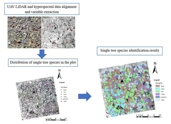
2.3. Image Alignment and Single Tree Matching

Before extracting single tree features, the hyperspectral and LiDAR data were first aligned. Specifically, in this study, the hyperspectral images were aligned for use in the CHM based on the CHM images within the sample site boundary as references. Since the sample site was a forested area, there were no landmarks that could be used for alignment. Therefore, forest gaps with obvious shape, size, and location were used as the basis for alignment and obvious single trees around the forest gaps were used as the control points for the relative alignment of different images by visual interpretation, with the position error controlled within 0.5 image elements.

The positions of the measured single trees were aligned with the corresponding positions in the CHM images, and then the LiDAR-identified tree crowns were matched with the measured single trees according to the crown positions. According to the specific conditions of the study area, if the height error between a measured single tree and a matched LiDAR-identified single tree was less than 30%, the tree was classified as a 1:1 matching single tree; otherwise, it was rejected [16].

The accuracy of single tree matching was evaluated using producer’s accuracy (PA) and user’s accuracy (UA). The specific formulae are as follows:

$$\mathrm{PA}=\frac{\mathrm{M}}{{\mathrm{N}}_{\mathrm{a}}}\times 100\%$$

(1)

$$\mathrm{UA}=\frac{\mathrm{M}}{{\mathrm{N}}_0}\times 100\%$$

(2)

where M is the number of 1:1 matched individual trees, ${\mathrm{N}}_{\mathrm{a}}$ is the number of measured canopies in the plot, and ${\mathrm{N}}_0$ is the number of detected canopies obtained from individual tree splits.

2.4. Feature Extraction and Feature Filtering

2.4.1. Extraction of Hyperspectral Features

In this study, the raw bands of hyperspectral data, minimum noise fraction-transformed and principal component-transformed variables, and vegetation index were used as feature variables for the classification of single tree species. Specifically, when selecting the original band features, we considered the fact that bands with similar wavelengths would display multicollinearity, thus reducing the classification accuracy. From the original 96 bands, 16 bands were selected as classification variables at fixed spectral band intervals. The principal component variables were selected from those with a variance contribution of 90% or more, and the minimum noise fraction variables were extracted from those with a signal-to-noise ratio greater than 3 after minimum noise fraction transformation. The specific spectral feature variables are shown in

Table 1. List of spectral features.

Feature Type	Feature Name	Description
Original waveform	B4, B10, B16, B22, B28, B34, B40, B46, B52, B58, B64, B70, B76, B82, B88, B94	Original waveform
Statistical transformation of variable characteristics	PCA1–PCA3	Obtained from the whole original waveform by principal component transformation
	MNF1–MNF4	Obtained from the whole original waveform by minimum noise fraction transformation

Note: B_x is the reflectance of the x waveband.

and

Table 2. List of vegetation indices.

Vegetation Index	Variable Description
Normalized vegetation index (INDV)	${\mathrm{I}}_{\mathrm{NDV}}=\frac{{\mathrm{B}}_{\mathrm{nir}}-{\mathrm{B}}_{\mathrm{red}}}{{\mathrm{B}}_{\mathrm{nir}}+{\mathrm{B}}_{\mathrm{red}}}$
Ratio vegetation index (RS)	${\mathrm{R}}_{\mathrm{S}}=\frac{{\mathrm{B}}_{\mathrm{nir}}}{{\mathrm{B}}_{\mathrm{red}}}$
Red edge normalized vegetation index (IRENDV)	${\mathrm{I}}_{\mathrm{RENDV}}=\frac{{\mathrm{B}}_{39}-{\mathrm{B}}_{34}}{{\mathrm{B}}_{39}+{\mathrm{B}}_{34}}$
Atmospheric impedance vegetation indices (IARV)	${\mathrm{I}}_{\mathrm{ARV}}=\frac{{\mathrm{B}}_{\mathrm{nir}}-(2{\mathrm{B}}_{\mathrm{Red}}-{\mathrm{B}}_{\mathrm{blue}})}{{\mathrm{B}}_{\mathrm{nir}}+(2{\mathrm{B}}_{\mathrm{Red}}-{\mathrm{B}}_{\mathrm{blue}})}$
Enhanced vegetation index (IEV)	${\mathrm{I}}_{\mathrm{EV}}=2.5\frac{{\mathrm{B}}_{\mathrm{nir}}-{\mathrm{B}}_{\mathrm{red}}}{{\mathrm{B}}_{\mathrm{nir}}+6{\mathrm{B}}_{\mathrm{red}}-7.5{\mathrm{B}}_{\mathrm{red}}+1}$
Vogelman red edge index 1 (Vog1)	${\mathrm{V}}_{\mathrm{og}1}=\frac{{\mathrm{B}}_{38}}{{\mathrm{B}}_{36}}$
Vogelman red edge index 2 (Vog2)	${\mathrm{V}}_{\mathrm{og}2}=\frac{{\mathrm{B}}_{37}-{\mathrm{B}}_{39}}{{\mathrm{B}}_{35}+{\mathrm{B}}_{36}}$
Modified ratio vegetation index (RMS)	${\mathrm{R}}_{\mathrm{MS}}=\frac{{\mathrm{B}}_{39}-{\mathrm{B}}_6}{{\mathrm{B}}_{34}-{\mathrm{B}}_6}$
Anthocyanin reflex index 1 (Iar1)	${\mathrm{I}}_{\mathrm{ar}1}=\frac{1}{{\mathrm{B}}_{18}}-\frac{1}{{\mathrm{B}}_{34}}$
Structural insensitive pigmentation index (ISIP)	${\mathrm{I}}_{\mathrm{SIP}}=\frac{{\mathrm{B}}_{44}-{\mathrm{B}}_6}{{\mathrm{B}}_{44}+{\mathrm{B}}_{31}}$

Note: B_nir, B_red, and B_blue are the average values of reflectance of all bands in the near-infrared (36 bands, 777.516–1001.698 nm), red (24 bands, 615.42–765.05 nm), and blue (7 bands, 428.383–472.018 nm) wavelength ranges, respectively, and Bx is the reflectance of the x band.

.

2.4.2. Extraction of LiDAR Features

In this study, parameters such as height, intensity variables, and leaf area index from LiDAR data were likewise extracted as classification features to explore the effect of the inclusion of LiDAR variables on the classification results. The height variables included the mean absolute deviation, canopy height, height percentile, interquartile spacing, mean, standard deviation, variance, minimum, median, maximum, coefficient of variation, skewness, and kurtosis. A total of 18 variables were included. The intensity variables included the mean absolute deviation, intensity percentile, mean, standard deviation, variance, minimum, median, maximum, coefficient of variation, skewness, kurtosis, cumulative percentile, and interquartile range. A total of 17 variables were included. Additionally, the height and intensity percentile displayed covariance in the 5% to 10% range [23]. Therefore, in this study, height and intensity percentiles of 25%, 50%, and 75% were extracted at 25% intervals.

2.4.3. Extraction of Canopy Morphological Features

To investigate the influence of canopy morphological characteristics on the classification of single tree species, three parameters related to canopy morphology were extracted using UAV LiDAR data in this study: the canopy rate index (R_Ci), crown rate index (R_CSi), and canopy volume ratio (R_VH) [24]. The data obtained were standardized prior to classification to reduce the impact on classification due to differences in values for different attributes [25]. Three tree canopy morphological characteristics were calculated as follows:

L_Ci = V_c/A_C

(3)

R_Ci = L_Ci/H

(4)

R_CSi = L_Ci/W_C

(5)

R_VH = V_C/H

(6)

where H is the detection height; W_C is the detection crown width; A_C is the detection crown area; V_C is the detection crown volume; and L_Ci is the detection crown length index.

2.4.4. Filtering of Feature Variables

In this study, the results of the out-of-bag (OOB) data test with a random forest model were used to rank and filter the significance of the variables [26]. The principle of the OOB test is to assess the accuracy of a classifier by using data that are not extracted as the test sample at each extraction iteration in the random forest model. Each classification parameter was also separately replaced with a random number to compare its effect on the classification results, from which the importance of each variable was obtained [27]. In this study, the mean decrease in accuracy (MDA) was used as a measure of the importance of the variable, indicating the decrease in classification accuracy after replacing the variable with a random number; the larger the value, the greater the impact on the classification results. According to the results of the OOB test, the variables with low importance were screened over several cycles until a combination of variables with sufficient accuracy was obtained.

2.5. Classification Scheme

In this study, five tree species, namely, white birch, Manchurian ash, larch, Ulmus, and mongolica, were used as taxonomic objects in the sample plot. There were too few of the other species in the sample plots to effectively distinguish the trees between the training and test sets; therefore, they were not used as classification targets. In this study, a total of 12 schemes were designed for the classification of single tree species, depending on the data source (hyperspectral, LiDAR, or both), classifier (random forest, support vector machine, or BP neural network), and whether the morphological features of the canopy extracted from LiDAR data were included. Schemes 1, 3, 5, 7, 9, and 11 corresponded to schemes 2, 4, 6, 8, 10, and 12, which were used to compare the advantages and disadvantages of different machine learning classifiers for single tree species classification. Schemes 1 to 8 were used to compare the differences between a single data source and multisource remote sensing classifications, and schemes 10 to 12 were used to investigate the influence of canopy morphological characteristics on the classification results relative to schemes 7 to 9. The specific classification schemes are shown in

Table 3. Brief descriptions of the classification schemes.

Program	Classifier	Variable Group
1	Random forest	Spectral features
2	BP neural network	Spectral features
3	Support vector machine	Spectral features
4	Random forest	LiDAR features
5	BP neural network	LiDAR features
6	Support vector machine	LiDAR features
7	Random forest	Spectral features + LiDAR features
8	BP neural network	Spectral features + LiDAR features
9	Support vector machine	Spectral features + LiDAR features
10	Random forest	Spectral features + LiDAR features + canopy morphological characteristics
11	BP neural network	Spectral features + LiDAR features + canopy morphological characteristics
12	Support vector machine	Spectral features + LiDAR features + canopy morphological characteristics

.

2.6. Classification and Accuracy Evaluation of the Machine Learning Algorithms

To ensure a balanced distribution of each tree species in the training and test samples, we used stratified sampling to divide the samples into five groups and evaluated the classification effects of different classifiers based on different samples and variables using a 5-fold cross-validation test. The classification results for different samples were analyzed to compare the differences in classification accuracy among different classifiers and between different samples. The differences are discussed below. Finally, LiDAR-extracted canopy morphological features were added to the classifiers and the model was tested in the same way to compare the differences in classification results before and after the addition of these variables and evaluate the impact of these parameters on the accuracy of single tree species classification. In this study, the following four metrics were used to evaluate classification accuracy: the producer’s accuracy (PA) and user’s accuracy (UA) for each class and the overall precision (OA) and kappa coefficient (I_kappa) of the model. Both classifiers were constructed in R language. The metrics were calculated as follows:

$$\mathrm{PA}=\frac{{\mathrm{X}}_{\mathrm{ii}}}{\mathrm{N}}\times 100\%$$

(7)

$$\mathrm{UA}=\frac{X_{ii}}{X_{+i}}\times 100\%$$

(8)

$$\mathrm{OA}=\frac{X_{ii}}{X_{i+}}\times 100\%$$

(9)

$${\mathrm{I}}_{\mathrm{kappa}}=\frac{\mathrm{N}{{\displaystyle \sum }}_{\mathrm{i}=1}^{\mathrm{r}}{\mathrm{X}}_{\mathrm{ii}}-{{\displaystyle \sum }}_{\mathrm{i}=1}^{\mathrm{r}}\left({\mathrm{X}}_{\mathrm{i}+}{\mathrm{X}}_{+\mathrm{i}}\right)}{{\mathrm{N}}^2-{{\displaystyle \sum }}_{\mathrm{i}=1}^{\mathrm{r}}\left({\mathrm{X}}_{\mathrm{i}+}{\mathrm{X}}_{+\mathrm{i}}\right)}$$

(10)

where X_ii is the total number of test samples of tree species of category i with correct classification results; X_+i is the total number of test samples identified as tree species of category i; X_i+ is the total number of test samples of tree species of category i; N is the number of test samples; and r is the number of single tree species.

3. Results

3.1. Image Matching and Single Tree Segmentation

Due to the high density of the sample stands, tree canopies may shade each other, resulting in incomplete canopy detection for low single trees and poor single tree division. Therefore, dead and shaded low trees were culled in this study before single tree matching, and a total of 854 single trees remained after culling. Comparing the point cloud segmented single trees with the measured single trees revealed that the tops of the trees were close to each other, the crowns overlapped, and tree height was within 30% error, indicating them to be a perfect match. A total of 719 perfectly matched single trees were obtained through single tree matching, with a PA of 80.7% and UA of 84.2%. The red box in Figure 2 shows the same forest gap marker, and the figure shows that the two remote sensing datasets were well matched. The locations of the successfully matched single trees in the sample plot are shown in Figure 3. Finally, the samples and numbers used for classification were 258 white birch, 84 larch, 167 Manchurian ash, 60 Ulmus, and 67 mongolica trees.

3.2. Filtering of Feature Variables

The categorical feature variables extracted from the two remote sensing datasets were screened according to the random forest OOB test, and the results are shown in Figure 4. Of these, 12 variables were extracted when only hyperspectral data were used as a single data source, 18 variables were extracted when only LiDAR data were used as a single data source, and 16 variables were extracted when both hyperspectral and LiDAR data were used (Figure 4). The figure shows that when both hyperspectral and LiDAR data were used, the importance of the variables extracted from hyperspectral data was higher than that of the variables extracted from LiDAR data. The spectral features reflected the absorption and reflection of electromagnetic waves of different wavelengths on the canopy surface, thus the spectral features of the vegetation deeply reflected differences in the physical and chemical properties of the different tree canopies, so they were more important than LiDAR features.

When using only hyperspectral data, the most important variables were principal component transform feature 1 and MNF feature 2. This result suggested that the statistical transformation associated with the original band improved the specificity of the classified features and thus the classification accuracy. Among the vegetation indices, the enhanced vegetation index and red-edge normalized vegetation index were of high importance, and these two vegetation indices can effectively reflect the characteristics of vegetation in the red edge band. Among the original bands, the 88th and 94th bands were most important, and the wavelength centers of these two bands were 949 and 961 nm, respectively, which were mainly in the near-infrared band. The reflectance of the near-infrared band varied greatly among the tree species in this study. Among the variables extracted from LiDAR data, the height variables were more important than the intensity variables. The mean echo height, the 50% quantile of echo height, and the 50% quantile of cumulative height were of highest importance when using LiDAR data only. The features from LiDAR data used for tree species classification were mainly the point cloud echo height and echo intensity. The echo height feature reflected differences among different tree species in the vertical direction of the canopy and was therefore of high importance in the classification.

3.3. Classification Results

The classification results for each tree species in the sample plot are shown in

Table 4. Classification results.

Classifier	Data Source		Birch	Larch	Ash	Ulmus	Mongolica	OA	Ikappa
BP Neural Network	Hyperspectral	PA	81.28%	52.58%	71.43%	53.09%	72.22%	69.70%	0.59
		UA	68.73%	60.71%	71.86%	71.67%	77.61%
	LiDAR	PA	60.55%	60.00%	47.26%	27.87%	36.49%	51.49%	0.34
		UA	59.85%	71.43%	41.32%	28.33%	40.30%
	Hyperspectral + LiDAR	PA	89.62%	70.53%	78.53%	56.52%	57.83%	75.82%	0.68
		UA	73.36%	79.76%	83.23%	65.00%	72.73%
Random Forest	Hyperspectral	PA	84.32%	69.41%	66.48%	63.64%	72.06%	73.78%	0.64
		UA	76.83	70.24%	72.46%	70.00%	73.13%
	LiDAR	PA	58.49%	62.11%	50.74%	63.83%	58.54%	57.77%	0.40
		UA	71.81%	70.24%	41.32%	50.00%	35.82%
	Hyperspectral + LiDAR	PA	85.77%	70.65%	72.13%	78.18%	83.61%	78.81%	0.71
		UA	81.47%	77.38%	79.04%	71.67%	76.12%
Support Vector Machines	Hyperspectral	PA	75.29%	77.38%	71.86%	70.00%	73.13%	73.94%	0.65
		UA	83.33%	63.73%	80.00%	49.41%	74.24%
	LiDAR	PA	58.69%	72.37%	45.51%	63.33%	58.21%	56.51%	0.42
		UA	67.26%	59.14%	48.10%	51.35%	50.00%
	Hyperspectral + LiDAR	PA	82.63%	76.19%	71.26%	83.33%	79.10%	78.49%	0.71
		UA	80.75%	70.33%	82.07%	70.42%	81.54%

. The overall accuracy of the multisource remote sensing cooperative classification was significantly higher than that of the classification using a single data source. Compared with that of the classification results using only LiDAR data, the accuracy of multisource remote sensing cooperative classification was improved by 22.24% on average. Compared with that of the classification results using only hyperspectral data, the accuracy of the multisource remote sensing cooperative classification was improved by 5.03% on average. After adding canopy morphological characteristics, the classification results shown in

Table 5. Classification results after adding the canopy profile factor.

Classifier		Birch	Larch	Ash	Ulmus	Mongolica	OA	Ikappa
BP neural network	PA	74.90%	83.33%	81.44%	66.67%	70.15%	76.45%	0.68
	UA	87.39%	66.04%	76.84%	60.61%	71.21%
Random forest	PA	81.85%	82.14%	79.64%	71.67%	77.61%	79.91%	0.73
	UA	84.80%	71.13%	77.78%	82.69%	77.61%
Support vector machines	PA	85.71%	80.95%	67.07%	80.00%	80.60%	79.12%	0.71
	UA	81.62%	76.40%	82.35%	67.61%	78.26%

were obtained. The classification results obtained before and after adding LiDAR-extracted canopy morphological features were compared, and the overall accuracy of the model was improved after adding the canopy morphological features. Additionally, the accuracy of the three classifiers was improved by 0.80% on average. The improvement of the random forest classifier was more obvious, reaching 1.10%, and the support vector machine classifier had the lowest improvement of 0.63%. The importance of the three canopy morphological characteristics is shown in

Table 6. Importance of classification of morphological features of the crown.

Feature	Birch	Larch	Ash	Ulmus	Mongolica	MDA
Rci	0.75%	0.43%	1.36%	0.36%	2.83%	0.92%
Rcsi	0.60%	1.05%	0.17%	1.12%	0.12%	0.54%
RVH	0.88%	0.37%	−0.15%	−0.51%	0.19%	0.39%

, which presents the MDA of the three variables for the classification of different tree species. Among the three canopy morphological characteristics, the canopy rate index was the most important, the crown rate index was the second-most important, and the canopy volume ratio was the least important, leading to confusion in the classification of some tree species (MDA was negative). The box plots of the three canopy morphological features are shown in Figure 5. Clearly, the canopy morphological features extracted in this study differed among species. The interspecific variation of R_Ci was obvious, while R_VH displayed less interspecific variation and more intraspecific variation, as well as more extreme values; therefore, the latter variable was not as effective as the first two in the classification.

By tree species, birch displayed the highest classification accuracy overall, while relatively high accuracies were achieved for larch and Manchurian ash. When using only hyperspectral data for classification, the classification accuracy of birch and mongolica was high, with both the PA and UA exceeding 72% on average. When using only LiDAR data for classification, the classification accuracies of both birch and larch were relatively high, above 60%. However, when LiDAR and hyperspectral data were combined for classification, the highest PA and UA were observed for birch. The classification accuracy of white birch was highest when using LiDAR data with hyperspectral data, with both the PA and UA reaching over 80%. After adding the canopy morphological features, the UA of larch and mongolica improved significantly, and although the PA of both decreased by 4.63% and 1.10% on average, the UA improved by 9.69% and 2.62% on average. Moreover, the PA of birch significantly improved by 6.30%.

In this study, the scheme with the highest classification accuracy, scheme 10, was finally used to classify the tree species in the sample plots, and the classification results are shown in Figure 6.

4. Discussion

By comparing the classification results of different classification schemes, we found that the accuracy of using multivariate remote sensing data for single tree species classification was slightly higher than that achieved with using only a single data source. When using multisource remote sensing data, hyperspectral data provided valuable spectral information and LiDAR data complemented the information related to the vertical structure of the canopy, allowing the classifier to identify the features of individual tree species more adequately and thus achieving increased accuracy [28,29]. By tree species, the classification of birch and Quercus serrata was best when only spectral features were used, with an accuracy of more than 70%. Notably, compared to other species, these two trees were characterized by pronounced spectral specificity and large sample sizes, and similar conclusions were noted in previous studies [30]. The classification accuracy of larch was higher when only LiDAR data were used because larch was the only coniferous species among the five species selected for this study, and LiDAR data well reflect the differences in vertical structure between coniferous and broad-leaved species.

By comparing the classification results of each classification scheme and three potential classifiers, we found that the classification accuracy and kappa coefficient of the BP neural network classifier were lower than those of the random forest and support vector machine classifiers. Theoretically, the classification accuracy of the BP neural network classifier can be improved if the size of the experimental data set is increased [31]. Since the size of the data sample used in this study was relatively small, it was difficult to exploit the advantages of the BP neural network classifier.

The accuracy and reliability of random forest classifiers in single tree species classification applications have mutual strengths and weaknesses compared to support vector machine classifiers. In classification problems, random forest classifiers can provide different interpretations of multiple decision trees, are good at handling high-dimensional data, are easy to train, and exhibit good performance in classification problems. In contrast, support vector machine classifiers are better at capturing key features and are more effective in classification because they require only a small number of support vectors to obtain the overall classification results. It is difficult to optimize the classification results when new features are added if the interspecies differences among the new features are not as obvious as those among the original features.

Comparing the classification results of schemes 10–12 with those of schemes 6–9, it can be seen that the inclusion of canopy morphological features improved the accuracy of single tree species identification by 0.80% on average. Although the height and intensity variables extracted from LiDAR data can reflect the structural properties of single tree canopies in the vertical direction to some extent, it is difficult to describe the morphological characteristics of the canopy as a whole [32]. In contrast, the canopy morphological feature parameters extracted in this study effectively described the overall morphology of the canopy, thus complementing the structural information of the canopy in the vertical direction. The introduction of canopy morphological features can further improve the accuracy of single tree species classification because of the differences in the canopy shape of individual species.

Among the three classifiers, the support vector machine classifier was the least sensitive to the inclusion of canopy morphological features, with an accuracy improvement of only 0.63%. This was because support vector machine classifiers often use a small number of vectors to capture the key samples in classification, thereby obtaining the classification result. The advantage of this approach is that support vector machine classifiers provide an excellent filtering effect in cases with considerable noise, but when new variables are added, a support vector machine classifier may be insensitive to the new information. The canopy morphological parameters selected in this study yielded slightly different results compared to those for the spectral features, so the classification accuracy did not improve much. In contrast, the accuracy of the random forest classifier improved by 1.10% after the canopy morphological features were added to the classifier. This was because the random forest classifier uses multiple decision trees to vote on the classification results. With the addition of new variables, the random forest classifier can effectively capture the morphological differences of different kinds of tree crowns, thus improving the classification accuracy.

In addition, the most significant improvement in larch identification accuracy was observed with the inclusion of canopy morphological feature variables. This was due to the notable variation in canopy shape between conifers and broadleaf trees [33]. However, because of the small morphological differences in the canopies of individual broadleaf trees in the sample plots and the large density of stands in the sample plot with overlapping canopies, the improvement in classification accuracy was small. The canopy point clouds of different tree species are shown in Figure 7.

This study had some limitations. First, the hyperspectral data used in the study were collected 2 years after the field data, which may have led to some differences between the spectral profiles extracted from the remote sensing images and the actual spectra of trees at the sample site. Second, the sample size in this study was small and the number of tree species was not balanced, resulting in the limited classification of some species. These limitations will be addressed in future studies.

5. Conclusions

In this study, we used UAV LiDAR and hyperspectral multisource data combined with machine learning algorithms to explore the results of single tree species classification based on 12 classification schemes. The results showed that the accuracy of multisource remote sensing classification was significantly improved compared with that achieved with only a single data source. The classification accuracy of hyperspectral data was higher than that of LiDAR data when using a single data source. Comparing the classification results of different classifiers revealed that the random forest and support vector machine classifiers yielded similar classification accuracy, and both outperformed the BP neural network classifier. This result indicated that the random forest and support vector machine classifiers provided the best classification results for the sample size in this study. Moreover, the classification accuracy of the random forest classifier was most improved after the canopy morphological features were added to the classifier. Among the classification schemes based on multisource remote sensing data and incorporating canopy morphological features, the BP neural network classifier had the lowest classification accuracy of 76.45% with a kappa coefficient of 0.68, while the random forest classifier had the highest classification accuracy of 79.91% with a kappa coefficient of 0.71. The canopy morphological parameters extracted from UAV LiDAR data effectively improved the recognition accuracy of single tree species, especially in the differentiation of coniferous and broadleaf species, with excellent potential for additional applications in the future.