Abstract
Light Detection and Ranging (LiDAR) has advantages in detecting individual trees because it can obtain information on the vertical structure and even on the lower layers. However, the current methods still cannot detect understory well, because the small trees are often clumped together and overlapped by large trees. To fill this gap, a two-stage network named Tree Region-Based Convolutional Neural Network (RCNN) was proposed to directly detect trees from point clouds. In the first stage, very dense anchors are generated anywhere in a forest. Then, Tree RCNN can directly focus on determining whether an anchor belongs to an individual tree or not and generate tree proposals based on the anchors. In this way, the small trees overlapped by big trees can be detected in the process. In the second stage, multi-position feature extraction is proposed to extract shape features of the tree proposals output in the first stage to refine the tree proposals. The positions and heights of detected trees can be obtained by the refined tree proposals. The performance of our method was estimated by a public dataset. Compared to methods provided by the dataset and the commonly used deep learning methods, Tree RCNN achieved the best performance, especially for the lower-layer trees. The root mean square value of detection rates (RMSass) of all plots of the dataset reached 61%, which was 6 percentage points higher than the best RMSass of other methods. The RMSass of the layers < 5 m, 5–10 m, 10–15 m, and 15–20 reached 20%, 38%, 48%, and 61%, which was 5, 6, 7, and 3 percentage points higher than the best RMSass of other methods, respectively. The results indicated our method can be a useful tool for tree detection.
1. Introduction
Individual tree information is important data for biomass estimation, biodiversity assessments, and forest growth models [1]. Although understory vegetation forms a minor proportion of total above-ground biomass, it still plays important roles in forest ecosystems, forest management, carbon emissions, and so on [2,3]. Traditional forestry survey is time-consuming and laborious [4]. For large-scale and comprehensive forest surveys, optical images or airborne Light Detection And Ranging (LiDAR) point clouds [5,6] have been used. Compared to optical images, LiDAR can directly capture 3D forest structures, which is better adapted for individual tree detection [5]. Moreover, LiDAR can partially penetrate the canopies to get information on the lower layers which is difficult to retrieve in optical images [7].
To detect individual trees from airborne LiDAR point clouds, a number of methods have been proposed. A local maxima filtering algorithm that detects trees by local maxima search windows has been widely used for individual tree detection [8,9,10,11]. The local maxima filtering algorithm can successfully detect trees with clear tops. However, the detection capability of the algorithm is strongly affected by the sizes of the search windows and the smoothing factors [12]. Meanwhile, the shaded tree tops cannot be detected by the algorithm. To reduce the under- and over-segmentation in tree detection, template matching methods detect trees not only by the local maxima but also by the whole canopy shape [13,14,15,16]. The methods also perform well for dominant trees but are incapable of finding suppressed trees whose canopy shapes are not as significant as the dominant trees [16]. Clustering methods such as mean shift, K-means, and normalized cut have also been used for tree extraction [17,18,19]. These methods cluster points based on the distance or density of points and have chances to detect understory trees. However, they are susceptible to the quality of point clouds, especially for closed forests where clusters of dense points often appear within the conjunction areas [16].
While most of the above-mentioned methods have reported relatively satisfactory performance, an international benchmarking project revealed that most of the methods cannot detect understory vegetation well [20]. The most critical reasons for the low performance are that there are few points on the understory vegetation and small trees are often clumped together and overlapped by large trees [21]. To better detect the small trees, hierarchical methods have been proposed. Paris et al. [12] and Yang et al. [4] used the local minima algorithm to extract dominant trees by Canopy Height Model (CHM) or point cloud. Then they detected subdominant trees by analyses of the 3-D spatial profile of the dominant tree crowns. Williams et al. [22] used a graph cut algorithm to detect the tree clusters from raw point clouds and employed crown allometry to refine the clusters. Then, the points of the detected tree clusters were removed from the raw point clouds. The graph cut algorithm was used again for the remaining point clouds. The total detected trees were the combination of the trees detected in the two steps. In these methods, because further segmentation was conducted for the initial segmentation points, a few overlapped small trees were separated from the initial segmentation. However, the final results of the hierarchical methods were dependent on the initial segmentation and detection results [23]. Hamraz et al. [23] separated forest points into three layers by the height histogram of the points and utilized the DSM-based method [24] to detect trees in each canopy layer. However, this approach relied on the assumption that the forest structure was characterized by layers that were separable by planes [12]. Therefore, the detection of trees especially small trees remains a challenge.
Compared to traditional object detection methods, deep learning object detection methods, which have achieved great success, can detect objects in an end-to-end process and are data-driven. Therefore, deep learning methods would hopefully overcome the drawbacks of the above hierarchical methods. Currently, numerous methods, such as Faster Region-based Convolutional Neural Networks (R-CNNs) [25], You Only Look Once (YOLO) [26], RetinaNet [27], Sparsely Embedded CONvolutional Detection (SECOND) [28], PointVoxel-RCNN (PV-RCNN) [29], and PointRCNN [30] have been proposed for 2D (Dimension) or 3D object detection in computer vision. A few deep-learning methods have been applied to tree detection for RGB images. Weinstein et al. [6] used RetinaNet to detect the tree crowns. Zhu et al. [31] proposed an improved light YOLOv4 algorithm for fruit tree detection. Ocer et al. [32] used a Mask R-CNN with the Feature Pyramid Network (FPN) to detect trees. Zamboni et al. [33] investigated a total of 21 methods, including anchor-based (one and two-stage) and anchor-free state-of-the-art deep learning methods for tree detection. The results showed overall deep learning methods can obtain good performance for tree detection from images. Correspondingly, several methods have focused on detecting trees from point clouds by deep learning. Windrim et al. [34] generated bird’s-eye view projection (BEV) images from point clouds and used Faster R-CNN to detect trees from the BEV images. Li et al. [35] used an improved Mask R-CNN to detect trees from the RGB images and CHM. The above methods only used deep learning methods to extract features from raster images, and the 3D structure would be lost in the rasterization. Therefore, these methods were more suitable for extracting dominant trees. Schmohl et al. [36] proposed a 3D neural network that can directly extract features from point clouds. They first used a sparse 3D U-Net for 3D feature extraction. Then for tree detection, the 3D features were flattened to 2D features by three sparse convolutional layers. Finally, the trees were detected by the 2D object detection networks based on the 2D features. Although in the feature extraction process, the 3D structure features were extracted, the detection networks were still 2D in the detection process. By using the methods, the understory trees which were overlapped by overstory trees would be lost in the detection process. To better detect the understory vegetation, similar to [23], Luo et al. [37] sliced the forest into three slices and mapped each slice to a raster image. Then the proposed MCR module was used to extract features from each raster image. Finally, the proposed multi-branch network can automatically combine the features from the raster images of different slices for tree detection. The method still relied on the hierarchical forest structure assumption similar to [23] and the trees cannot be directly detected from point clouds by a 3D detection process. Therefore, how to develop deep learning methods for tree detection from point clouds by 3D detection process still needs to be further researched.
To fill these gaps, we attempt to develop a two-stage deep learning method named Tree RCNN to detect individual trees in forests. In the first stage, very dense 3D anchors which were 3D boxes can be generated anywhere in a forest. The Tree RCNN can directly focus on determining whether an anchor belongs to an individual tree or not and generate the tree proposals which were also 3D boxes based on the anchors. As we can find, this was a complete 3D detection process without hierarchical forest structure assumption, and even the small trees overlapped by big trees can be detected in the process. In the second stage, the tree proposals were refined and the positions of the remaining proposals were the final detected individual tree positions. The performance of Tree RCNN was evaluated through the public dataset named NEWFOR (NEW technologies for a better mountain FORest timber mobilization) [38]. The overall performance and the performance with different tree types and tree heights were evaluated to show the robustness of our method. To further evaluate the performance, our method was compared with the other methods the NEWFOR provided and the current commonly used object detection deep learning methods such as SECOND, PV-RCNN, and PointRCNN. The main contributions of the proposed method can be summarized three-fold.
- Novel 3D anchors were proposed to ensure Tree RCNN can detect trees by 3D features and in a 3D detection process. Additionally, compared with methods without deep learning, Tree RCNN can directly recognize both large and small trees by the anchors without relying on the hierarchical detection process. Compared to anchor-based deep learning methods similar to the Faster R-CNN, very dense 3D anchors can be generated in forests with fewer computations.
- The tree tops are the most representative features of the trees and the local maxima points were used as prior knowledge to generate anchors. The added anchors improved the detection rates of trees by Tree RCNN.
- Motivated by the multi-view 3D object feature extraction [39], multi-position feature extraction was proposed. Compared to extracting features from only one position, extracting features from multi-positions can improve the feature extraction capabilities of Tree RCNN.
2. Materials and Methods
The deep learning object detection methods can be classified into one-stage and two-stage methods. Generally, the detection speeds of one-stage methods are faster than those of two-stage methods, but the detection accuracy of one-stage methods is lower than that of two-stage methods. Therefore, to obtain better accuracy, a two-stage method called Tree RCNN was proposed for individual tree detection.
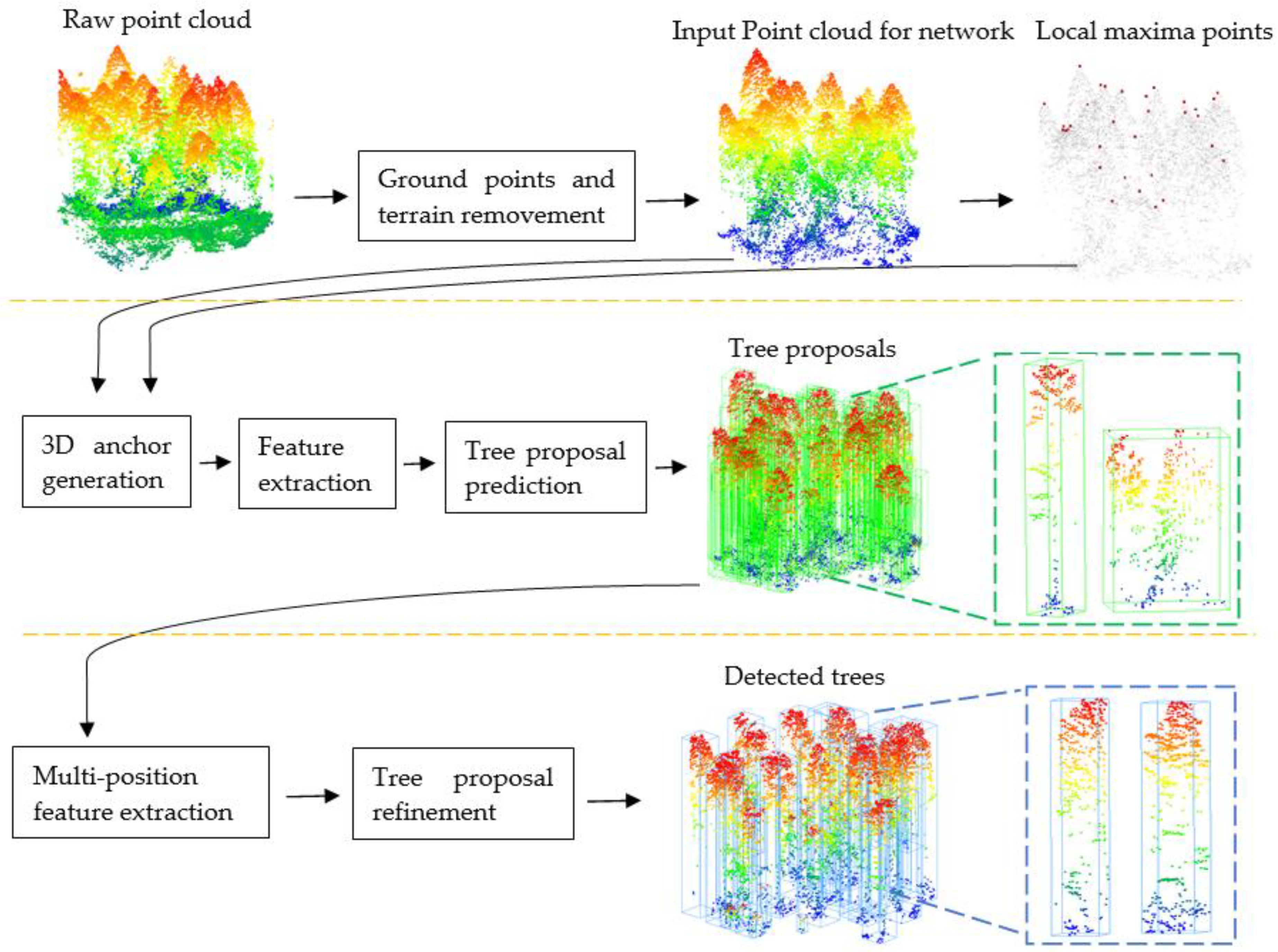
The overall structure of our method is illustrated in Figure 1. The first line is preprocessing. The second line is the first stage which is the 3D proposal generation stage of the Tree RCNN. The third line is the second stage which is the tree proposal refinement stage of the Tree RCNN.
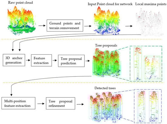
Figure 1.
The Tree RCNN architecture for tree detection. The first line is the preprocessing. The second line is the 3D proposal generation stage. The third line is the tree proposal refinement stage. The green boxes are 3D tree proposals. The blue boxes are the final tree proposals.
Preprocessing was conducted to remove the effect of ground points and terrain for tree detection and provide the local maxima points and bounding boxes of reference trees for the following Tree R-CNN.
The Tree RCNN took a 3D point cloud of a plot after preprocessing and the local maxima points as the input. The bounding boxes of the reference trees were used as labels. In the first stage, 3D anchors were proposed to generate 3D tree proposals which are the green boxes in Figure 1. In the second stage, the multi-position feature extraction was proposed to extract features of the tree proposals. The tree proposals were refined to obtain the final tree proposals based on the features. The final tree proposals shown as the blue boxes in Figure 1 were the output of the Tree RCNN. The positions and heights of detected trees can be obtained based on the refined tree proposals.
2.1. Preprocessing
To prevent the terrain and low vegetation points from affecting the tree detection, the heights of the points were first replaced by the heights which were the relative point heights over the DEM [40]. Then the points lower than 0.5 m in height were removed. Since the height of the lowest tree in the dataset is 1.5 m, the removed points would not affect the shapes of the crowns.
Local maxima points which were extracted through the following three steps [20] were used as prior knowledge for Tree RCNN. First, the CHM with 0.5 × 0.5 m resolution was generated based on the point cloud of a plot. Second, a closing filter with a sliding window of size 3 × 3 pixels was conducted for the CHM. Finally, a local maxima filter with a sliding window of size 3 × 3 pixels was applied to extract the local maxima pixels. The highest point in a local maxima pixel whose value was superior to 5 m was a local maxima point. All the local maxima points were recorded as input for the Tree RCNN.
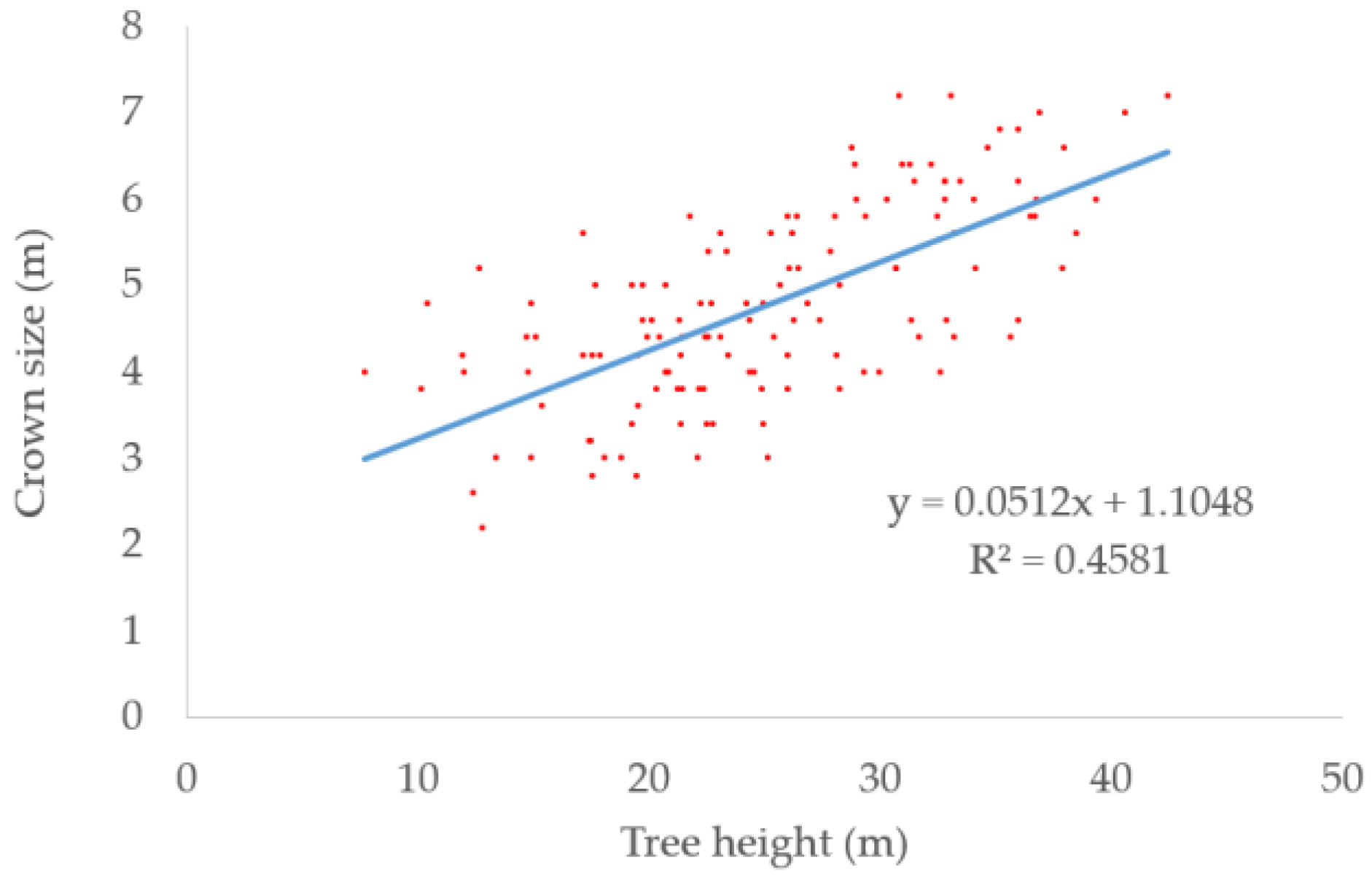
Ground truth bounding boxes of objects are needed for object detection methods. However, the NEWFOR dataset does not provide the crown sizes of the trees, making the accurate bounding boxes unavailable. Meanwhile, because most of the trees overlapped with each other, determining their crown sizes manually is also impossible. Many studies have shown there is a correlation between tree heights and crown sizes [41]. Therefore, we collected the crown sizes and heights of significant trees whose crowns can be easily recognized to establish the regression equation. The crown sizes of all trees can be calculated by the regression equation. After crown sizes were obtained, the ground truth bounding boxes of trees can be generated. Commonly, a coordinate of a 3D bounding box can be parameterized by the center point coordinates, lengths, widths, and heights. Here, because the trees are on the ground, the heights of the bottoms of the bounding boxes were 0. Meanwhile, as the bottoms of the bounding boxes were assumed to be square, the lengths and widths of the bounding boxes were the crown sizes of the corresponding trees. Therefore, the coordinate of a tree 3D bounding box was parameterized as (x*, y*, h*/2, w*, w*, h*) with four parameters. (x*, y*, h*/2) was the center point coordinates. W* was the crown size. H* was the tree height. The bounding boxes of reference trees were used as the ground truth bounding boxes for Tree RCNN to approximately determine the scopes of trees.
2.2. 3D Proposal Generation Stage
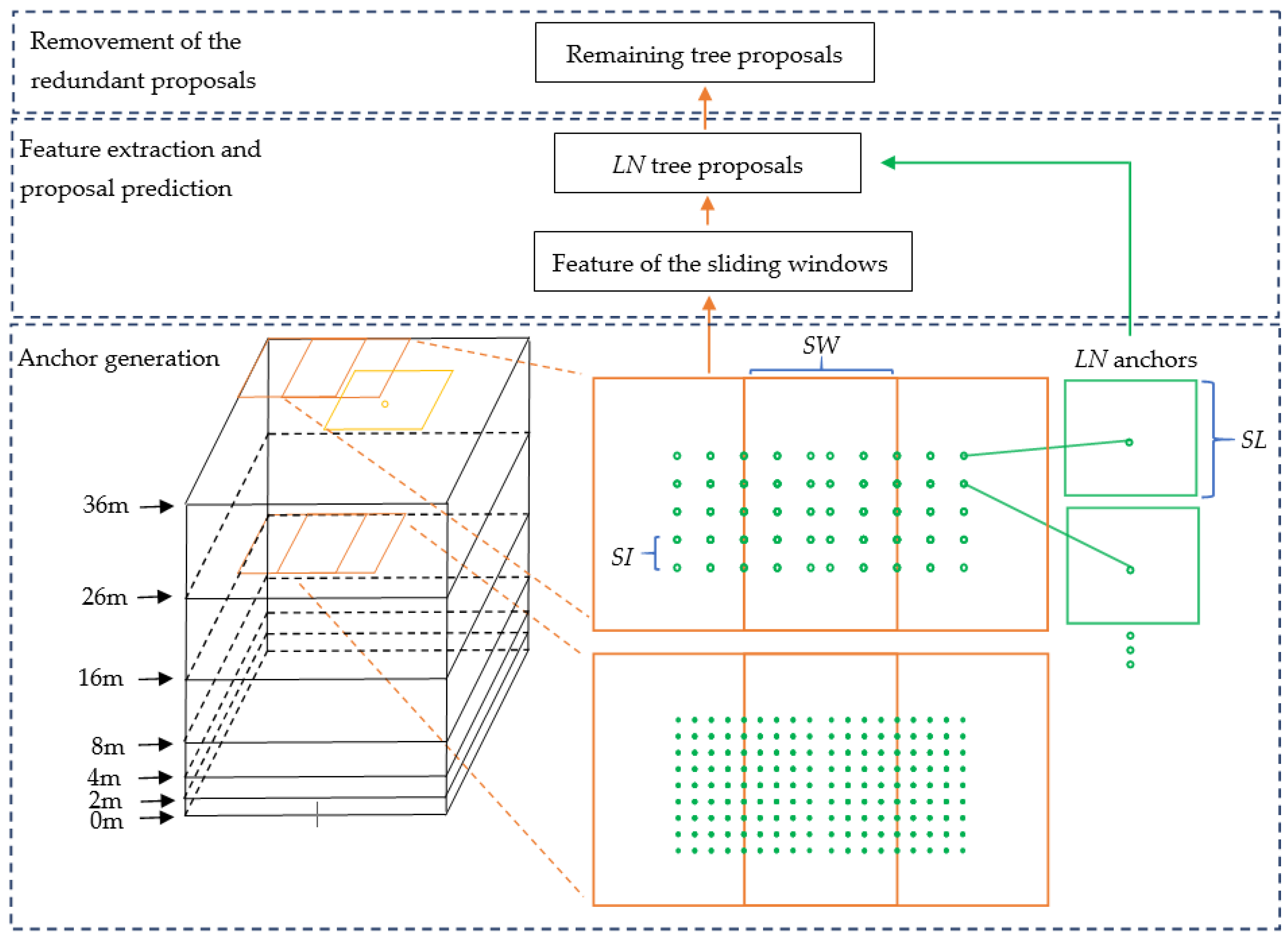
The input of the 3D proposal generation stage was the point cloud of a plot and the local maxima points. The process of 3D proposal generation contained three parts. In the first part, the 3D sliding windows were generated based on the size of a plot. The 3D anchors were generated based on the 3D sliding windows and the sliding windows located at local maxima points. 3D anchor generation was the key part of the stage, which ensured the Tree RCNN can directly detect trees in a 3D detection process. In the second part, the features of all the sliding windows were extracted. The scores and coordinates of tree proposals were predicted by the features and coordinates of anchors. The number of the tree proposals was the same as that of the anchors. In the third part, the Non-Maximum Suppression (NMS) [25] was produced for the prediction proposals to remove the redundant proposals. The remaining proposals were the output of the stage. The process is illustrated in Figure 2. The black boxes are 3D bounding boxes at different height levels of a plot. The orange boxes are sliding windows. The yellow point is a local maxima point and the yellow box is a sliding window located at the yellow point. The green points are dense location indexes. The green boxes are dense anchors. SW is the Stride of the sliding Window. SI is the Stride of the location Index. SL is the Side Length of anchors. LN is the Location index Number.

Figure 2.
Structure of the 3D proposal generation stage. The black boxes are 3D bounding boxes at different height levels of a plot. The orange boxes are sliding windows. The yellow point is a local maxima point and the yellow box is a sliding window located at the point. The green points are dense location indexes. The green boxes are dense anchors. SW is the Stride of the sliding Window. SI is the Stride of the location Index. SL is the Side Length of anchors. LN is the Location index Number.
2.2.1. Anchor Generation
To construct a 3D detection process, inspired by anchor generation in Faster R-CNN, we generated 3D anchors in the forest and recognized the ones belonging to individual trees. In this way, the Tree RCNN can directly focus on the anchors without the hierarchical forest structure assumption. Meanwhile, if the anchors have large overlaps with the small trees, small trees, even overlapped by big trees, can still be detected.
To ensure all trees can be detected, very dense anchors were needed. Direct extension of the anchors from 2D to 3D was not suitable for tree detection due to the huge 3D search space and the irregular format of point clouds. To address the problem, compared to common anchors only associated with scales and aspect ratios, the proposed 3D anchors were additionally associated with dense location indexes in 3D sliding windows.
To generate 3D anchors, the 3D sliding windows should be generated first. The 3D sliding windows were sliding in a 3D box whose bottom was half of the maximum crown size extension of the bottom of a plot’s bounding box. The expansion avoided missing the trees located near the boundary of the plot in detection. To detect different heights of trees, several height levels were set. Uniform height settings would result in too many height layers. The height setting only needed to ensure that the generated anchors had enough height intersections with the ground truth bounding boxes. Therefore, the height levels were proportional. The bottom of a sliding window was set as a square with a side length equaling the maximum crown size in the dataset. The height of the bottom was 0 since the trees are on the ground. The SW in the horizontal plane was half of the maximum crown size. An intersection between the neighboring sliding windows ensured there was at least one sliding window containing most parts of a tree.
The dense 3D anchors were generated based on 3D sliding windows. To put it simply, the dense 3D anchors were named Ad. The heights of the bottoms and tops of the Ad were the same as those of the sliding windows to which the Ad belonged. By using the correlation between tree heights and crown sizes, the SL of the bottoms of Ad were calculated by the regression equation of the crown sizes and heights in preprocessing based on the heights of the anchors. In the top face of 3D sliding windows, the uniform location indexes were further generated as the green points shown in Figure 2. Because there were intersections between two neighboring sliding windows, the location indexes were only generated at the square areas whose centers were the centers of the 3D sliding windows. The Side Lengths of the Square Areas (SLSA) were (round (SW/4/SI)) × 2 × SI. SI was the stride of the location index, which was set to SL/5. Ad were generated at the uniform location indexes in the square areas. For a sliding window, LN uniform locations were generated, and correspondingly LN anchors were generated. LN equaled SLSA × SLSA. Such a small SI made sure the Ad were dense enough.
Local maxima points often corresponded to tree tops. Generating 3D anchors around the positions of local maxima points would make the anchors and the trees have large overlaps, which meant the trees have greater chances of being detected by the anchors. Since the 3D anchors were generated not only by sliding windows but also around the positions of local maxima points as complements, the detection probability of trees was further improved.
The process of generation of 3D anchors around local maxima points was as follows. The 3D anchors around local maxima points were named Al, to simply distinguish them from Ad. For each local maxima point generated from the CHM, a 3D sliding window whose top center was the position of the local maxima point was generated the same way as the sliding window generated above. The yellow box in Figure 2 is an example of a 3D sliding window. The generation of Al for the 3D sliding window was also the same as that of Ad motioned above. The total anchors were a combination of Ad and Al.
2.2.2. Feature Extraction and Proposal Prediction
In the feature extraction process, first, the coordinates of the points in 3D sliding windows were normalized by subtracting the coordinates of the bottom centers of the 3D sliding windows. Then PointNet++ [42], which is a highly used network, was employed to extract shape features from the points in each 3D sliding window.
To classify the tree proposals relative to the anchors, a label should be assigned to each anchor. Since the crowns of the trees are important for tree detection, it is not suitable to use Intersection over Union (IoU) overlap between the volume (IoUv) of an anchor and a ground-truth box. For example, IoUv = 0.5 is a relatively satisfactory value for common 3D object detection. However, if the bottoms of the anchor and the ground-truth box are coincident, IoUv = 0.5 means the anchor height is only half of the ground-truth box height and most of the crowns are not contained in the anchor. As a result, the anchor would not be considered an approximate bounding box of the tree. Therefore, IoUb which expresses the IoU overlap of the bottom areas of two 3D boxes, and IoUh which expresses the IoU overlap of the height of two 3D boxes were used as the additional criteria for label assignment. We assigned a positive label to two kinds of anchors: (1) the anchor with the highest IoUv overlapped with a ground-truth box, or (2) an anchor that has an IoUb higher than 0.65, an IoUh overlap higher than 0.7, and an IoUv overlap higher than 0.4 with any ground-truth box. The other anchors were assigned negative labels.
After the label assignment, the anchors were classified and the coordinates of the tree proposals were predicted by the coordinates of the anchors by minimizing an objective function following the loss in [25] as Equation (1).
where i is the ith anchor. is the score which is the probability of the ith anchor belonging to trees. The ground-truth label is 1 if the anchor is positive, and is 0 if the anchor is negative. is a vector representing the four parameterized coordinates of the predicted bounding box as Equation (2), and is that of the ground-truth box associated with a positive anchor as Equation (3). Variables x, xa, and x* are for the predicted proposal, anchor, and ground-truth box respectively (likewise for y, w, h). The classification loss term Lcls is the focal loss [27]. The bounding box regression loss term Lreg is the smooth L1 loss [43]. The two terms are normalized by the number of anchors Ncls and the number of positive anchors Nreg and weighted by a balancing parameter .
2.2.3. Removement of the Redundant Proposals
Most of the prediction proposals were redundant and to remove the redundant proposals, NMS [25] was conducted for the proposals. To avoid removing the potential treetops, the NMS was separately conducted for the proposals generated by Ad and Al. For the proposals generated by Ad, NMS with IoUv threshold 0.6 and max remaining proposal number threshold 2500 was used. Meanwhile, for the proposals generated by Al, NMS with IoUv threshold 0.6 and max remaining proposal number threshold 5 was used. The NMS was not conducted for all the proposals generated by Al but separately conducted for the proposals generated by each local maxima point. All the remaining proposals were tree proposals in the first stage.
2.3. Tree Proposal Refinement Stage
The second stage used the remaining proposals obtained from the first stage as input. Similar to the first stage, the second stage contained a feature extraction and proposal prediction process which extracted features from points in the remaining proposals and predicted better tree proposals. The following was the process of removing the redundant proposals. The remaining proposals were the output of the second stage, based on which tree positions and heights can be obtained.
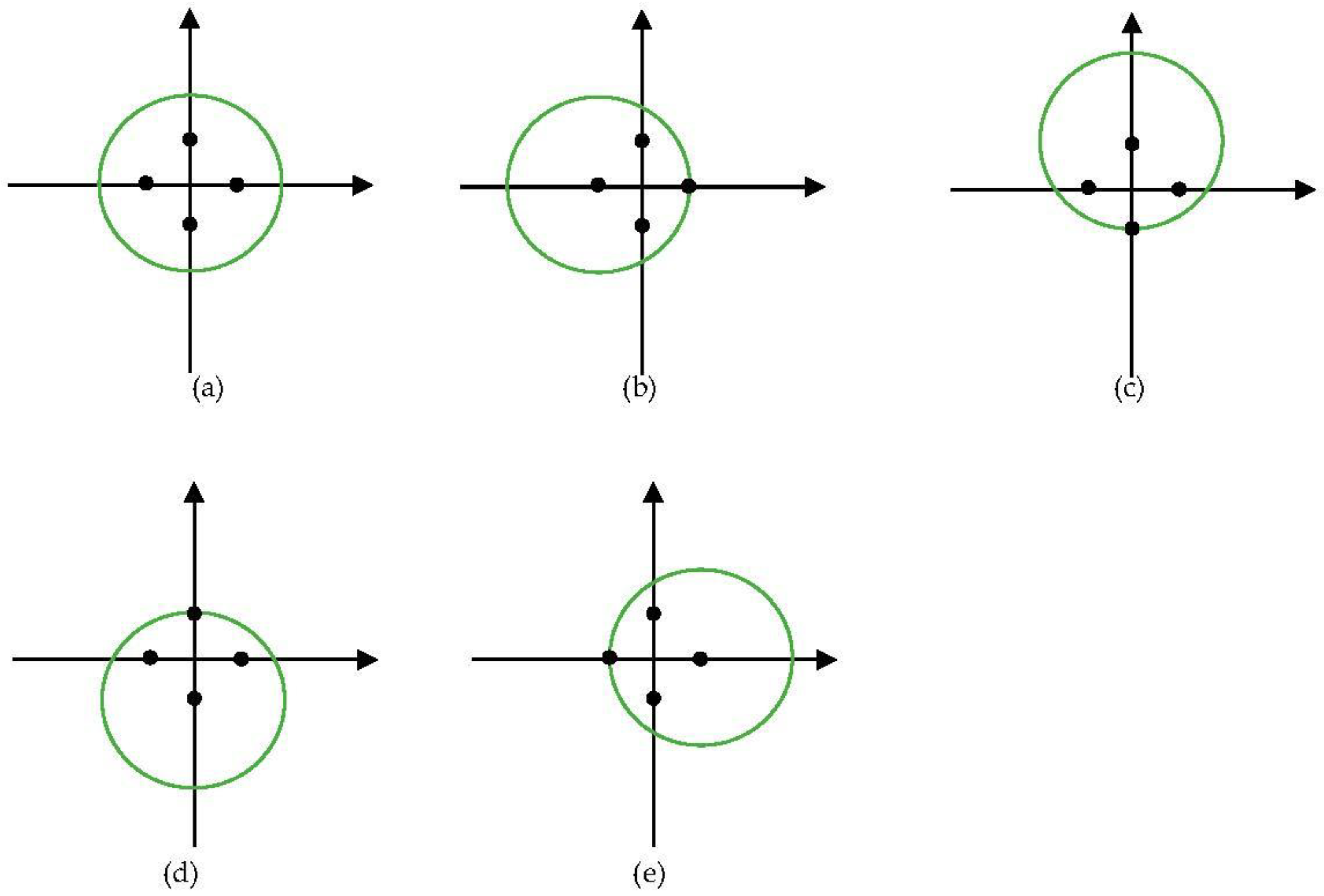
Extraction of features from multi-view can improve the performance of features as shown in the multi-view feature extraction method [39]. Inspired by the methods, a muti-position feature extraction was proposed to extract better features. For point cloud feature extraction, the normalization of the points can be seen as a transformation of the points. Therefore, we used another four positions, i.e., (x, y + w/2), (x, y − w/2), (x + w/2, y), (x − w/2, y), to normalize the points. Figure 3 shows the five views of a tree with five normalizations. The green circles represent trees viewed from the zenith. Black points are the four normalization positions. As five normalized points were obtained, still PointNet++ [42] was used for feature extraction. The points normalized by the center were used as the coordinates of the points input to PointNet++. The other four normalized points were concatenated as the features of the points input to PointNet++.
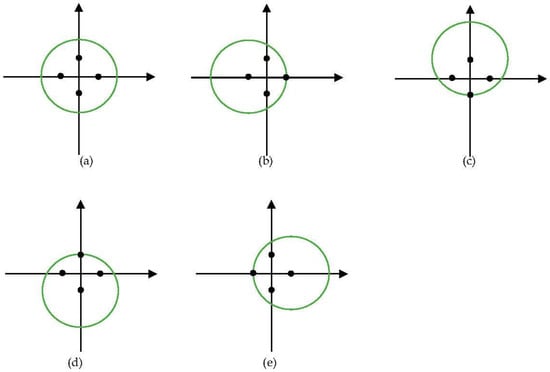
Figure 3.
Views of the five positions of a tree. The green circles represent trees viewed from the zenith. Black points are the four normalization positions. (a) Normalized by center; (b) Normalized by (x + w/2, y); (c) Normalized by (x, y − w/2); (d) Normalized by (x, y + w/2); (e) Normalized by (x − w/2, y).
When feature extraction was finished, we classified the tree proposals output from the first stage and updated the positions of the proposals to obtain refined tree proposals. The label assignment criteria were the same as that in Section 2.2.2. The objective function to obtain the refined proposals was similar to that completed in Section 2.2.2. The difference was that the parameters of the anchors in Equations (2) and (3) were replaced by the parameters of tree proposals output from the first stage.
After proposal refinement, the NMS with tree probability score threshold 0.4 and IoUv threshold 0.4 was used for the refined proposals to remove the redundant. The remaining proposals contained the finally detected trees. The horizontal position of a detected tree was the bottom center position of the corresponding remaining proposals. The height of the detected tree was the height of the highest point in the corresponding remaining proposals.
2.4. Implementation Details
For each plot in the training set, if the number of points was larger than 40,000, we subsampled 40,000 points from the plot as the inputs. The tree height ranged from 1.5 m to 42 m in the dataset. Correspondingly, the height levels of the sliding windows were set to 2 m, 4 m, 8 m, 16 m, 26 m, and 36 m in this paper. For the feature extraction in the two stages, 512 points were randomly sampled as the input to PointNet++. Three set abstraction layers with single-scale grouping [42] (with group sizes 64, 32, 1) were used to generate a single feature vector for position prediction and tree probability estimation. The number of positive and negative labels randomly selected for training was 256 in the two stages. Before training, the horizontal coordinates of the points were randomly rotated by an angle based on the horizontal centroid of the plot and then randomly added by a number between −0.5 m and 0.5 m. The two-stage sub-networks of Tree RCNN were trained together. The total loss was the sum of the loss obtained in the first and second stages. An AdaGrad optimizer [44] was used to train Tree RCNN with a mini-batch size of 1 and a learning rate of 0.0001. The Tree RCNN was implemented on a computer with an NVIDIA GeForce GTX 1080Ti. Python 3.7 was used with the Pytorch1.7.1 deep learning framework. The training process ran 5000 epochs which took about 15 h.
3. Results
3.1. Study Areas
The study areas in this paper were obtained from the NEWFOR project which provided a benchmark dataset and aimed at improving forest management by using new remote sensing technologies such as airborne laser scanning (ALS) [20]. The public parts of the benchmark dataset contained fourteen plots in six areas with different forest types, such as Single-Layered Mixed forest (SL/M), Single-Layered Coniferous forest (SL/C), Multi-Layered Mixed forest (ML/M), and Multi-Layered Coniferous forest (ML/C). The point densities of the point clouds in different areas also varied. The dataset provided the Digital Elevation Model (DEM) of each plot, the Region-Of-Interest (ROI) of each plot, and the positions and heights of the trees in the ROIs. The total recorded tree number in all the ROIs was 1599 with the height ranging from 1.5 m to 44 m. However, there were time gaps between the ALS flight and the field survey in the study areas. The actual tree number in point clouds would be slightly different from the number recorded in the dataset due to the removal or planting of trees. Meanwhile, the tree heights were also different due to tree growth. The details of the dataset are shown in Table 1.

Table 1.
Ground inventory details of the dataset.
3.2. Evaluation Criteria
To evaluate the performance of Tree RCNN for tree detection, a 4-fold cross-validation (CV) approach was used. The plots of the dataset were divided into four folds for the following two reasons. First, the same study areas should be assigned to the same fold. If there is no same study area in both the train and test folds, the generalization ability of Tree RCNN can be better evaluated. Second, each fold should contain a similar number of trees. Finally, the four folds were plot 1, plots (2, 3, 4, 6, 7), plots (5, 8, 9, 10), and plots (11, 12, 13, 14). For the 4-fold CV, three folds were used for training and the other fold for testing. This process was repeated four times to ensure all samples were tested.
The matching and evaluation algorithms that the NEWFOR dataset provided [20] were used to evaluate the performance of Tree RCNN.
After the matching process, the quantitative estimation parameters for each plot are shown below:
Rer (Extraction rate) = NTest/NRef.
Rmr (Matching rate) = NMatch/NRef.
Rcr (Commission rate) = (NTest − NMatch)/NTest.
Ror (Omission rate) = (NRef − NMatch)/NRef.
HMean: Mean horizontal difference of the matching trees.
VMean: Mean height difference of the matching trees.
Where NTest is the Number of detected trees, NRef is the Number of Reference trees, NMatch is the Number of matched trees.
The global quantitative estimation parameters for the dataset are shown as below:
RMSextr: Root Mean Square of Rer.
RMSass: Root Mean Square of Rmr.
RMSH: Root Mean Square of HMean.
RMSV: Root Mean Square of VMean.
RMSCom: Root Mean Square of Rcr.
RMSOm: Root Mean Square of Ror.
3.3. The Regression Results of the Tree Heights and Crown Sizes
We collected 131 significant trees in the dataset for developing the regression equation. The regression equation is shown in Equation (8). The scatter plot of tree heights and crown sizes is shown in Figure 4 and the blue line is the fitted line. The coefficient of determination (R2) reaching 0.46 meant the crown sizes can be approximately calculated by the heights.
where y is the crown size, x is the tree height.
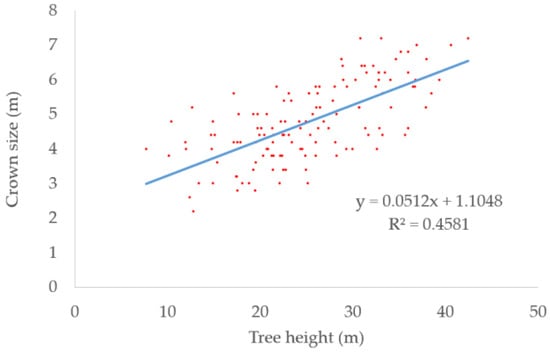
Figure 4.
Scatter plot of tree heights and crown sizes. The blue line is the fitted line.
3.4. Performance of Tree RCNN for Tree Detection
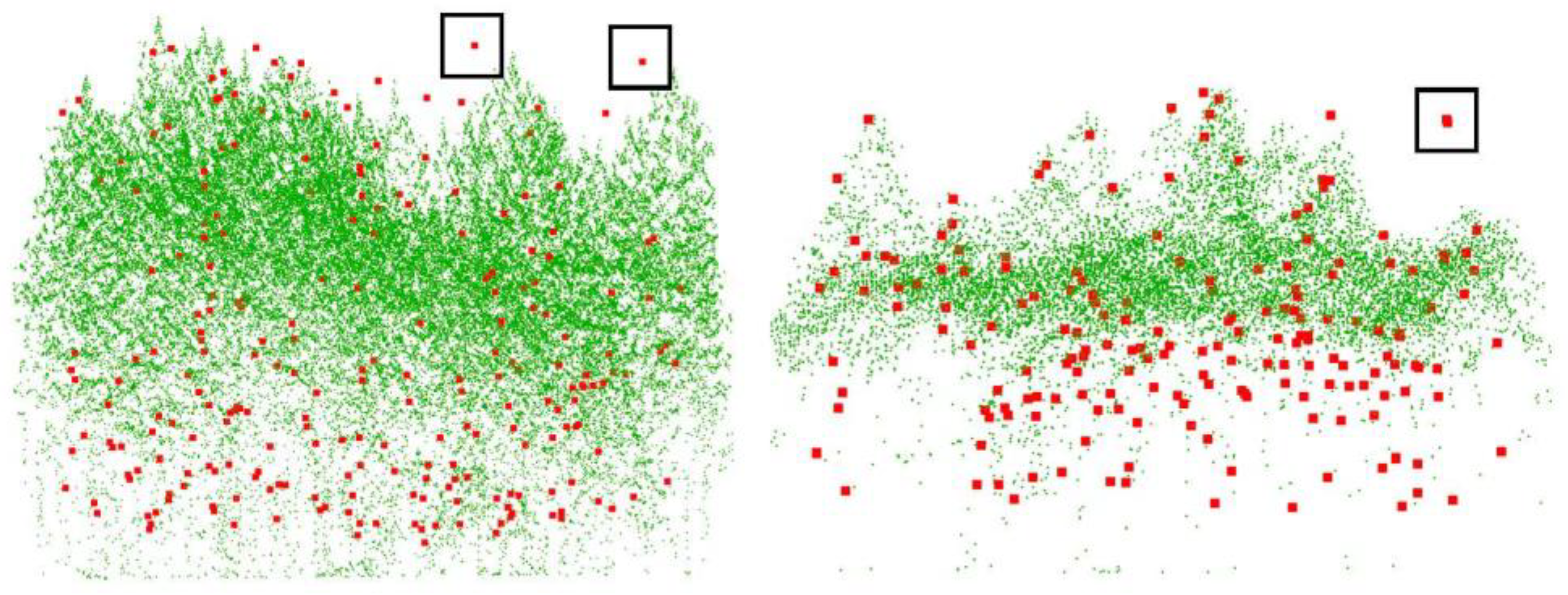
In the ROIs of the 14 plots, there are 1599 reference trees. By using the Tree RCNN, a total of 2194 trees were detected and 913 of them were matched with the reference trees. For each plot, the quantitative estimation parameters are shown in Table 2. The performance of Tree RCNN for different forest types was also estimated and is shown in Table 3. For the 14 plots, there were 11 plots with Rmr greater than 50% and eight plots with Rmr greater than 60%. The best Rmr with a value of 80% was found in plot 6. Meanwhile, the RMSass of different forest types were all larger than 49% and the RMSass of SL/C reached 72%. All the results showed Tree RCNN can detect most of the trees in the dataset and perform well in most of the plots with different forest types. There were still three plots with Rmr less than 50%. The bad performance was mainly due to the forest type and point density. As we can find in Table 3, the trees were detected better in the SL forest than ML forest. For the ML forest, LiDAR can hardly penetrate the crowns of overstory vegetation, and plots 7 and 10 are examples shown in Figure 5. In Figure 5, the green points are tree point clouds, and the red points are reference tree top positions. For the understory vegetation in Figure 5, there were only a few or even no green points around the red points. Detecting lower-layer trees from such a few points would be an unrealistic task. Therefore, the Rmr for plot 10 was only 40%. Even worse, the point densities of plots 6, and 7 were much higher than that of other plots. As there was no similar sample plot with high point density in the training process, the deep learning method would not produce good results. Therefore, plot 7 had the worst Rmr. Rer can affect both Rmr and Rcr. Although high Rer induced high Rmr, too high Rer would induce high Rcr, which meant the detected trees contained too many unexpected misrecognized trees. There were five plots with Rer larger than 150%. Heigh Rer was mainly due to the overfitting of the understory vegetation. In the training process, the distributions of the points of the small trees which did not have the characteristics of a tree were forced to be fitted by the network. There were many points on big trees and the distributions learned due to overfitting may be found from these points. Therefore, many misrecognized trees were detected from the points of big trees. For the other nine of 14 plots, the Rer of the plots was around 100%, which meant overall the number of detected trees was close to the number of reference trees.
Table 2.
Detection performance for each plot.
Table 3.
Detection performance for each forest type.
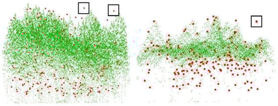
Figure 5.
The point clouds and tree positions of plots 7 and 10. The green points are tree point clouds and the red points are reference tree top positions.
3.5. Tree Height Estimation
In addition to evaluating the detection performance, we also evaluated the correlation between the heights derived from the detected trees and the reference tree heights. The scatter plot of detected heights and reference heights is shown in Figure 6 and the blue line is the fitted line. The R2 reached 0.96. High R2 meant the detected heights were consistent with the reference heights and the trees can be approximately calculated by the detected heights. Because the crown sizes were not provided by the dataset, we cannot estimate the crown sizes. However, the heights and the crown sizes were both predicted by Tree RCNN. Meanwhile, the crown sizes were highly related to the heights. Therefore, if a dataset records the crown sizes of trees, we think the crown sizes can be also well predicted.
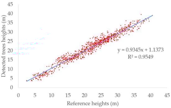
Figure 6.
Scatter plots of detected tree height and reference height. The blue line is the fitted line.
4. Discussion
4.1. Analysis of Model Parameters and Structure
The number of detected trees was affected by the tree probability score threshold and IoUv threshold in the NMS in the second stage. To clearly show the effect of the parameters, the global quantitative estimation results by using tree probability score thresholds (0.3, 0.4, 0.5) and IoUv thresholds (0.2, 0.3, 0.4) are shown in Table 4. As the score threshold increased, the RMSextr, RMSass, and RMScom decreased. This was because if the score threshold was higher, the proposals with higher tree probabilities can remain. As the IoUv Threshold increased, the RMSextr, RMSass, and RMScom increased. This was because if IoUv threshold was higher, the proposals with larger intersections with other proposals can remain. For the combinations of score threshold and IoUv threshold, using score threshold 0.4 and IoUv threshold 0.4 achieved the most satisfactory results, which balanced the RMSextr and RMSass. However, for the other combinations, the RMSextr and RMSass were still relatively satisfactory. The RMSass of most of the Tree RCNN with different thresholds was large than 50% and the RMSextr of most of the Tree RCNN with different thresholds was around 100%. All the results showed our methods can obtain stable accuracy for different parameters.
Table 4.
Detection performance of Tree RCNN with different IoUv thresholds and score thresholds for all plots.
To clearly understand the performance of the proposed dense anchors, utilization of prior knowledge, and multi-position feature extraction for tree detection, the detection performance of three other versions of the Tree RCNN, i.e., Tree RCNN v1, Tree RCNN v2, and Tree RCNN v3, is shown in Table 5. Tree RCNN v1 was the Tree RCNN that only used dense anchors. Tree RCNN v2 was the Tree RCNN that used dense anchors and prior knowledge. Tree RCNN v3 was the Tree RCNN that used dense anchors and multi-position feature extraction. For the Tree RCNN v1, most of the trees were detected and a few misrecognized trees were provided. The RMSass reached 52% and the RMSextr was only 123%. The results demonstrated dense anchors performed well in the forest and fitted the complex forest scenes well. For the Tree RCNN v2, the RMSass increased by adding Al. However, the RMSextr was significantly increased with the RMSass, which induced too many misrecognized trees to be detected. It was mainly because by adding Al, the number of anchors increased. The network detected more trees by the increased anchors, but it did not have enough feature representation ability to discriminate these anchors containing no tree. For the Tree RCNN v3, by adding multi-position feature extraction, the RMSass was higher than the RMSass obtained by Tree RCNN v1. The RMSextr was higher than the RMSextr obtained by Tree RCNN v1 but lower than the RMSextr obtained by Tree RCNN v2. It was mainly because the multi-position feature extraction improved the tree recognition ability but at the same time overfitting occurred to trees. By using all these proposed parts, the Tree RCNN had both better RMSass and RMSextr than Tree RCNN v2 and Tree RCNN v3. Compared to Tree RCNN v1, the RMSass increased, but not greatly. Although using either the utilization of prior knowledge or multi-position feature extraction failed to obtain better results than only using dense anchors, the combination of the two proposed approaches improved the results. This was mainly because the prior knowledge provided extra anchors and the improved feature extraction ability can learn useful features from the extra anchors to improve the detection performance.
Table 5.
Detection performance of Tree RCNN with a different structure for all plots.
4.2. Comparison with Other Methods
To better understand the performance of Tree RCNN, we further compared Tree RCNN with the models provided by NEWFOR [20]. Additionally, the current commonly used object detection deep learning methods such as SECOND [28], PV-RCNN [29], and PointRCNN [30] were used for tree detection to investigate the performance of these methods. The global quantitative estimation results for these methods are shown in Table 6.
Table 6.
Detection performance of different models for all plots.
For the models provided by NEWFOR, i.e., methods 1–8, the RMSass of most methods were lower than 50%, and only methods 5 and 6 had better RMSass which reached 53 and 54, respectively. The results showed most of the methods cannot detect trees well in forests and nearly half of the trees cannot be detected. For the commonly used deep learning methods, although PointRCNN can directly operate on point clouds, almost none of the trees were detected by the method. The main reason for the failure of individual tree detection was that the point-wise features were used to distinguish individual trees in the method. The point-wise features cannot catch the overall shape features of individual trees but only focus on the local point distributions which were very similar in forests. The PV-RCNN and SECOND encoded the point distributions into voxel-based features and extracted features for the voxels by sparse CNNs. As the receptive fields of CNNs became increasingly bigger in the feature extraction process, the overall shape features of individual trees can be caught and the two methods can be used to detect trees in forests. However, since these two methods mainly focused on urban scenes, they showed no advantage over the methods without deep learning in the forests. Thanks to the specific design for forests, compared to all these methods, our method achieves the highest RMSass, which reached 61%. Meanwhile, compared to methods 5, 6, 10, and 11 whose RMSass and RMSextr were lower but close to our method, the RMScom of our method was no larger than those of the methods. Since the method can detect more trees and propose fewer misrecognized trees, it is more suitable than those the other methods for tree detection in forests. For the detected trees, the RMSH and RMSV of the deep learning methods including our method were larger than the other methods. It was because different from the no deep learning methods, the positions of the trees were predicted by the trained deep learning methods. In the training process, the deep learning methods forced the predicted tree positions to be close to the reference tree positions by the optimized functions similar to Equations (3) and (4). However, because of the inaccurate tree number and tree height in the dataset mentioned in Section 3.1, the reference tree positions were not the actual tree positions. Figure 5 shows the examples, in the black boxes where the reference tree positions are far away from any possible tree tops in the point cloud. Inaccurate tree positions in the training process would produce inaccurate tree positions in the prediction process. If the tree positions were more accurate in the dataset, the detection rates and position accuracy of trees obtained by deep learning methods would be further improved.
To highlight the performance of Tree RCNN in understory vegetation, the matching results in different height layers by these methods are shown in Table 7. For the models provided by NEWFOR, the RMSass of most methods for the layers < 20 m was lower than 40%. Even worse, for the layers <10 m, the RMSass of most methods was lower than 10%. Because method 5 can directly operate on point clouds, for the layers < 20 m, the RMSass of the method was higher than those of other methods. However, the RMSass only reached 15 in layers 2–5 m and 17 in layers 5–10 m. The low RMSass showed that these methods cannot detect trees well in the understory vegetation. Thanks to the proposed anchors, Tree RCNN can detect trees anywhere in the forest without being affected by overstory vegetation. As a result, the RMSass of Tree RCNN was much better than those of methods 1–8. For the layers ranging from 5 m to 20 m, the RMSass of Tree RCNN was at least 15% higher than the best RMSass of methods 1–8. The two deep learning methods such as PV-RCNN and SECOND also had better RMSass in lower layers, compared to methods 1–8. It was mainly because the two methods also used their designed anchors which can directly detect small trees. However, because of the fixed voxel sizes and anchor sizes, the two methods can only perform well in parts of the layers which fitted the setting of the voxel sizes and anchor sizes well. In layers 2–5 m and layers > 20 m, the RMSass of PV-RCNN and SECOND became low. Thanks to the high-wise anchors, the Tree RCNN can detect different sizes of trees well. Our method achieved the best performance in all layers < 20 m.
Table 7.
Detection performance of different models for different height layers.
For the uppermost layers, the RMSass of our method was not the best and the deep learning methods had no advantage over the no deep learning methods. The relatively weak performance was still because of the inaccurate tree number and tree height in the dataset. Meanwhile, the higher a tree is, the easier it is for the tree top position to deviate from the tree root position. Therefore, for the uppermost layers, the predicted tree positions would be easily out of the criteria in the candidate search, which induced the detected trees not to match with the reference trees. However, the RMSass of our method was still higher than that of the seven methods and significantly higher than that of the other deep learning methods, which meant our method was still a competitive method for the uppermost layers.
4.3. Analysis of the Structure of Tree RCNN
The small trees were often clumped together and overlapped by large trees. If the small trees were detected from raster images, they would be lost in the raster images. Therefore, the current deep learning method such as [34,35,36,37] cannot detect small trees well. To solve this problem and improve the detection rate, a complete 3D detection process is needed. The Tree RCNN is the network that can detect trees in a 3D process. The method can directly focus on the anchors that can be generated anywhere in the forest. Meanwhile, if the anchors are generated densely enough, all the trees can have large IoUv with the anchors. Furthermore, in the second stage, as only the features extracted from the points in the proposals were used to predict better tree proposals, the points of the large trees outside the proposals would not affect the small trees. Therefore, the Tree RCNN can well detect trees. Meanwhile, we can find Tree RCNN did not require additional segmentation to improve the detection rate and assumption of hierarchical forest structure.
Although using anchors for detection is a 3D detection process, the computation is unaffordable, if using the 3D anchors directly extended from 2D anchors. In the first stage, feature extraction for 3D sliding windows was the most wasteful of computing resources. The fewer sliding windows were needed, the fewer computing resources were needed. If using the 3D anchors directly extended from the 2D anchors, the number of the 3D anchors was the same as that of the 3D sliding windows. To obtain dense anchors, a very small SI was needed, which required a large number of sliding windows, and the computing resources were unaffordable. However, the number of our proposed 3D dense anchors was almost irrelevant to the number of 3D sliding windows but only related to SI. In this way, we can set a small SI and a large SW to generate dense 3D anchors with a few sliding windows. If using the same setting at a height level, compared to our method, about LN times sliding windows were needed by using the directly extended 3D anchors. Therefore, our anchor points significantly reduced the computation.
PointRCNN showed a two-stage method that can generate anchors by point-wise features. Extracting point-wise features was more efficient than the process in which anchors were first generated and then features were extracted from the points in anchors used in our method. However, because all points in the forest are tree points, whether there is a tree or not cannot be determined only by pointwise features, but can only be recognized by the overall point distribution in a 3D box located here. The failure of individual tree detection for PointRCNN proved it. Therefore, 3D anchors were needed for tree detection.
The IoUv of tree proposals and ground truth trees in the second stage were higher than that of sliding windows and ground truth trees in the first stage. Therefore, the tree proposals predicted in the first stage were not very accurate. The second stage was needed to improve the detection performance. However, the first stage cannot be replaced by directly extracting features from anchors because of the large computation. The process was a coarse-to-fine process.
In the anchor setting, since SI was related to the height of the sliding window, 3D sliding windows with different heights can generate different numbers of location indexes and the corresponding Ad, which was more consistent with the distribution of trees in forests. High trees would not get too close and fewer anchors were generated in high sliding windows to reduce computation. Meanwhile, in low sliding windows, anchors were generated denser to avoid missing low trees.
In this paper, because of lacking ground truth crown sizes, both the scale and aspect ratio of the 3D anchor were 1. If there were crown sizes and our method was applied in the mixed forest, the scales and aspect ratios can be set similarly to Faster R-CNN [25] to fit the crown better. Meanwhile, using multiple scales and aspect ratios does not add the number of sliding windows for feature extraction.
4.4. Further Work and Application
Despite satisfactory accuracy, some further improvements can be made for Tree RCNN or tree detection.
- As we can find from the results, the performance of our method was limited by the inaccurate information in the dataset and the insufficient training data. Data is important for deep learning. A large and accurate dataset can facilitate the development of deep learning in tree detection and the application of LiDAR in forests. Meanwhile, compared to NEWFOR dataset, in addition to increasing tree number, tree types, and forest point clouds with different point densities, the suitable tree dataset for deep learning should contain three improvements. First, the tree number and tree heights should be the same in the LiDAR collection data and ground survey data. The LiDAR collection date should be close to the ground inventory date. The trees should be protected from changes in the interval of the LiDAR collection date and ground inventory date. Second, the tree top positions should be collected. Even if the positions cannot be collected very accurately, the approximate positions with small errors were also allowable. Since trees are not perfectly vertical, using both tree top and root positions can help draw the tree shapes better than only using the root positions and tree heights. Third, the crown sizes should be collected. Although in the paper, using a function can approximately calculate the crown sizes of trees, more accurate crown sizes can better determine the scopes of trees. If the crown sizes are larger than the actual sizes, too much around tree points will be contained in the crowns. Meanwhile, if the crown sizes are smaller than the actual sizes, parts of the points will be cut by the crown scopes. Both of the two cases will decrease the tree detection performance.
- If a dataset records both tree top and root positions, using sloping anchors whose top centers are the tree top positions and bottom centers are the tree root positions can fit the trees better than the vertical anchors. The performance of the Tree RCNN would be improved by using such sloping anchors.
- PointNet++ is a much-used method and many more powerful networks have been proposed such as Kernel Point Convolution (KPConv) [45] and transformer networks [46]. These networks would further improve the detection performance but they were not studied in the paper. In this paper, we focused on the architecture of the network which can detect trees in a 3D detection process. Based on the architecture, different feature extraction networks can be configured for the network. In the future, we will try to use these point feature extraction networks for large datasets to further improve the tree detection ability.
In addition to the further improvements, the good detection performance makes tree RCNN a powerful tool in many aspects. First, Tree RCNN can better detect the understory vegetation for high-accuracy tree detection. Compared with the low detection rates of the current methods for understory vegetation, the improvement of the detection rates expands the application of LiDAR in different forest species. Second, as shown in Table 6 and Table 7, the commonly used deep learning methods could not achieve good performance in forest scenes, in which the objects overlapped each other. The proposed dense anchors in Tree RCNN provide a useful reference for point cloud object detection in crowded scenes similar to forests.
5. Conclusions
This paper has presented a two-stage deep learning network, i.e., Tree RCNN, which can directly detect trees in a 3D detection process. In the first stage, the 3D anchors were proposed to generate tree proposals. For the 3D anchors, the dense anchors can be generated anywhere even in the lower layers of forests. The anchors around local maxima points were generated to better propose large trees. The combination of the two anchors ensured as many trees as possible were proposed. Since the proposed 3D anchors were associated with the dense positions in the sliding windows, the computation was affordable, which ensured the Tree RCNN can directly operate on point clouds. In the second stage, the tree proposals were refined by the features extracted by multi-position feature extraction from the points in the proposals. The detected tree positions were obtained from the refined tree proposals. The performance of the Tree RCNN was tested on the NEWFOR dataset. The results showed the Tree RCNN performed well for trees with different tree types and heights and outperformed the methods provided by the NEWFOR dataset and three commonly used deep learning methods. The better performance demonstrated Tree RCNN is a promising method in the detection of trees, especially the understory trees in forests.
Author Contributions
Conceptualization, Z.W. and Z.K.; methodology, Z.W., P.L., Y.C. and S.L.; software, Z.W. and P.L.; validation, Z.W., Y.C. and S.L.; formal analysis, Z.W. and Y.C.; investigation, P.L., Y.C. and S.L.; resources, Z.W. and Z.K.; data curation, Z.W. and P.L.; writing—original draft preparation, Z.W.; writing—review and editing, Z.W. and P.L.; visualization, P.L.; supervision, Z.W.; project administration, Z.W.; funding acquisition, Z.W. All authors have read and agreed to the published version of the manuscript.
Funding
This research was funded by National Natural Science Foundation of China, grant number 41901414.
Data Availability Statement
The data are public datasets at http://www.newfor.net/download-newfor-single-tree-detection-benchmark-dataset, accessed on 12 March 2015.
Conflicts of Interest
The authors declare no conflict of interest.
References
- Zaforemska, A.; Xiao, W.; Gaulton, R. Individual Tree Detection from Uav Lidar Data in a Mixed Species Woodland. In Proceedings of the ISPRS Geospatial Week 2019, Enschede, The Netherlands, 10–14 June 2019. [Google Scholar]
- Brian, M.W.; Martin, W.R.; Boston, K.; Warren, B.C.; Gitelman, A.; Michael, J.O. Prediction of understory vegetation cover with airborne lidar in an interior ponderosapine forest. Remote Sens. Environ. 2012, 124, 730–741. [Google Scholar]
- Jin, Y.; Liu, C.; Qian, S.; Luo, Y.; Zhou, R.; Tang, J.; Bao, W. Large-scale patterns of understory biomass and its allocation across China’s forests. Sci. Total Environ. 2022, 804, 150169. [Google Scholar] [CrossRef]
- Yang, J.; Kang, Z.; Cheng, S.; Yang, Z.; Akwensi, P.H. An Individual Tree Segmentation Method Based on Watershed Algorithm and Three-Dimensional Spatial Distribution Analysis From Airborne LiDAR Point Clouds. IEEE J. Sel. Top. Appl. Earth Observ. Remote Sens. 2020, 13, 1055–1067. [Google Scholar] [CrossRef]
- Harikumar, A.; Bovolo, F.; Bruzzone, L. A local projection-based approach to individual tree detection and 3-D crown delineation in multistoried coniferous forests using high-density airborne lidar data. IEEE Trans. Geosci. Remote Sens. 2019, 57, 1168–1182. [Google Scholar] [CrossRef]
- Weinstein, B.G.; Marconi, S.; Bohlman, S.; Zare, A.; White, E. Individual Tree-Crown Detection in RGB Imagery Using Semi-Supervised Deep Learning Neural Networks. Remote Sens. 2019, 11, 1309. [Google Scholar] [CrossRef]
- Dai, W.; Yang, B.; Dong, Z.; Shaker, A. A new method for 3D individual tree extraction using multispectral airborne LiDAR point clouds. ISPRS-J. Photogramm. Remote Sens. 2018, 144, 400–411. [Google Scholar] [CrossRef]
- Solberg, S.; Næsset, E.; Bollandsås, O.M. Single Tree Segmentation Using Airborne Laser Scanner Data in a Structurally Heterogeneous Spruce Forest. Photogramm. Eng. Remote Sens. 2006, 72, 1369–1378. [Google Scholar] [CrossRef]
- Koch, B.; Heyder, U.; Weinacker, H. Detection of Individual Tree Crowns in Airborne Lidar Data. Photogramm. Eng. Remote Sens. 2006, 72, 357–363. [Google Scholar] [CrossRef]
- Chen, Q.; Baldocchi, D.; Gong, P.; Kelly, M. Isolating individual trees in a savanna woodland using small footprint lidar data. Photogramm. Eng. Remote Sens. 2006, 72, 923–932. [Google Scholar] [CrossRef]
- Brandtberg, T.; Warner, T.A.; Landenberger, R.E.; McGraw, J.B. Detection and analysis of individual leaf-off tree crowns in small footprint, high sampling density lidar data from the eastern deciduous forest in North America. Remote Sens. Environ. 2003, 85, 290–303. [Google Scholar] [CrossRef]
- Paris, C.; Valduga, D.; Bruzzone, L. A hierarchical approach to three-dimensional segmentation of lidar data at single-tree level in a multilayered forest. IEEE Trans. Geosci. Remote Sens. 2016, 54, 4190–4203. [Google Scholar] [CrossRef]
- Lähivaara, T.; Seppänen, A.; Kaipio, J.P.; Vauhkonen, J.; Korhonen, L.; Tokola, T.; Maltamo, M. Bayesian Approach to Tree Detection Based on Airborne Laser Scanning Data. IEEE Trans. Geosci. Remote Sens. 2014, 52, 2690–2699. [Google Scholar] [CrossRef]
- Zhang, J.; Sohn, G.; Brédif, M. A hybrid framework for single tree detection from airborne laser scanning data: A case study in temperate mature coniferous forests in Ontario, Canada. ISPRS-J. Photogramm. Remote Sens. 2014, 98, 44–57. [Google Scholar] [CrossRef]
- Pirotti, F. Assessing a Template Matching Approach for Tree Height and Position Extraction from Lidar-Derived Canopy Height Models of Pinus Pinaster Stands. Forests 2010, 1, 194–208. [Google Scholar] [CrossRef]
- Mongus, D.; Žalik, B. An efficient approach to 3D single tree-crown delineation in LiDAR data. ISPRS-J. Photogramm. Remote Sens. 2015, 108, 219–233. [Google Scholar] [CrossRef]
- Ferraz, A.; Bretar, F.; Jacquemoud, S.; Gonçalves, G.; Pereira, L.; Tomé, M.; Soares, P. 3-D mapping of a multi-layered Mediterranean forest using ALS data. Remote Sens. Environ. 2015, 121, 210–223. [Google Scholar] [CrossRef]
- Reitberger, J.; Schnörr, C.; Krzystek, P.; Stilla, U. 3D segmentation of single trees exploiting full waveform LIDAR data. ISPRS-J. Photogramm. Remote Sens. 2019, 64, 561–574. [Google Scholar] [CrossRef]
- Gupta, S.; Weinacker, H.; Koch, B. Comparative Analysis of Clustering-Based Approaches for 3-D Single Tree Detection Using Airborne Fullwave Lidar Data. Remote Sens. 2010, 2, 968–989. [Google Scholar] [CrossRef]
- Eysn, L.; Hollaus, M.; Lindberg, E.; Berger, F.; Monnet, J.M.; Dalponte, M.; Kobal, M.; Pellegrini, M.; Lingua, E.; Mongus, D.; et al. A Benchmark of Lidar-Based Single Tree Detection Methods Using Heterogeneous Forest Data from the Alpine Space. Forests 2015, 6, 1721–1747. [Google Scholar] [CrossRef]
- Hao, Y.; Widagdo, F.R.A.; Liu, X.; Liu, Y.; Dong, L.; Li, F. A Hierarchical Region-Merging Algorithm for 3-D Segmentation of Individual Trees Using UAV-LiDAR Point Clouds. IEEE Trans. Geosci. Remote Sens. 2022, 60, 1–12. [Google Scholar] [CrossRef]
- Williams, J.; Schönlieb, C.-B.; Swinfield, T.; Lee, J.; Cai, X.; Qie, L.; David, A.C. 3D Segmentation of Trees through a Flexible Multiclass Graph Cut Algorithm. IEEE Trans. Geosci. Remote Sens. 2020, 58, 754–776. [Google Scholar] [CrossRef]
- Hamraz, H.; Contreras, M.A.; Zhang, J. Vertical stratification of forest canopy for segmentation of understory trees within small-footprint airborne LiDAR point clouds. ISPRS J. Photogramm. Remote Sens. 2017, 130, 385–392. [Google Scholar] [CrossRef]
- Hamraz, H.; Contreras, M.A.; Zhang, J. A robust approach for tree segmentation in deciduous forests using small-footprint airborne LiDAR data. Int. J. Appl. Earth Obs. Geoinf. 2016, 52, 532–541. [Google Scholar] [CrossRef]
- Ren, S.; He, K.; Girshick, R.; Sun, J. Faster R-CNN: Towards Real-Time Object Detection with Region Proposal Networks. IEEE Trans. Pattern Anal. Mach. Intell. 2017, 39, 1137–1149. [Google Scholar] [CrossRef] [PubMed]
- Bochkovskiy, A. YOLOv4: Optimal Speed and Accuracy of Object Detection. arXiv 2020, arXiv:2004.10934. [Google Scholar]
- Lin, T.Y.; Goyal, P.; Girshick, R.; He, K.; Dollár, P. Focal Loss for Dense Object Detection. arXiv 2017, arXiv:1708.02002. [Google Scholar]
- Yan, Y.; Mao, Y.; Li, B. SECOND: Sparsely Embedded Convolutional Detection. Sensors 2018, 18, 3337. [Google Scholar] [CrossRef]
- Shi, S.; Guo, C.; Jiang, L.; Wang, Z.; Shi, J.; Wang, X.; Li, H. PV-RCNN: Point-Voxel Feature Set Abstraction for 3D Object Detection. arXiv 2019, arXiv:1912.13192. [Google Scholar]
- Shi, S.; Wang, X.; Li, H. PointR-CNN: 3D Object Proposal Generation and Detection From Point Cloud. In Proceedings of the IEEE/CVF Conference on Computer Vision and Pattern Recognition (CVPR), Long Beach, CA, USA, 15–20 June 2019. [Google Scholar]
- Zhu, Y.; Zhou, J.; Yang, Y.; Liu, L.; Liu, F.; Kong, W. Rapid Target Detection of Fruit Trees Using UAV Imaging and Improved Light YOLOv4 Algorithm. Remote Sens. 2022, 14, 4324. [Google Scholar] [CrossRef]
- Ocer, N.E.; Kaplan, G.; Erdem, F.; Kucuk Matci, D.; Avdan, U. Tree extraction from multi-scale UAV images using Mask R-CNN with FPN. Remote Sens. Lett. 2020, 11, 847–856. [Google Scholar] [CrossRef]
- Zamboni, P.; Junior, J.; Silva, J.; Miyoshi, G.; MAtsubara, E.; Nogueira, K.; Goncalves, W. Benchmarking Anchor-Based and Anchor-Free State-of-the-Art Deep Learning Methods for Individual Tree Detection in RGB High-Resolution Images. Remote Sens. 2021, 13, 2482. [Google Scholar] [CrossRef]
- Windrim, L.; Bryson, M. Detection, Segmentation, and Model Fitting of Individual Tree Stems from Airborne Laser Scanning of Forests Using Deep Learning. Remote Sens. 2020, 12, 1469. [Google Scholar] [CrossRef]
- Li, Y.; Chai, G.; Wang, Y.; Lei, L.; Zhang, X. ACE R-CNN: An Attention Complementary and Edge Detection-Based Instance Segmentation Algorithm for Individual Tree Species Identification Using UAV RGB Images and LiDAR Data. Remote Sens. 2022, 14, 3035. [Google Scholar] [CrossRef]
- Schmohl, S.; Vallejo, A.; Soergel, U. Individual Tree Detection in Urban ALS Point Clouds with 3D Convolutional Networks. Remote Sens. 2022, 14, 1317. [Google Scholar] [CrossRef]
- Luo, Z.; Zhang, Z.; Li, W.; Chen, Y.; Wang, C.; Nurunnabi, A.; Li, J. Detection of Individual Trees in UAV LiDAR Point Clouds Using a Deep Learning Framework Based on Multichannel Representation. IEEE Trans. Geosci. Remote. Sens. 2022, 60, 1–15. [Google Scholar] [CrossRef]
- NEWFOR. The NEWFOR Single Tree Detection Benchmark Dataset. Available online: http://www.newfor.net/download-newfor-single-tree-detection-benchmark-dataset (accessed on 1 February 2015).
- Su, H.; Maji, S.; Kalogerakis, E.; Learned-Miller, E. Multi-view Convolutional Neural Networks for 3D Shape Recognition. In Proceedings of the IEEE International Conference on Computer Vision (ICCV), Santiago, Chile, 7–13 December 2015. [Google Scholar]
- Amiri, N.; Polewski, P.; Yao, W.; Krzystek, P.; Skidmore, A.K. Detection of Single Tree Stems in Forested Areas from High Density Als Point Clouds Using 3d Shape Descriptors. In Proceedings of the ISPRS Geospatial Week 2017, Wuhan, China, 18–22 September 2017. [Google Scholar]
- Curtis, R.O.; Reukema, D.L. Crown Development and Site Estimates in a Douglas-Fir Plantation Spacing Test. For. Sci. 1970, 16, 287–301. [Google Scholar]
- Qi, C.R.; Yi, L.; Su, H.; Guibas, L.J. PointNet++: Deep Hierarchical Feature Learning on Point Sets in a Metric Space. arXiv 2017, arXiv:1706.02413. [Google Scholar]
- Girshick, R. Fast R-CNN. In Proceedings of the 2015 IEEE International Conference on Computer Vision (ICCV), Santiago, Chile, 7–13 December 2015. [Google Scholar]
- Duchi, J.; Hazan, E.; Singer, Y. Adaptive subgradient methods for online learning and stochastic optimization. J. Mach. Learn. Res. 2011, 12, 257–259. [Google Scholar]
- Thomas, H.; Qi, C.R.; Deschaud, J.E.; Marcotegui, B.; Goulette, F.; Guibas, L. KPConv: Flexible and Deformable Convolution for Point Clouds. In Proceedings of the 2015 IEEE International Conference on Computer Vision (ICCV), Seoul, Republic of Korea, 27 October–2 November 2019. [Google Scholar]
- Vaswani, A.; Shazeer, N.; Parmar, N.; Uszkoreit, J.; Jones, L.; Gomez, A.N.; Kaiser, L.; Polosukhin, I. Attention Is All You Need. arXiv 2017, arXiv:1706.03762. [Google Scholar]

Disclaimer/Publisher’s Note: The statements, opinions and data contained in all publications are solely those of the individual author(s) and contributor(s) and not of MDPI and/or the editor(s). MDPI and/or the editor(s) disclaim responsibility for any injury to people or property resulting from any ideas, methods, instructions or products referred to in the content. |
© 2023 by the authors. Licensee MDPI, Basel, Switzerland. This article is an open access article distributed under the terms and conditions of the Creative Commons Attribution (CC BY) license (https://creativecommons.org/licenses/by/4.0/).