Article

Early Yield Forecasting of Maize by Combining Remote Sensing Images and Field Data with Logistic Models

1
State Key Laboratory of Simulation and Regulation of Water Cycle in River Basin, China Institute of Water Resources and Hydropower Research, Beijing 100038, China
2
National Center for Efficient Irrigation Engineering and Technology Research-Beijing, Beijing 100048, China
*
Author to whom correspondence should be addressed.
Remote Sens. 2023, 15(4), 1025; https://doi.org/10.3390/rs15041025
Submission received: 9 January 2023 / Revised: 10 February 2023 / Accepted: 10 February 2023 / Published: 13 February 2023
(This article belongs to the Special Issue Crops and Vegetation Monitoring with Remote/Proximal Sensing)

Abstract

:
Early forecasting of crop yield from field to region is important for stabilizing markets and safeguarding food security. Producing a precise forecasting result with fewer inputs is an ongoing goal for the large-area yield evaluation. We present one approach of yield prediction for maize that was explored by incorporating remote-sensing-derived land surface temperature (LST) and field in-season data into a series of logistic models with only a few parameters. Continuous observation data of maize were utilized to calibrate and validate the corresponding logistic models for regional biomass estimating based on field temperatures (including crop canopy temperature (Tc)) and relative dry/fresh biomass accumulation. The LST maps from MOD11A1 products, which are considered to be matched as Tc in large irrigation districts, were assimilated into the validated models to estimate the biomass accumulation. It was found that the temporal-scale difference between the instantaneous LST and the daily average value of field-measured Tc was eliminated by data normalization method, indicating that the normalized LST could be input directly into the model as an approximation of the normalized Tc. Making one observed biomass in-season as the driving force, the maximum of dry/fresh biomass accumulation (DBA/FBA) at harvest could be estimated. Then, grain yield forecasting could be achieved according to the local harvest index of maize. Silage and grain yields were evaluated reasonably well compared with field observations based on the regional map of LST values obtained in 2017 in Changchun, Jilin Province, China. Here, satisfactory grain and silage yield forecasting was provided by assimilating once measured value of DBA/FBA at the middle growth period (early August) into the model in advance of harvest. Meanwhile, good results were obtained in the application of this approach using field data in 2016 to predict grain yield ahead of harvest in the Jiefangzha sub-irrigation district, Inner Mongolia, China. This study demonstrated that maize yield can be forecasted accurately prior to harvest by assimilating remote-sensing-derived LST and field data into the logistic models at a regional scale considering the spatio-temporal scale extension of ground information and crop dynamic growth in real time.

1. Introduction

Early estimates of crop yield will contribute to addressing the key issues of crop production management, future market output, and deep processing. According to the early prediction of crop yield, farmers can adjust and optimize irrigation decision making in a timely way to maximize yield for enhancing profits, while policymakers also take reasonable measures to deal with potential trade risks in order to safeguard food security and ensure market stability [1]. It should be emphasized that the earlier yield forecasting information is provided, the more effective measures are likely to be undertaken [2].
Plentiful studies have been implemented to predict final yield in the past decades based on different methods including field survey, statistical methods, and crop growth models [3,4,5]. Field survey can assess yield by capturing the ground truth; nonetheless, it is highly time-consuming and labor-intensive. The core of statistical methods lies in the acquisition of empirical relationships between crop yields and specific related indicators. Despite reasonably accurate results in specific field areas, it is restricted when scaling up this relationship to large areas. Crop growth models can be applied to describe plant dynamic growth. Biomass is a critical biophysical indicator with a close link to yield at harvest. Therefore, one way to predict yield is to acquire biomass estimates via crop growth models and then implement the in-season evaluations of yield on account of their good correlations. Crop growth models include process-based models and experiment regression ones [6]. The former requires many parameters as inputs [7,8], making it difficult to execute the models in data-scarce regions [9] though it is more mechanistic than the latter. In contrast, with only a few parameters, statistical regression models have been developed (e.g., the Richards, Compertz, and Weibull equations) and continue to be widely used to illustrate crop growth dynamics including biomass [10,11,12], but this method has the limitation of extending model parameters to large areas.
Given that these methods have limitations, data assimilation has been developed to solve these problems in yield forecasting. Intrinsically, data assimilation is used to incorporate observations into the model to obtain the optimal possible estimates [13]. The rapid advancement of satellite images allows for large-scale crop growth monitoring [14,15]. Numerous studies have shown that incorporating remote sensing data into crop models can improve regional yield estimates [16,17,18]. The research has focused mainly on the assimilation of mechanism models [2,19,20,21] despite the fact that they require numerous input parameters. By contrast, it is worth investigating the potential of experiment regression models in early-season yield forecasting for large areas via data assimilation when there is a lack of detailed input information.
As one of the most important crops, maize yield forecasting is critical for the development of agriculture and livestock [22] and can serve as an excellent reference for other crop research. For different purposes, farmers can harvest maize as silage or grain yield, and correspondingly, dry biomass accumulation (DBA) and fresh biomass accumulation (FBA) need to be predicted as an important precondition for yield forecasting.
The logistic model is one of the most commonly applied regression models for crop growth processes such as DBA throughout the growing season [23,24,25,26,27]. However, the logistic model fails to fully describe the development process of FBA or leaf area index (LAI) due to the existence of a downtrend process after the milk stage caused by leaf senescence. A revised logistic model proposed by Wang [28] overcame this limitation and performed well when describing LAI changes [29], but it has not yet been used for FBA. In addition, the logistic model was originally developed for individual plants that neglected regional applicability. Elings [30] acquired maize leaf area dynamic growth in various environments using a set of parameters for the data normalization method. This method has been used to establish a normalized logistic model of relative DBA (RDBA) for simulating regional crop growth patterns [4,31].
Indeed, another major obstacle to the application of the logistic model in region is the choice of input parameter, which serves as a vital bridge linking the point-based and regional applications. Furthermore, previous studies have demonstrated the growth curve of maize using the logistic models with air or soil temperatures as input [32,33,34]. The cropping environment is the most influential factor in plant yield [35,36]. Canopy temperature (Tc) is obviously a better indicator for reflecting crop water message responses to field conditions. Moreover, Tc can be considered as matched to land surface temperature (LST) in large agricultural areas, which can be inversed from remote sensing images [37]. Therefore, integrating LST data into the normalized logistic models can acquire the values of RDBA in combination with the once-measured DBA on a certain date and harvest index (HI), which presents an opportunity to achieve early yield forecasting in regions.
Therefore, an approach was developed to retrieve early prediction of maize yield using logistic models in combination with daily LST images and in-season field observations. The major objectives are as follows: (1) to calibrate and validate the corresponding logistic models for simulating the maize growth curves including RDBA and relative FBA (RFBA) based on different independent variables including temperatures of air, canopy, and soil at 20 cm or 40 cm in the root zone; (2) to determine the applicability of Tc in crop monitoring as well as the appropriate model parameters; (3) to forecast maize yield in region by HI and biomass maximum including DBA and FBA, which can be acquired by incorporating the normalized LST from remote sensing as an approximation of the normalized Tc into the corresponding optimal models with once-observed DBA or FBA as the driving force; and (4) to test the portability of this approach by producing grain yield maps in other agricultural districts and comparing them to local observations.

2. Materials and Methodology
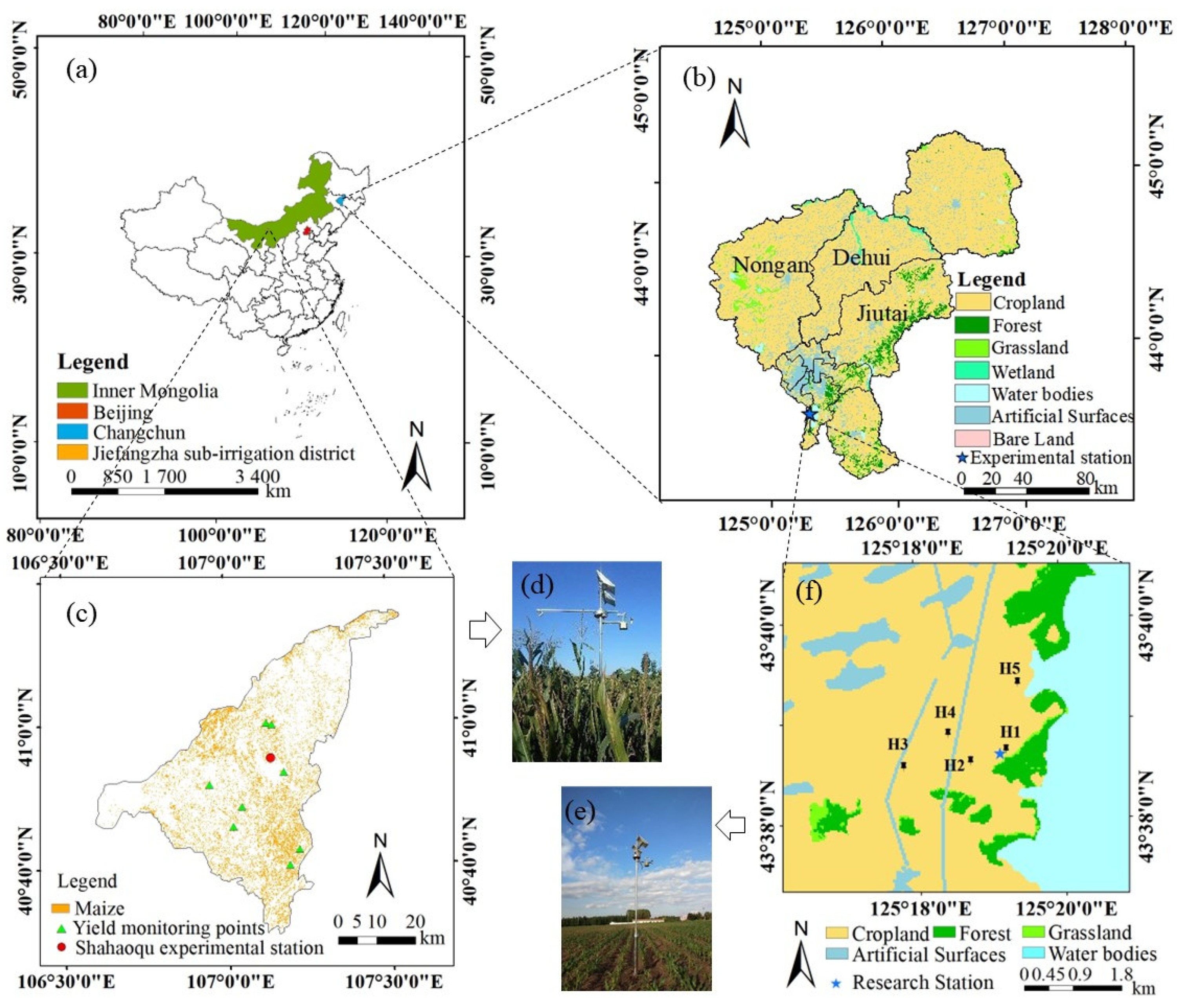
2.1. Study Areas

The first study region was in Changchun area, Jilin Province (about 2.05 million ha), as shown in Figure 1a,b. This region was characterized by a northern temperate continental monsoon climate, with an average annual rainfall of 520–755 mm [38], of which more than 60% occurs in the summer. The annual average daily temperature is 4.8 °C, and the sunshine duration is approximately 2700 h. The data for model developments were obtained from field experiments of maize growth (May–September) from 2017 to 2019 in an agricultural research station (43°38′39.92″N, 125°19′7.77″E, 248 m a.s.l.) near Changchun city, as shown in Figure 1f (about 73 ha). The maize cultivar was Xianyu 335. The predominant soil types are black and meadow soil, and the soil texture is mainly sandy loam soil. The field capacity (Fc) and wilting point (Wp) were measured as 37% and 16% in an 80 cm average of the crop root zone, respectively. Precipitation and soil water content in 2017–2019 were monitored, revealing an optimal soil moisture range for maize growth (Figure 2).
Another study region for this work was the Jiefangzha sub-irrigation district (approximately 0.229 million ha), which is one main component of Hetao irrigation district in Inner Mongolia, China (Figure 1a,c). Maize is one of the major crops in this region. The yearly average daily temperature is 9 °C, with an annual rainfall of approximately 151.3 mm. The field monitoring system was conducted in the Shahaoqu experimental station in 2016, as shown in Figure 1b (40°55′8″N, 107°8′16″E, 1036 m a.s.l.). The values of Fc and Wp are 35% and 15% in the crop root zone, respectively. More information can be found in the report by Bai et al. [39].

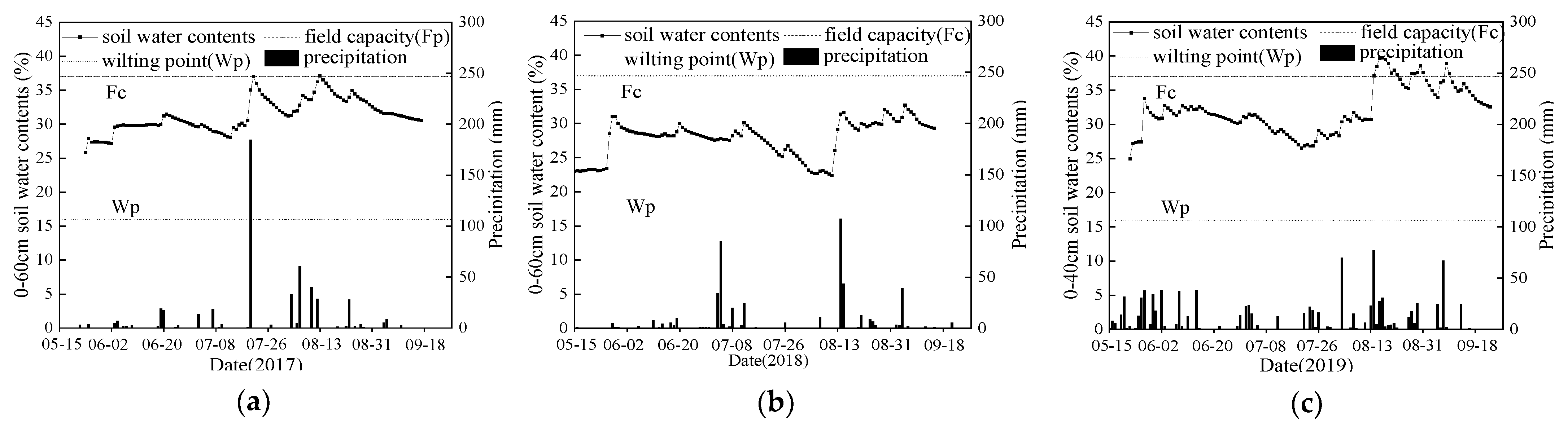
2.2. Field Measurements

In Changchun, the five typical maize plots (named H1 to H5, Figure 1f) were equipped with five sets of canopy temperature and meteorology monitoring systems (CTMS) (Figure 1e), which are composed of a stainless-steel stand column, solar panels, and various sensors. This system can synchronously monitor field data at 30 min intervals, including wind speed (014MINI-MetOne, Washington, USA), solar radiation (SP110-Apogee/SQ110-Apogee, Logan, USA), the crop canopy temperature (TPiS 1 T 1252B, Excelitas, Waltham, Germany), air temperature/humidity (HMP60-Vaisala, Vantaa, Finland), soil temperature/moisture (20 cm and 40 cm in the root zone) (SM10D, Beijing, China), and more by the corresponding sensors. It should be emphasized that the canopy temperature at 30 min intervals was computed as the average of multi-point values around the equipment by the rotation measurement of a thermal infrared sensor (TPiS 1 T 1252B, Excelitas, Waltham, Germany) installed at the end of a cantilever perpendicular to the stand column. Sensors were set up at a height of 3 m during the whole growth stage, which could be adjusted as need. Regular weekly maintenance ensured the normal functioning of the equipment. A more detailed description of the system was provided by Cai et al. [37] and Huang et al. [40].
Above-ground biomass was sampled every 10–15 days by removing three representative plants from each of monitoring plots. The collected samples were immediately weighted as the amount of FBA. Then, these samples were put in an oven at 105 °C for 30 min to stop the plant life activities and subsequently were dried at 80 °C to a constant weight. (The final weight would be the DBA.) During the harvest, the last sampling of above-ground biomass was recorded, and the grain yield (1 m2) and planting density were measured in each experimental point at the same time. In conclusion, six samples were collected from each plot per year.
Similarly, a CTMS system was installed in the Shahaoqu experimental station to collect the same data as Changchun, and eight yield monitoring points were erected to measure final grain yield for evaluation in the Jiefangzha sub-irrigation district (Figure 1c). Furthermore, above-ground biomass in the experimental site was sampled and recorded four times as a driving force for yield forecasting. More details can be seen in the report from Bai et al. [39].

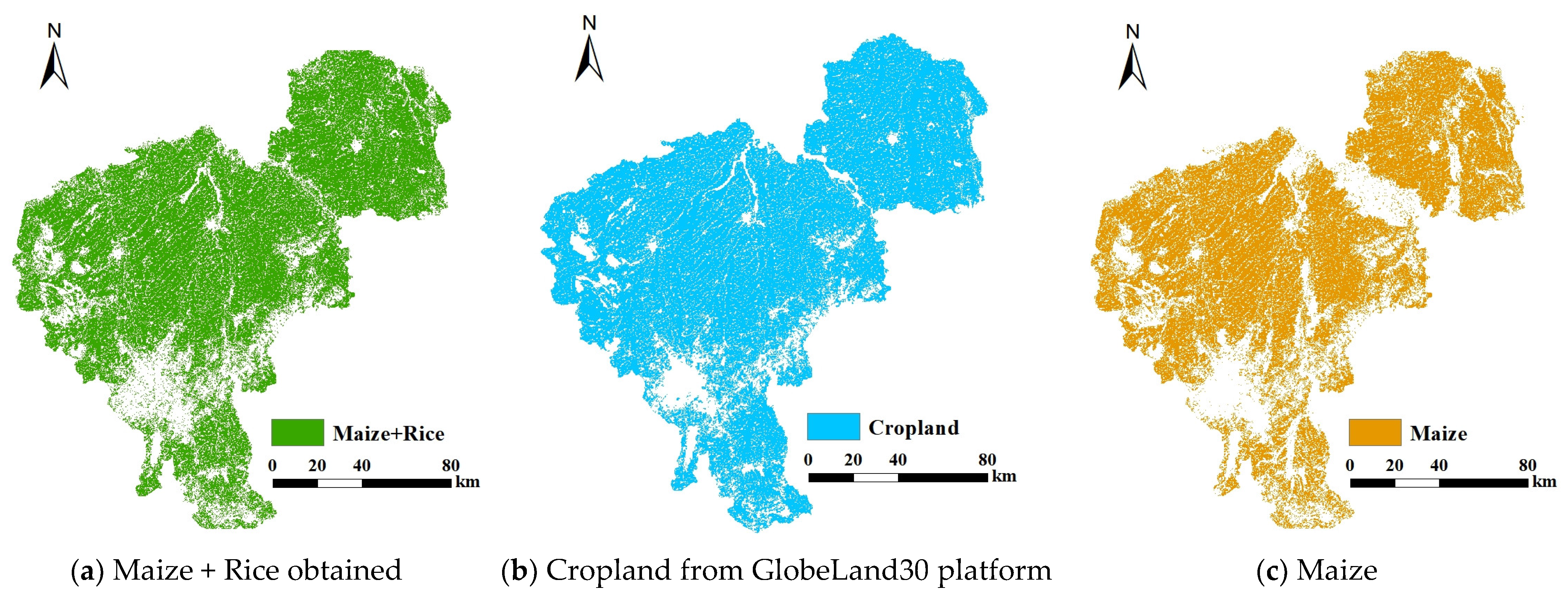
2.3. Remote Sensing Data

For the subsequent spatial-scale research in Changchun, the Landsat 8 images (30 m) and MOD11A1 data (1 km) in 2017 were downloaded from the website of USGS (https://earthexplorer.usgs.gov/ accessed on 21 June 2021) with the aim of acquiring the LST data. The available remote sensing images can be seen in Table S1. Daily LST data were derived from the MOD11A1 product (1 km). Due to the cloudiness, there were only four clear Landsat 8 images in 2017 relevant to maize growth that would be used for mapping maize in the research area and verified by the field monitoring data, cropland map from the GlobeLand30 platform, and statistics data.
To obtain the maize distribution in Changchun, some calculations and preprocessing needed to be finished. Firstly, the normalized difference vegetation index (NDVI) and land surface water index (LSWI) were calculated by Equations (1) and (2), which were also followed for four Landsat 8 images (Operational Land Imager, OLI) [41,42]. The Landsat 8 image on 25 September, which is the best one just in the maize growth stage, was chosen as a sample to classify the region of interest (ROI). The classification thresholds could be determined by combining the features of vegetation in different stages and the changes in NDVI and LSWI of ROI samples. The process contained the following four steps (Figure S1): (1) to distinguish the vegetation and the others according to the NDVI values on 25 September (Julian day 268), which belonged to the optimum discrimination period of vegetation in four images; (2) to obtain the thresholds by analyzing the NDVI values of forest and crop samples on 5 June (Julian day 156), when the crops were in the early growth stage, and the NDVI of the forest should be obviously higher; (3) to employ the LSWI of rice samples in ROI on 5 June (Julian day 156) to determine the corresponding thresholds considering the rice was irrigated during this stage, and the LSWI values of rice should be higher; and (4) to determine the relative thresholds between the maize and the other vegetations by analyzing the LSWI ranges of them in ROI on 5 June (Julian day 156) and 25 September (Julian day 268). Based on these thresholds, the distribution of maize + rice could be obtained according to the classification rules of decision tree classification.
NDVI = ƿ N I R ƿ R E D / ƿ N I R + ƿ R E D
LSWI = ƿ N I R ƿ S W I R / ƿ N I R + ƿ S W I R
where ƿ N I R (band5), ƿ R E D (band4), and ƿ S W I R (band6) are the reflectivity of near-infrared, red, and shortwave infrared band, respectively.
Based on the decision tree classification mentioned above, the combination pattern for maize + rice in Changchun was obtained (Figure 3a). As the dominant field crops are maize and rice here, it was assumed that these results are mostly cropland. In order to evaluate the classification precision, the land-cover data with a spatial resolution of 30 m in 2020 (Figure 3b) were downloaded from the platform of GlobeLand30 (http://www.globallandcover.com/home.html accessed on 3 October 2021), published by the Ministry of Natural Resources of China. Meanwhile, the statistical data of crop areas were obtained from the Statistic Bureau of Jilin Province (http://tjj.jl.gov.cn/tjsj/ accessed on 3 October 2021) for further evaluating the classification precision.
Using the confusion matrix, the value of the producer’s accuracy (ratio of the number of estimated correct pixels to reference pixels) about cropland was 82.18%, determined through comparing Figure 3a,b. This value proved that the classification method established above was available and appropriate. It should be emphasized that the validation method used here was restricted by the accuracy of the GlobeLand30 product. Meanwhile, this product is not offered for every year, which will affect the accuracy evaluation of crop mapping. The maize mapping could be obtained by the same method (Figure 3c), which took up 87% of cropland in Figure 3b. The ratio was consistent with the value from statistics data (84%).
For the Jiefangzha sub-irrigation district, the spatial distribution of maize was derived from the report from Bai et al. [39], as shown in Figure 1c. Fortunately, the images from Landsat 8 (30 m) and MOD11A1 (1 km) can support the enhanced spatial and temporal adaptive reflectance fusion model (ESTARFM) algorithm [43] to improve the spatial accuracy of LST. Therefore, the fused LST was used in this region. Details of the extraction process can be found in research by Huang et al. [40].

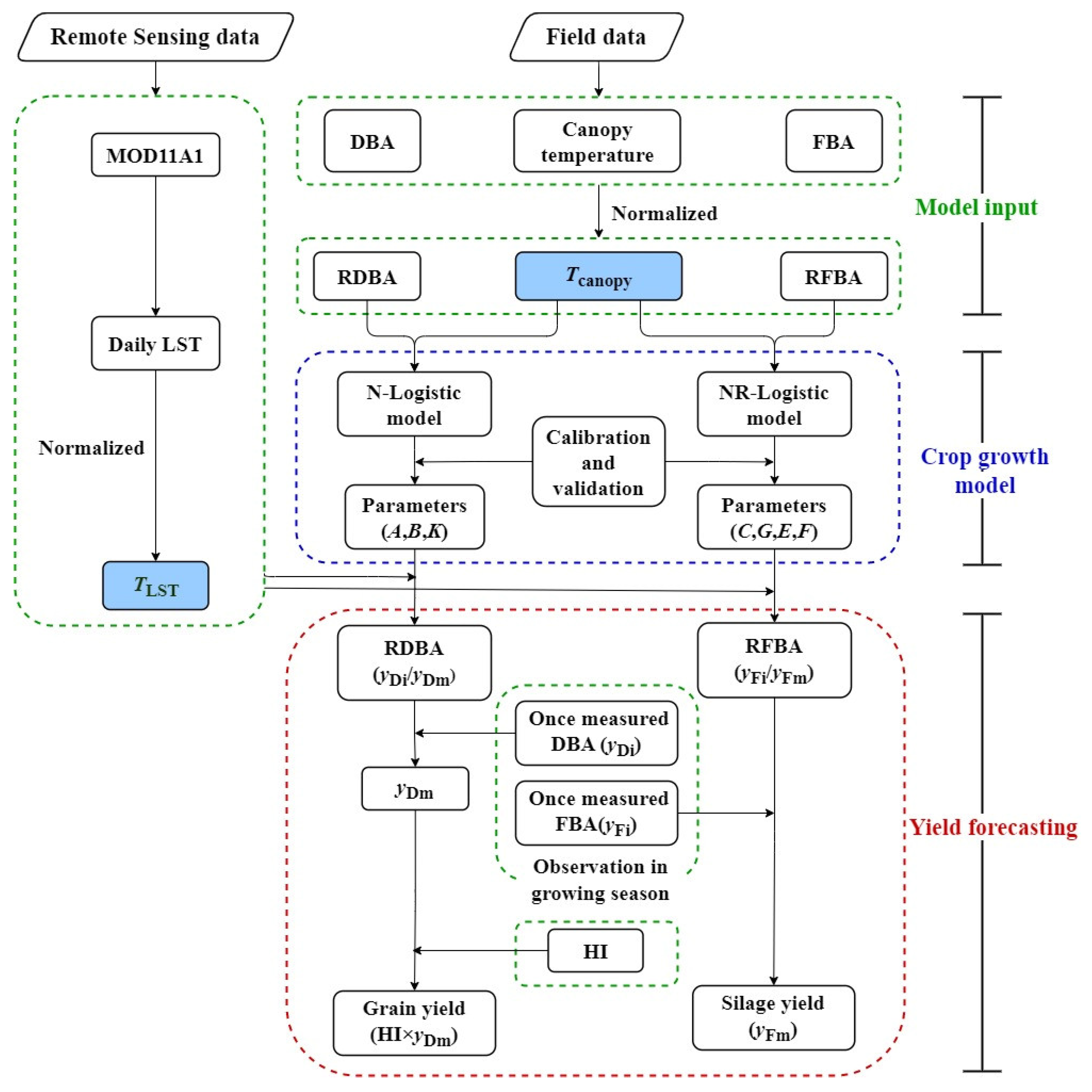
2.4. Logistic Models

2.4.1. Logistic Model

The logistic model depicts a sigmoidal curve [44] that increases gradually at first, more rapidly in the middle, and then slowly at the end before leveling off at a maximum value [45,46], such as the growth curve of DBA [47]. The model equation is as follows:
y D = a / 1 + b exp k t   t = i = 1 n t i 10
where y D is the dependent growth parameter (DBA, kg ha−1); a denotes the uppermost asymptote, implying the theoretical upper limit of DBA growth; b and k are model parameters; t is the effective accumulated temperature after emergence in the present study (hereinafter referred to as the effective accumulated temperature, °C). Notably, tair, tcanopy, t20, and t40 (°C), represent the effective accumulated temperature of the air, canopy, and soil at 20 cm or 40 cm of the root zone, respectively. t i is the day i value (from crop emergence) of daily average temperature of the air, canopy, or soil at 20 cm or 40 cm depth of the crop root zone. (It is calculated as 30 °C when t i exceeds 30 °C, and it will be calculated as 10 °C if the value is less than 10 °C [48].) n is the total number of days from crop emergence to harvest.

2.4.2. Normalized Logistic Model (N-Logistic Model)

The logistic model was originally developed for individual applications that may be inappropriate for spatial prediction of crop growth. The normalization method transforms the raw data into an interval of 0 to 1, which can eliminate the dimensional differences between plots. Therefore, the RDBA and relative effective accumulated temperature (T) were used to set up the growth model, lower data dispersion (from different plots), and form a regional model. Here, the logistic model with normalization is called N-logistic model, which has the same form as the logistic model but with different parameters:
Y D = A / 1 + B exp K T   Y D = y D / y Dm   T = t / t m
where YD is the RDBA, which is the ratio of y D (DBA in the maize growing season) to y Dm (DBA at harvest); A is the upper most asymptote implying the upper limit of RDBA; and B and K are model parameters; t is the same as in Equation (3); t m is equal to the value of t at harvest; T is relative effective accumulative temperature (T20, T40, Tcanopy, and Tair mean the values in soil at 20 cm and 40 cm under surface, crop canopy, and air, respectively), which is the ratio of t to t m . Theoretically, the value of Y D equals A when T (0 ≤ T ≤ 1) reaches 1. Therefore, the value of A represents the theoretical upper limit of the RDBA.

2.4.3. Revised Logistic Model (R-Logistic Model)

Like the simulation of LAI, the R-logistic model [28] was employed to verify the FBA growth pattern:
y F = c / 1 + exp g t 2 + e t + f
where y F is the above-ground FBA (kg ha−1); c, g (>0), e, and f are the model parameters; t is the same as in Equation (3). When t = 0, y F = c / 1 + exp f (the above-ground FBA in maize emergence); when t = (−e/2g), the value of ( g t 2 + e t + f ) reaches a minimum, and the value of y F reaches a maximum; when t > (−e/2g), the value of y F begins to decline. These situations are consistent with the actual growth curve of FBA.

2.4.4. Normalized Revised Logistic Model (NR-Logistic Model)

Similar to the logistic model, the R-logistic model was initially developed for individual plants. To scale up the simulation from a single plot to a region, the NR-logistic model was developed by the normalization method mentioned above. It takes the same form as the R-logistic model but with key parameters:
Y F = C / 1 + exp G T 2 + E T + F   Y F = y F / y Fm
where Y F represents the relative fresh biomass accumulation (RFBA); C, G (>0), E, and F are parameters; T (0 ≤ T ≤ 1) is the same as in Equation (4); y Fm represents the maximum FBA (g m−2). When T = (−E/2G), the value of G T 2 + E T + F reaches a minimum, and Y F reaches a maximum; when (−E/2G) < T < 1, the value of Y F declines as the value of T increases.

2.5. Yield Forecasting

When the model was validated to obtain suitable parameters, namely the RDBA and y Dm , the RFBA and y Fm could be simulated by Equations (4) and (6) with field monitoring data once at least, respectively, when combined with the map of the independent variable (LST) inversed from remote sensing images. Grain yield (Y) will be forecasted by the DBA in harvest period and HI as follows:
Y = HI × y Dm
where Y is grain yield; HI is the weight of a harvested product as a percentage of the total plant weight of a crop; and y Dm is the DBA at harvest time as mentioned above. The values of maize HI in some subareas in Changchun [49] and the measured ones in the experimental station (Table S2) were used to obtain the HI map (Figure S2) in Changchun by the kriging interpolation method.
A flow chart of this approach using canopy temperature to forecast yield is shown in Figure 4. Firstly, the logistic model/R-logistic model was used to prove the possibility to simulate DBA/FBA based on Tc. Secondly, the logistic model/R-Logistic model was changed to N-logistic model/NR-logistic model by the data normalization method for regional biomass (RDBA/RFBA) estimation. Finally, the grain/silage yield can be forecasted using remote-sensing-derived LST and once-measured biomass (DBA/FBA) as inputs to the N-logistic model/NR-logistic model after obtaining the HI value. In Section 3, the grain/silage yield in Changchun would be forecasted using measured DBA on three dates (7/16, 8/10, and 8/31 in 2017), and the grain yield in Jiefangzha would be forecasted by once-measured DBA on four dates (7/6, 7/21, 8/4, and 8/26 in 2016). The independent variable for the N-logistic model and NR-logistic model, i.e., Tcanopy, was a scale factor for yield forecasting from point to area through the LST map from remote sensing images (TLST) in a large irrigation district.

2.6. Statistical Evaluation

The index of model agreement (d), root mean square error (RMSE), relative error (RE), the coefficient of determination (R2), and the coefficient of variation (CV) were used to evaluate the models. Model accuracy increased as the values of d and R2 approached 1.0, and the values of RMSE and RE decreased. Origin Pro 9.1 software was used to calculate and fit the data to the model. Statistical analyses were performed in Microsoft Excel 2013. The calculation formulas are listed in Equations (S1)–(S5).

3. Results

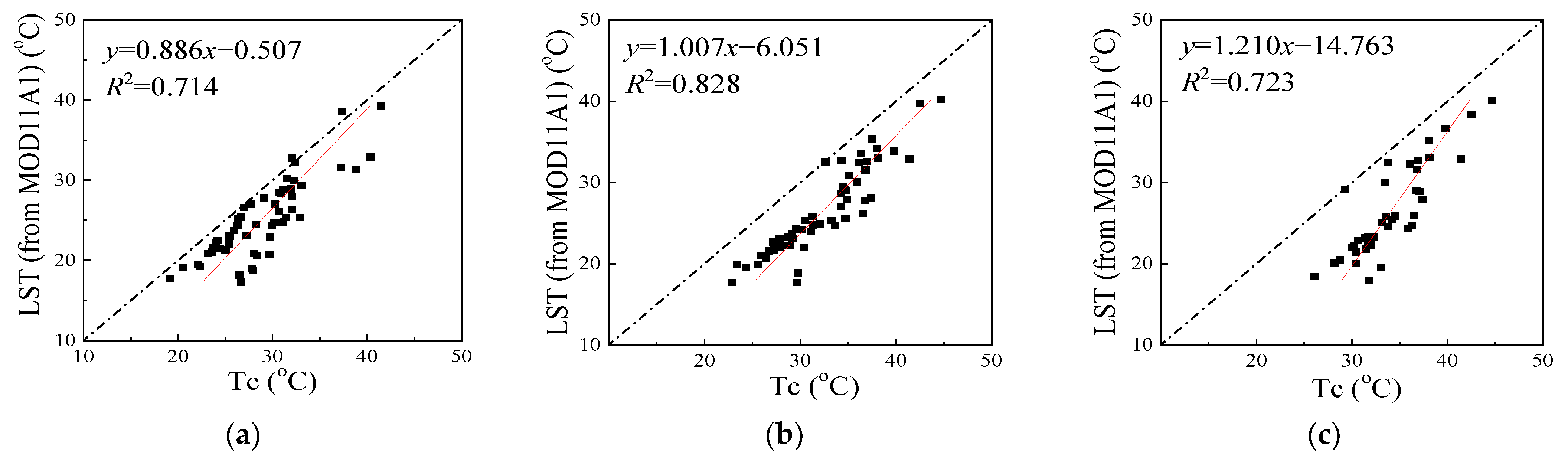
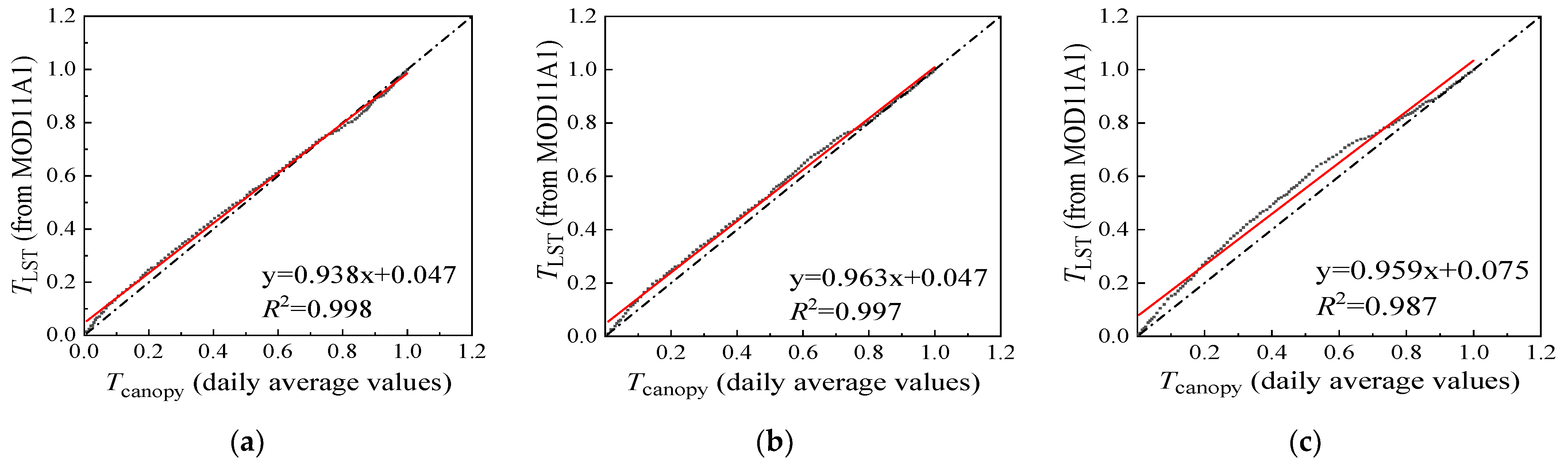
3.1. Evaluating the Values of LST from MOD11A in Changchun

The regional map of LST can be obtained by remote sensing images products—MOD11A1. Afterwards, the grain yield in an area might be estimated through the validated model and retrieval values. Due to cloud cover, there were some incomplete data in MOD11A1 images from 25 May to 21 September 2017. The kriging interpolation method was used to fill the gaps in data.
It is necessary to obtain high-quality input data for precise estimates of crop yield. Therefore, the accuracy of the MOD11A1-LST retrievals was evaluated by comparison against the Tc observed in situ by the CTMS system in experimental fields. Figure 5 (Figure S3) shows the linear regressions between the LST (time of passing territory: 11:30 a.m.) and Tc (measured at 11:30 a.m.) in same pixel (sample number is 58). The R2 values here ranged from 0.714 to 0.828, which were a little lower than the results of [40] in Hetao irrigation district of Inner Mongolia Autonomous Region. Those values of LST fused from the Landsat 8 images (30 m) and MOD11A1 data (1 km) might have more precision in large irrigation districts. Regardless, the R2 values near 0.8 indicate that the retrieved LST directly is reliable.
As earlier stated, independent variables (tcanopy and Tcanopy) in corresponding logistic models are calculated by the daily average value of Tc. However, the retrieved LSTs from MOD11A1 represent instantaneous values in time of passing territory. There is a need to verify the feasibility of instantaneous LST values replacing daily average ones to determine Tcanopy, when Equation (4) or Equation (6) is used in area.
Here, the relative effective accumulated temperature, calculated by instantaneous LST values of MOD11A1 (TLST) at 11:30 a.m. and daily average values observed from the CTMS system, were compared during maize growth period (Figure 6 and Figure S4). The linear regression results of points indicated the strong agreement between instantaneous and daily average values to obtain Tcanopy (R2 > 0.987). The high consistency (RMSE < 0.05) means that the normalized LSTs from MOD11A1 can be used directly as independent variable in models as a robust approximation for the normalized Tc (daily average values). The result highlights that the normalization method in Equations (4) and (6) can eliminate the temporal-scale difference between measured daily average value and the instantaneous value inversed from remote sensing images of crop canopy temperature.
To verify its accuracy in spatial scale, the LSTs from MOD11A1 over two days (coupled with the time of passing territory of Landsat 8) were resampled to 30 m spatial resolution. These values were used to compare with the inversed LSTs from Landsat 8 using the inversion method in the reference of [40]. The values map of RE between two kinds of LST are mostly between −10% and 10% (Figure 7). Such high accuracy indicated that the MOD11A1-LST was reliable to be used to simulate maize growth and estimate the forthcoming yield.

3.2. Grain Yield Forecasting in Changchun

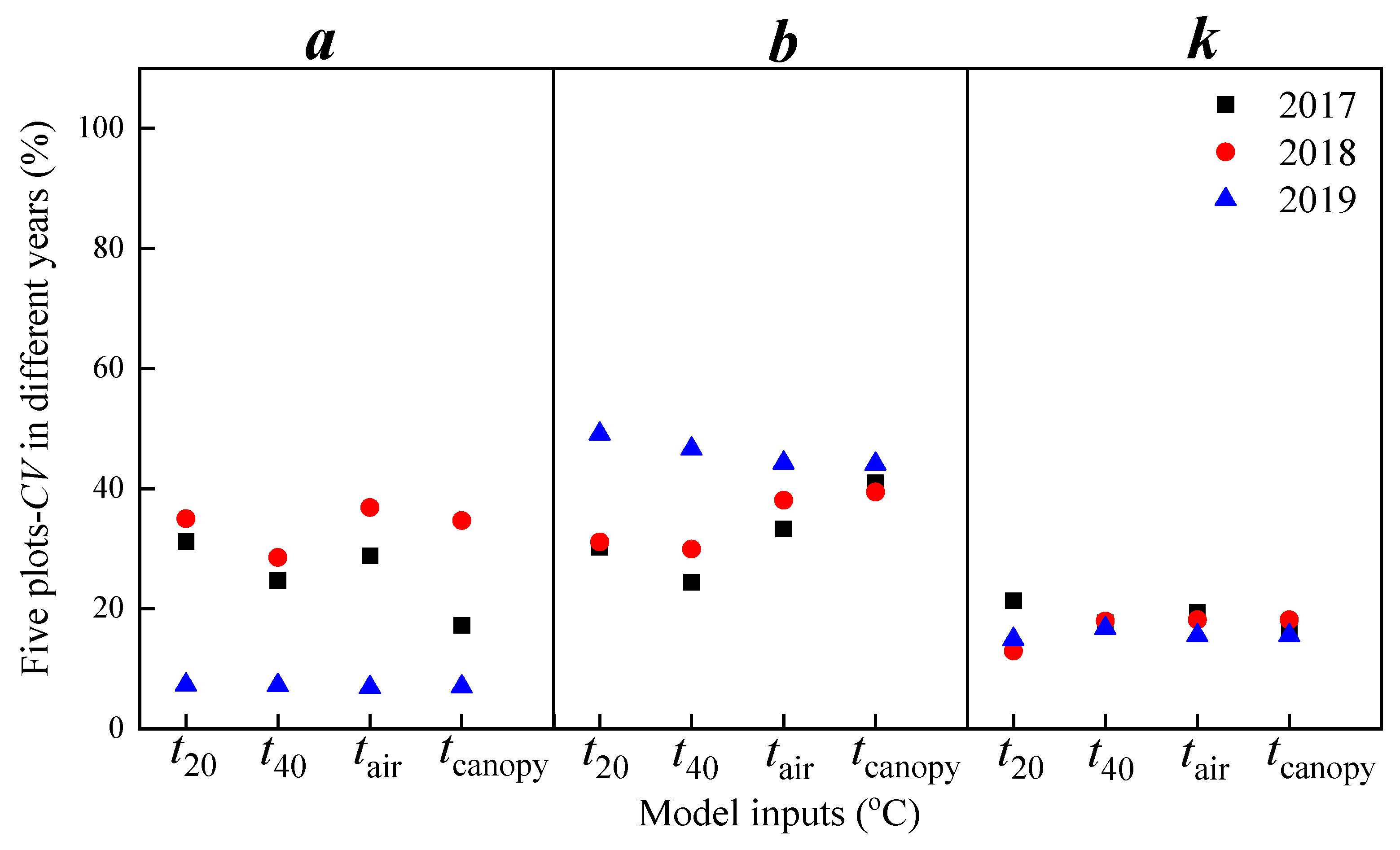
3.2.1. Calibration Results Based on the Logistic Model of DBA

Achieving high-quality estimates of DBA is necessary to predict crop yield. Using the logistic model, all of the DBA changes were simulated based on the field observations from 2017–2019. The simulations with four kinds of effective accumulated temperatures ran well, with R2 average values exceeding 0.95 for five plots (Figure 8a). Figure 8b shows the results of DBA simulating in 2017 of five plots by using tcanopy as model input. Each curve is extremely consistent with the measured values, revealing that it is feasible to realize crop growth monitoring by utilizing the Tc.
However, model parameters (a, b, and k) calibrated in different plots represent an obvious discrepancy, as shown in Figure 9, which provides the CV values for each parameter among five plots in different years. The CV values of a and b fluctuate significantly more than the k value. In addition, the tcanopy-based coefficients present as more stable due to lower CV values. Apparently, it is still hard to select universal model coefficients that best-simulate regional DBA owing to the existing variation in different plots and years.

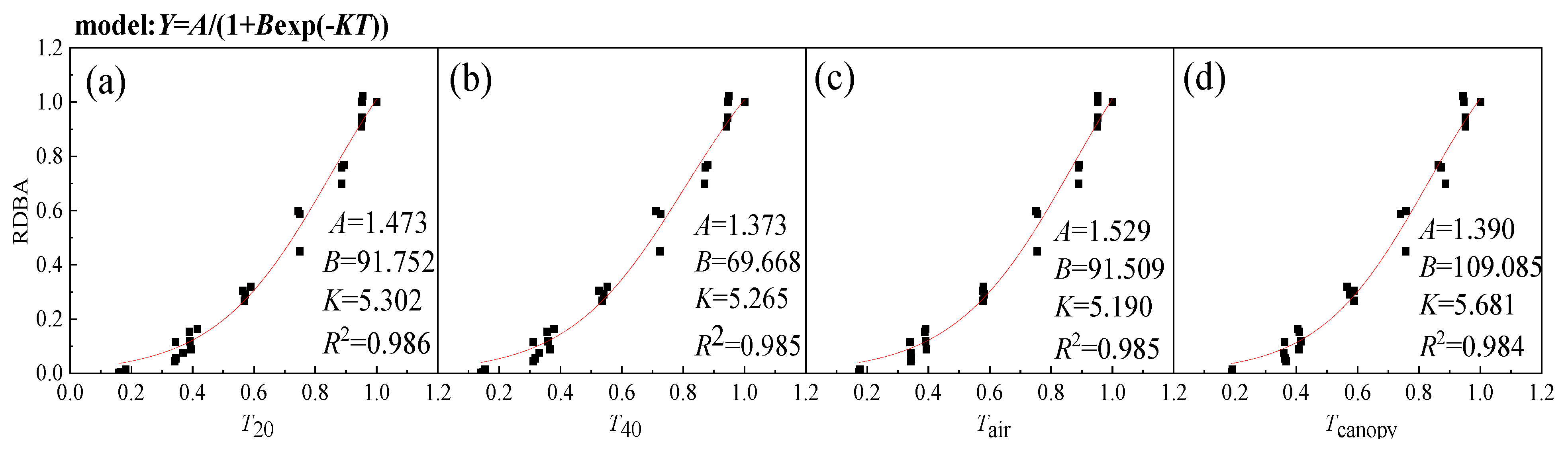
3.2.2. Calibration Results Based on the N-Logistic Model of RDBA

To address this issue, the N-logistic model was employed with different relative effective accumulated temperatures for the raw data from all the plots in 2017, 2018, and 2019 separately. The simulations for 2018 show the RDBA changes with T20, T40, Tair, and Tcanopy (Figure 10), in which high values of R2 (>0.98) suggest that it is feasible to simulate crop growth with good accuracy in regions when the data are normalized.
The calibrated results of the N-logistic model parameters with T20, T40, Tair, and Tcanopy in 2017–2019 presented the inter-annual differences of the model parameters, in which the CV values of A and K were relatively lower (Table 1). The results for Tcanopy performed better than other variables with lower CV values, suggesting that it is a good indicator to include.

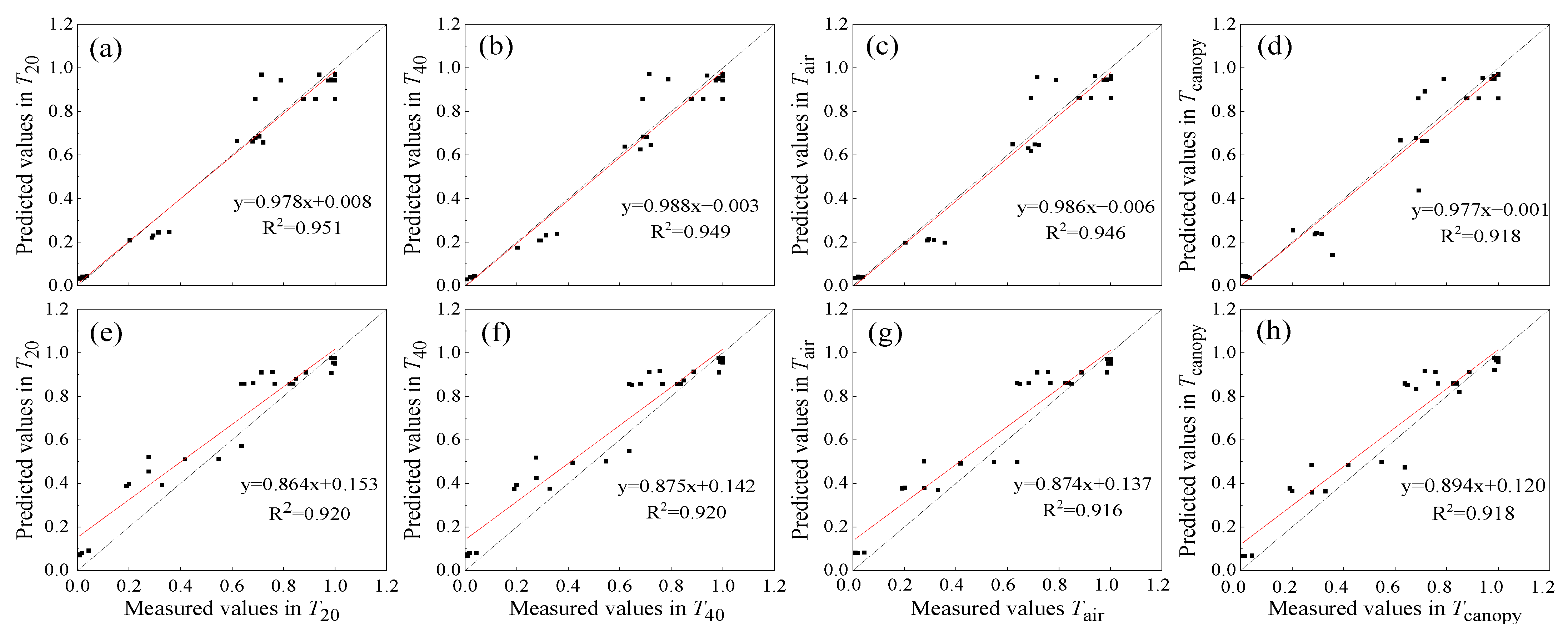
3.2.3. Validation Results Based on the N-Logistic Model of RDBA

To account for the inter-annual gap in the parameters of the N-logistic models, the calibrated models above were validated by the field observations of the other two years to identify the ideal set of regional parameters. A summary of the statistical characters of the N-logistic models with T20, T40, Tair, and Tcanopy is presented in Table 2.
For the calibrated models in 2017, the measured and predicted values were in better agreement in 2018 than in 2019 because of high values for d and R2 and low values of RMSE in 2018. The validation results for 2018 models were better in 2017 than in 2019. Likewise, the validation results in 2017 were better than in 2018 for the calibrated models in 2019. A comparison of all of the validation results showed that the statistical characters performed best in the calibrated models in 2019, with lower RMSE and RE and higher d and R2.
For the simulations based on Tcanopy, there were no large differences compared with T20, T40, and Tair (Table 2), suggesting that it is feasible to simulate RDBA during the growing season.

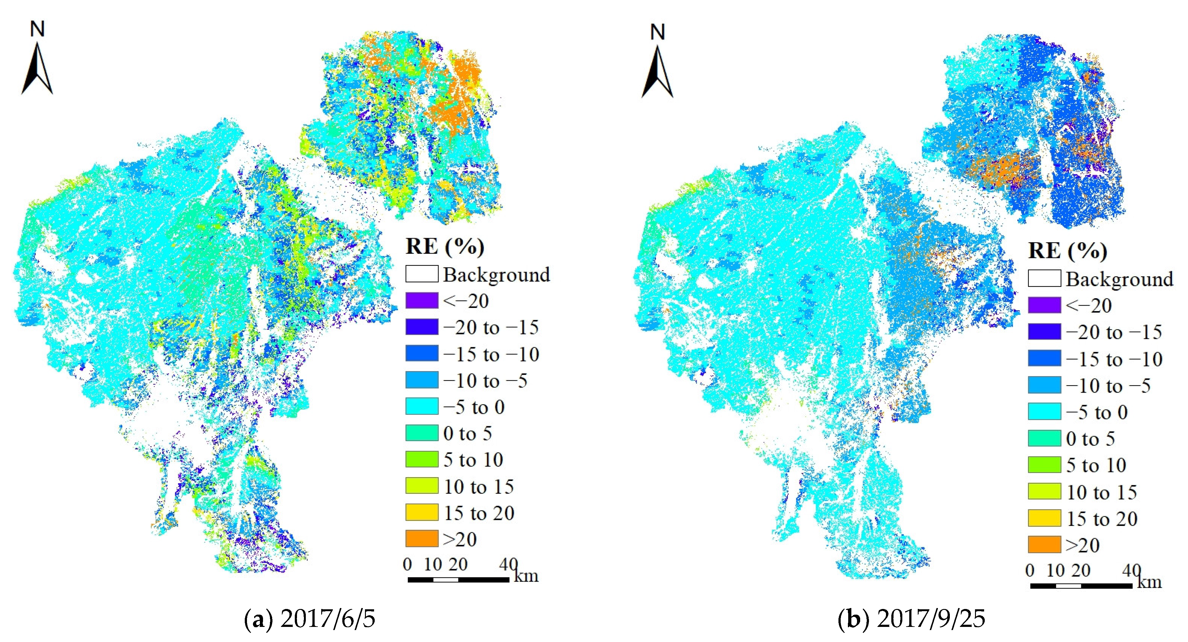
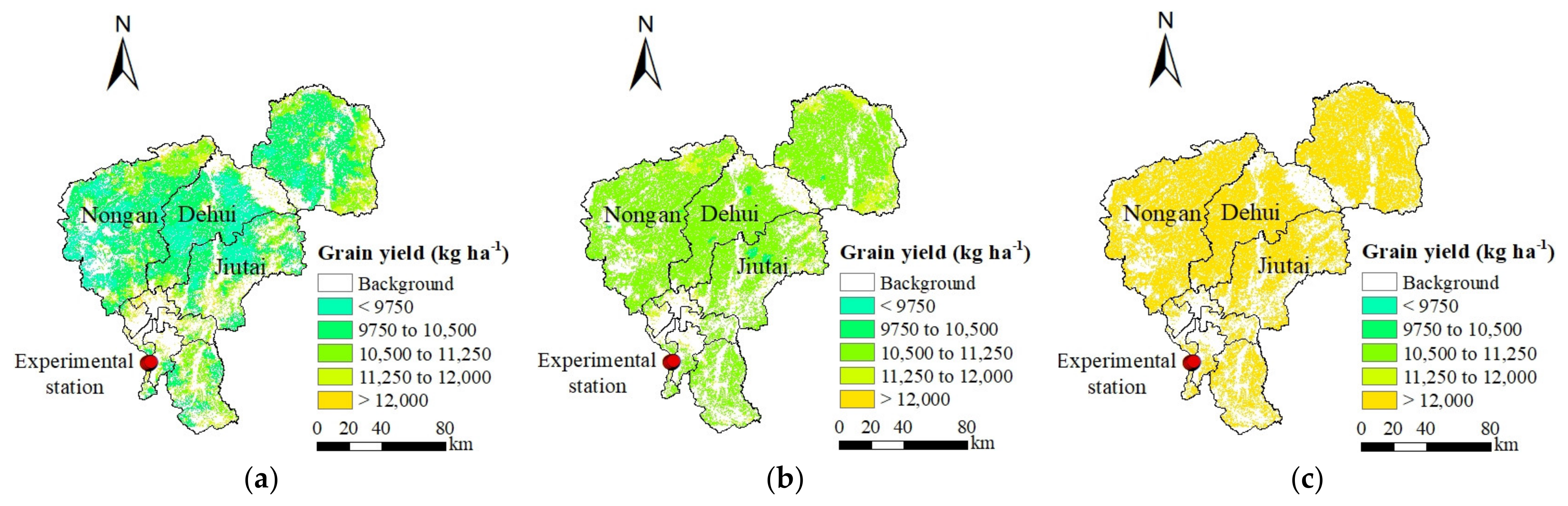
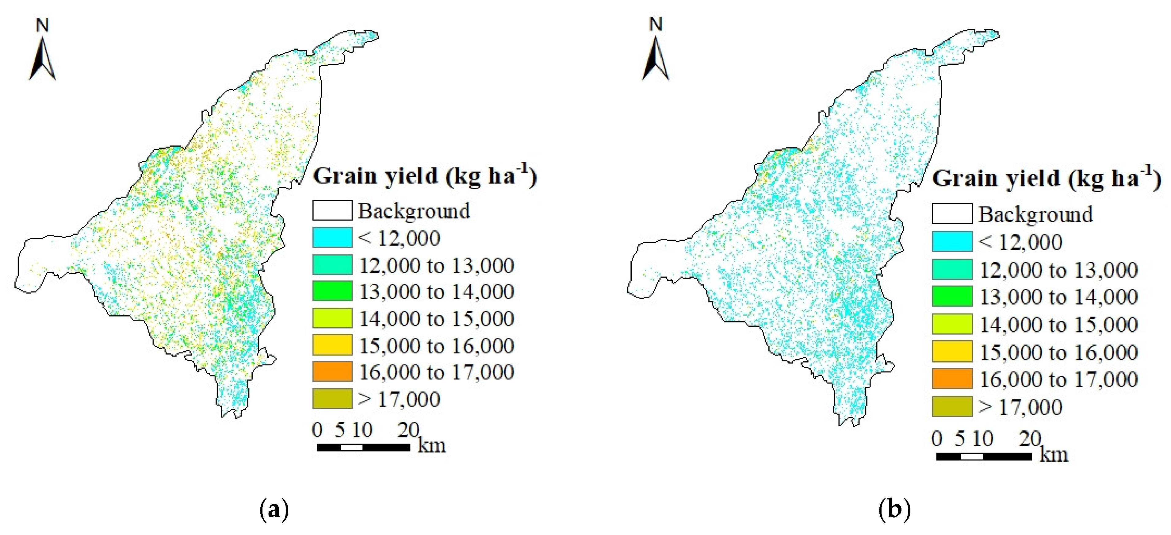
3.2.4. Grain Yield Forecasting in Area by MOD11A1-LST Values

Based on the results above, the validated N-logistic model for 2019 in Table 1 was used to simulate the pattern of RDBA in Changchun with Tcanopy, which was supposed to equal the TLST derived by the daily LST from MOD11A1. The y Dm (DBA at harvest) was ascertained by incorporating at least once-measured DBA ( y D ) in field through the growing season, and final grain yield could be forecasted then by the HI map. Here, the data in 2017 were used as an example to calculate and simulate to compare due to the limitation of research conditions and field observations.
Figure 11 demonstrates the spatial grain yield forecasted based on the field monitoring DBA of three different days in the growth period. Assimilating the DBA observation on 16 July into the model, the forecasted final grain yield was approximately 9750–10,500 kg ha−1 in most regions (Figure 11a). However, these values were 10,500–11,250 kg ha−1 and 12,000 kg ha−1 while assimilating the DBA observed on 10 August and 31 August (Figure 11b,c), respectively. As expected, assimilating closer to the harvest date enables the yield prediction to reach greater values, coinciding with the trend in crop growing.
These predicted results were compared with the measured maize grain yield from the reference of An [49], which provided an average value of grain yield of 11,364.3 kg ha−1 in three subareas of Dehui, Jiutai, and Nongan (Table 3). Simulated average values in the same regions in Figure 11 were 10,126.2 kg ha−1, 10,885.35 kg ha−1, and 13,492.8 kg ha−1, with corresponding RE values of −10.89%, −4.21%, and 18.73%, respectively. In addition, the simulated results were 10,778.57 kg ha−1, 10,976.90 kg ha−1, and 13,501.05 kg ha−1 based on the DBA values in three days at the experimental site, respectively. When such values were compared with the field yield observations (12,442.74 kg ha−1 on average here), then the values of RE were −13.38%, −11.78%, and 8.51% (Table 3), correspondingly. The yield prediction results confirm that the forecasting would be more precise along with the acquisition date of once-measured DBA closer to the harvest date.
It is significant for the accuracy of estimated results to choose the sampling time of DBA when the N-logistic model is used to estimate the grain yield in regions. In theory, the closer sampling time is to harvest time, the more accurate the yield estimate is. However, from the viewpoint of practical application, it is preferable to estimate grain yield early in the growth stage so as to promptly adjust the irrigation and agronomic management according to the estimated results.

3.3. Silage Yield Forecasting in Changchun

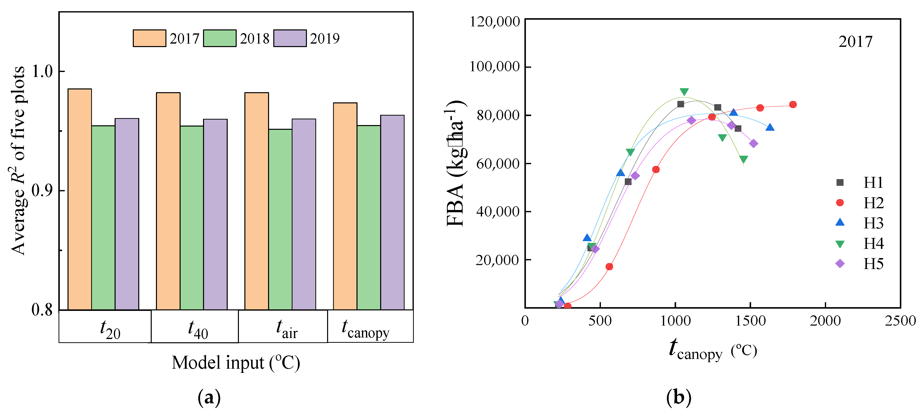
3.3.1. Calibration Results Based on the R-Logistic Model of FBA

Utilizing Equation (5), the FBA growth patterns were simulated and calibrated by the observed field values from 2017–2019. Similarly, the FBA simulations of each plot in three years based on the R-logistic model presented a high R2 (R2 > 0.95), indicating that the R-logistic model (previously applied to LAI growth) was capable of simulating the FBA patterns (Figure 12a). The FBA curves simulated in 2017 with the R-logistic model based on tcanopy are shown in Figure 12b. It is apparent that the curves of FBA included an exponential increase at the beginning of growth, followed by a bell-shaped pattern around the peak period, and then a decline toward physiological maturity (similar to LAI). Among them, the disparity in H2 performance could be attributed to sampling error. The maximum silage yield occurs at the peak of this curve, indicating that this may be an ideal harvest period if only the silage yield is considered.
However, the parameters of the calibrated model varied across years and plots. Figure 13 depicts the CV values for each model parameter among five plots in different years using the computation method consistent with Figure 9. Apparently, the CV values of all coefficients in R-logistic models appear to be higher than those in Figure 9. The reason for this result may be that the occurring time of maximum FBA (silage yield) is harder to pin down since farmers usually harvest silage maize in advance of full maturity.
In brief, the calibrated model by ontogenetic growth data struggles to explain regional maize growth because of the variation in model parameters between years and plots. Therefore, it is necessary to determine a set of universal model parameters for depicting maize growth in large areas.

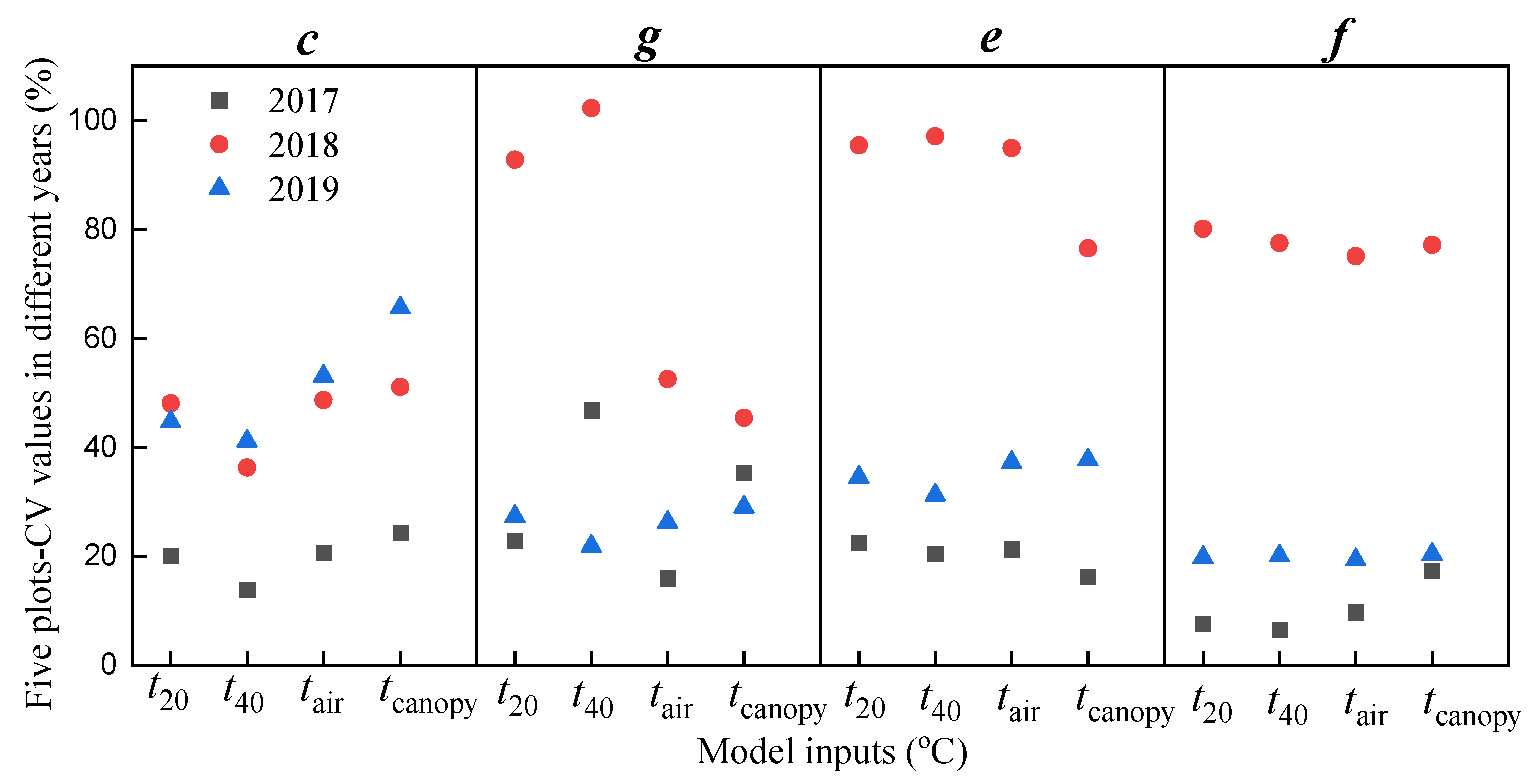
3.3.2. Calibration Results Based on the NR-Logistic Model of RFBA

The NR-logistic model was used to simulate the RFBA and to address the issues of regional application. All of the RFBA simulations were based on T20, T40, Tair, and Tcanopy for the raw data from 2017, 2018, and 2019 separately. During the results for 2017, the RFBA growth curve climbed to a peak and subsequently declined as the relative effective accumulated temperature increased (Figure 14). The values of R2 (>0.94) imply that it is acceptable to simulate RFBA in the research area with the model calibrated by the relative effective accumulated temperature. Meanwhile, no significant differences in R2 were found for models calibrated with T20, T40, Tair, and Tcanopy.
The RFBA and different relative effective accumulated temperatures in the five plots were used to calibrate the NR-logistic model each year. The calibration results for the model parameters with T20, T40, Tair, and Tcanopy are displayed in Table 4. The CV values in the model parameters G, E, and F were relatively lower than C, indicating different interannual variations in different parameters. The comparison of the parameters derived by different independent variables shows that the yearly gap of Tcanopy was lower, and the CV values of C, G, E, and F were 0.235, 0.047, −0.045, and 0.105, respectively.

3.3.3. Validation Results Based on the NR-Logistic Model of RFBA

Each NR-logistic model was validated by field observations of the other two years in order to test its performance in providing estimates of RFBA. The agreement between the measured and predicted values of the RFBA was evaluated via the statistical characters of RMSE, RE, R2, and d (Table 5). The calibrated model for 2017 was better validated in 2019 than in 2018, with lower values of RMSE and RE and higher values of d and R2. For the calibrated model in 2018, there were no differences between the validations in 2017 and 2019. However, the validation results for 2017 were better than in 2018 when using the calibrated model in 2019.
There were no extreme variations in the validated results of the calibrated model with T20, T40, Tair, and Tcanopy each year. The calibrated model in 2019 showed the optimal simulation precision for RFBA (compared to the other two years) even though it is somewhat poorer than the homologous model of RDBA in Table 2.
Using the NR-Logistic model calibrated in 2019 with T20, T40, Tair, and Tcanopy, a scatter plot of the predicted and measured values of RFBA in 2017 and 2018 was added to evaluate the model (Figure 15). The excellent agreement between them can be verified by the high R2 values (R2 > 0.92). Additionally, the R2 values were very close among the results for T20, T40, Tair, and Tcanopy. With respect to the results from 2017 (Figure 15a–d), as observed, the fitting data were evenly distributed on both sides of the 1:1 line, indicating a strong concordance between the measured and predicted RFBA. As for the results from 2018 (Figure 15e–h), the fitting data were somewhat over the 1:1 line, which showed that the RFBA was overestimated slightly. To summarize, the NR-logistic model calibrated in 2019 can predict the RFBA better in 2017 than in 2018.
The validated results with T20, T40, Tair, and Tcanopy and the model parameters (Table 4) can be used to assess the RFBA. The selection of the model independent variable may depend only on the way to monitor temperature in situ. The model application will be more convenient if the temperature can be collected easily. However, it is important to highlight that the Tc is a good factor for scale expansion.

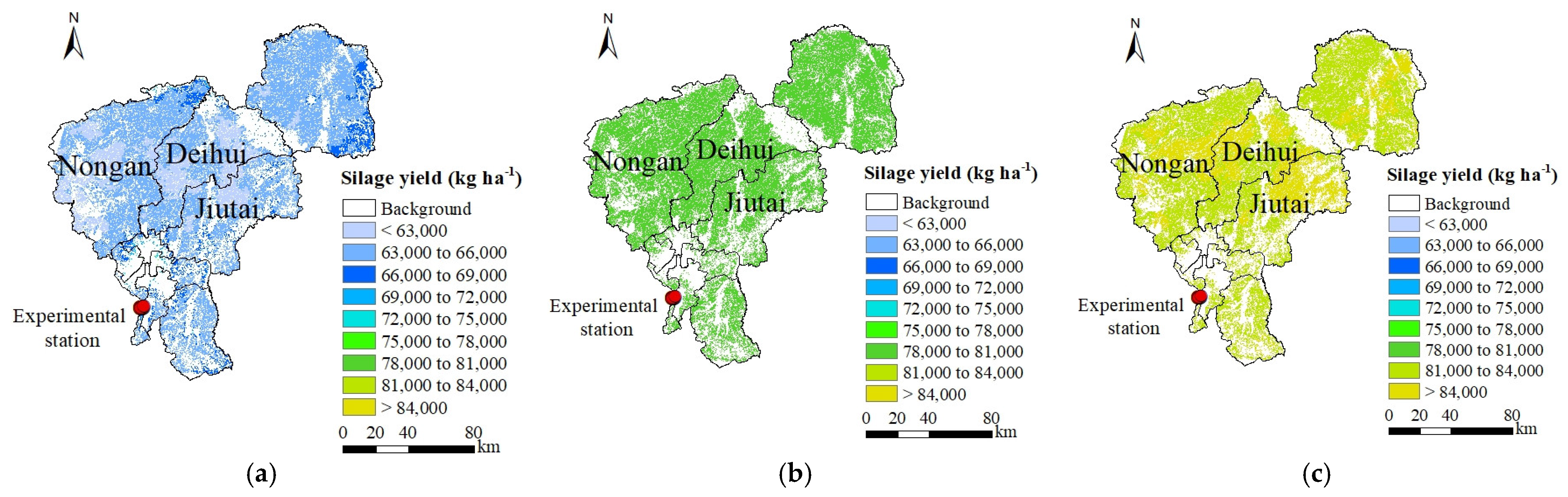
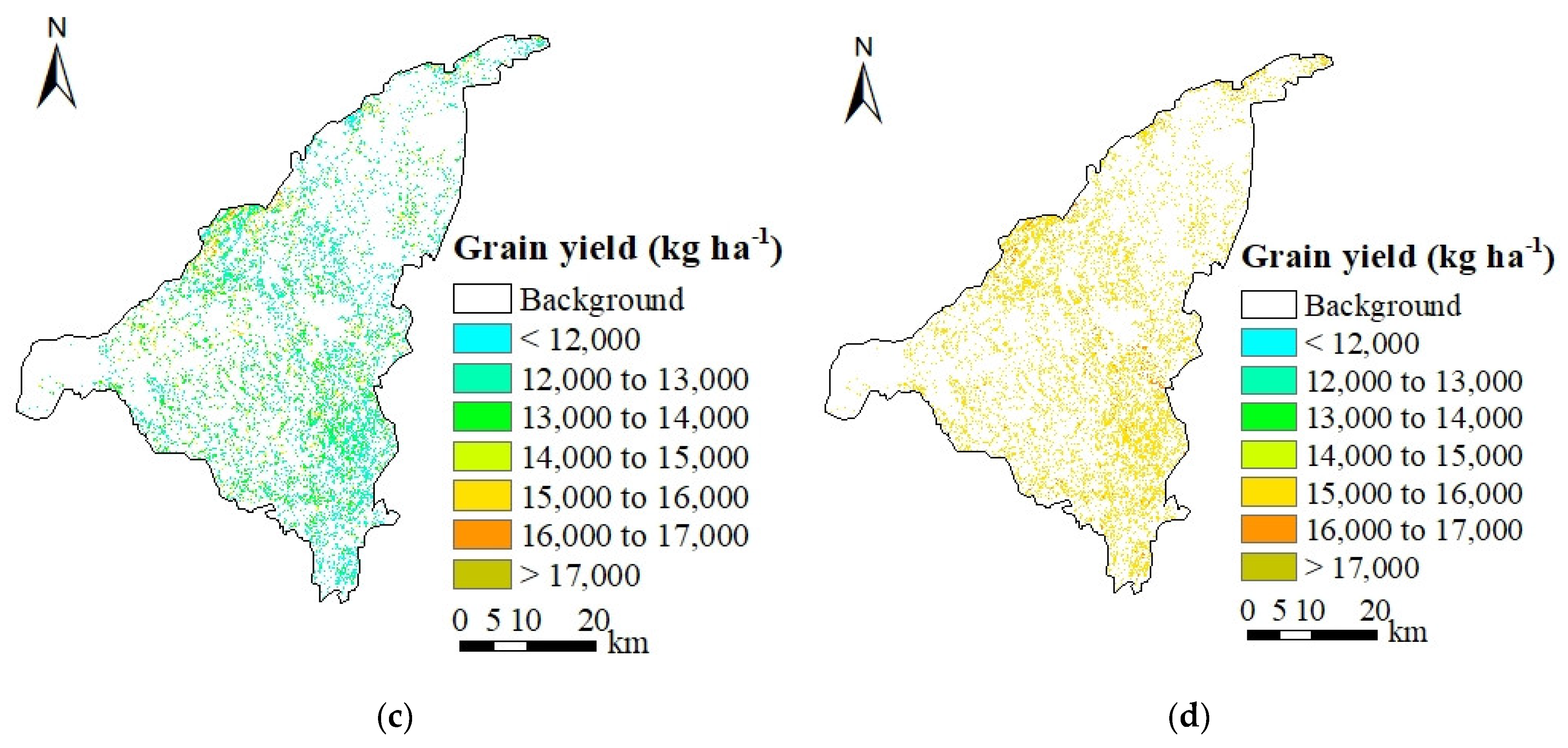
3.3.4. Silage Yield (Maximum FBA) Forecasting in Area by MOD11A1-LST Values

The shapes of the FBA and RFBA curves depicted above suggest that the silage yield should be near the peak of the curve to maximize profits. Therefore, the areal silage yield could be simulated by the validated Equation (6) in 2019 with TLST from MOD11A1 as a substitute for Tcanopy in combination with the field FBA observations on three different days at different growth stages (Figure 16). The differences in spatial distribution were captured. Similarly, the predicted FBA increased and got closer to the maximum output when the field observation date was near harvest.
According to the summarized data in Table 6, the model simulation showed only a slight difference on the observation day (31 August) in the experimental station. This is not surprising given that the measured silage yield was recorded on the same date. The results on 10 August still produced a satisfying accuracy, which indicates that it might be an appropriate harvest date for silage yield in view of various factors. There were no measurements of silage yield in the three subareas, so the comparison could not be analyzed and displayed between observations and predictions in the region.

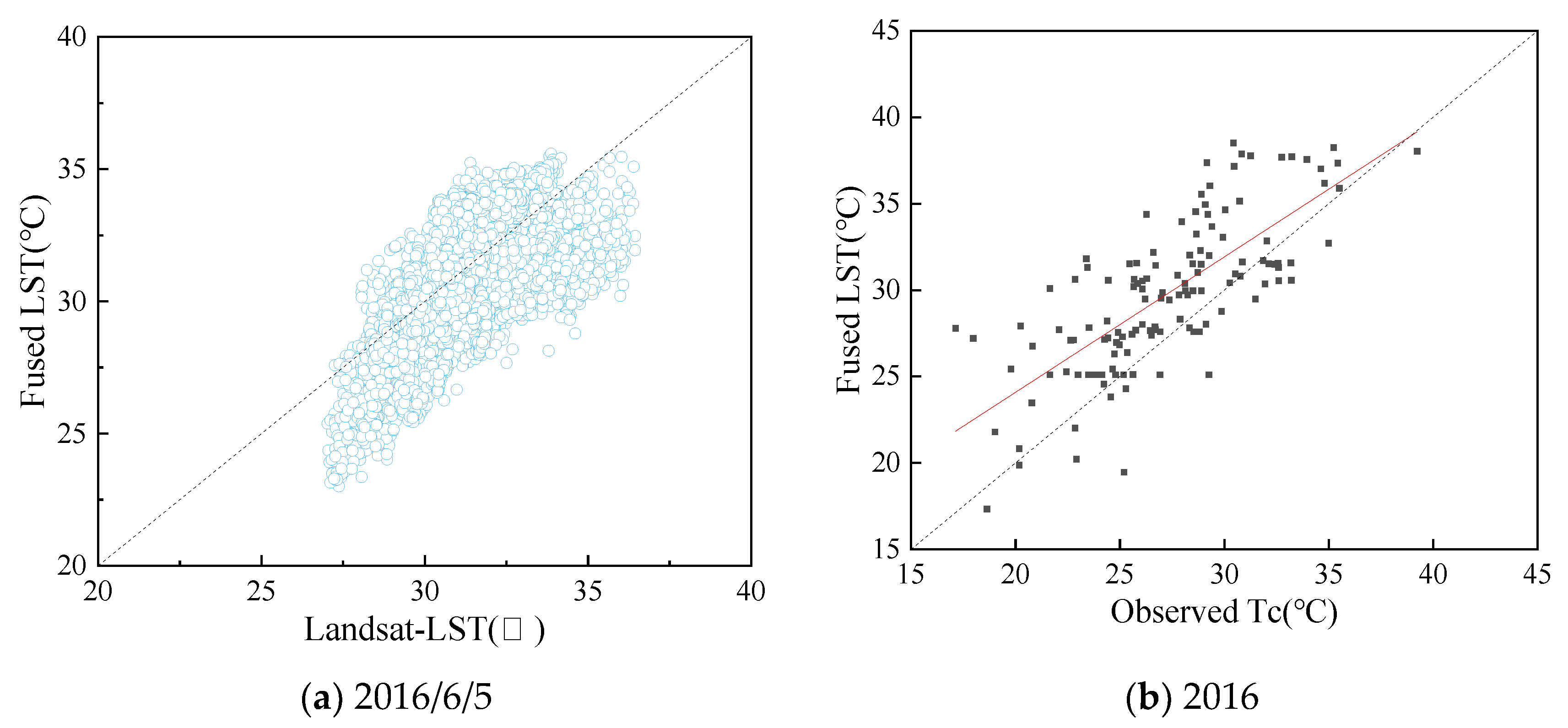
3.4. Verification in Jiefangzha Sub-Irrigation District

As mentioned in Section 2.3, an LST map (30 m) of Jiefangzha showed the results fused from Landsat 8 and MOD11A1 images by the ESTARFM algorithm. Scatters of the fused LSTs and Landsat-LSTs were evenly distributed on both sides of the 1:1 line, showing the fused LSTs were relatively reliable (Figure 17a). The fused LSTs were also compared with the Tc recorded at 11:30 a.m., in which the values of R2 (0.547), RMSE (3.96°C), and d (0.79) indicate good consistency between the observed values and the fused ones (Figure 17b). The grain yield forecasting map was constructed by employing the N-Logistic model described previously with the fused LSTs (Figure 18).
Figure 18 shows the spatial grain yield estimates retrieved using DBA measured on four acquisition dates that include (a) 4 July, (b) 21 July, (c) 4 August, and (d) 26 August in 2016 based on the model calibrated in 2019. The predicted yield showed a significant upward trend as the acquisition date of DBA approached harvest. Meanwhile, the comparisons between the predicted and measured yield in situ were conducted with statistical parameters as evaluation metrics of accuracy (Table 7). The predicted yields coincide with the measured ones with RE values, ranging from −16.14% to 9.84%, which confirms that assimilating once-measured data into the model can produce a great estimate of grain yield. Comparatively speaking, DBA assimilation closer to the harvest date allows for a more accurate prediction of yield except for the results based on the data on 21 July, which may be caused by the irrigation measures or the model parameters. Assimilating DBA measured on 4 July also provides a reliable result, albeit with a slightly lower R2. Such a result proves the feasibility of the approach for early yield forecasting in other large areas though the optimal date of sampling still needs to be explored and determined further.

4. Discussion

According to results reported above, our data on maize biomass show that the Tc should be included as a valuable proxy of other independent variables in models because the Tc can be recognized as LST in large regions covered by maize that can be derived from remote sensing data [50,51].
This study demonstrated the benefits of integrating remote sensing LST into crop growth models in combination with once-observed values (DBA or FBA) to enhance yield prediction. The introduction of remote sensing LST to the logistic models offers effective information about regional crop status, overcoming the limitation of model in regional application. Moreover, the ground crop truth was profitably considered by using once-measured observations as the drive of the yield forecasting model. Another point worth emphasizing is that the subsequent consequences, after undertaking necessary agronomic measures based on the yield forecasting results, can be assessed with just one observation as input again because the effect on the crop can be reflected by LST and measured biomass. All in all, LST as a key factor for characterizing field drought [52] provides an intuitive basis to determine the water shortage of crops in large regions. This offers a solid theoretical basis for the synergistic prediction of future crop drought and yield evaluation in combination using remote sensing technology.
In addition, to obtain a more robust estimate of maize yield, data fusion technology may be recommended to improve the spatio-temporal resolution of LST [40]. Unfortunately, this method is unavailable due to the scarce Landsat images caused by the cloud cover on most days in maize growing season in Changchun. Our attempt in the Jiefangzha sub-irrigation district indicated that the data fusion technology improved the performance of spatial variation of grain yield forecasting under available conditions of suitable Landsat images. It follows that high-resolution satellite imagery such as Sentinel-2 might be a further exploration tool for improving yield forecasting precision.
The values of tm in models of RDBA and RFBA are key input data, which can be obtained for different hydrological years by analysis of the local yearly rainfall. When the hydrological year of the current growing season is estimated, the N-logistic model and the NR-logistic model can be utilized with the corresponding value of tm. To obtain the values of y Dm and y Fm , the data of DBA and FBA should be collected in field at least once during the maize growing period. Furthermore, the growth patterns of DBA and FBA can be simulated when the models are set up and calibrated. HI, an empirical value describing the relationship between DBA and grain yield, offers an opportunity to evaluate grain yield. By combining the growth curves for DBA and FBA with the future market demands, maize can be flexibly harvested as silage or grain during the growing season.
Apparently, the early yield forecasting accuracy varies depending on the growth stages, which may be caused by many factors. Firstly, the retrieval of tm is pivotal, as mentioned above. Secondly, the quality of remote sensing images obtained over time varies slightly, which can introduce some uncertainty into the yield forecasting results. Thirdly, the date of acquiring DBA or FBA is particularly critical for yield forecasting accuracy. As shown in Table 3 and Table 7, the optimal predicting date is clearly different in different areas. In Changchun, the optimal date at which the DBA provides more accurate yield forecasting is approximately 38 days (10 August) ahead of harvest. As for the Jiefangzha sub-irrigation district, the results on 26 August produced a better prediction of yield, relatively speaking. Furthermore, the latter is better than the former in statistical parameters. This phenomenon may be caused by a variety of factors. For instance, a rare downpour amounting to more than 160 mm of rain occurred in Changchun on 21 July 2017, which may destroy plants and influence yield forecasting results. In addition, the area of Changchun is larger than the Jiefangzha sub-irrigation district, which may have an impact on the results. Taking the three results into account (Table 3, Table 6 and Table 7), it is suggested to forecast yield by using the field data (DBA or FBA) measured at the middle growth period (early August). Furthermore, it is necessary to determine the optimal date by taking into consideration multiple factors.
Another noteworthy point about the results presented here is that the field soil water content was sufficient or at least was not in water deficit in the research area. The FBA, RFBA, and silage yield may be impacted by the crop and soil water conditions. Future efforts to prove model generality should include examination of changes in the model parameters for different levels of plant and field soil moisture.

5. Conclusions

An approach for yield forecasting from plot level to large scale was developed by incorporating remote sensing LST of a measured biological indicator (DBA and FBA) into corresponding logistic models. The main conclusions are as follows:
(1)
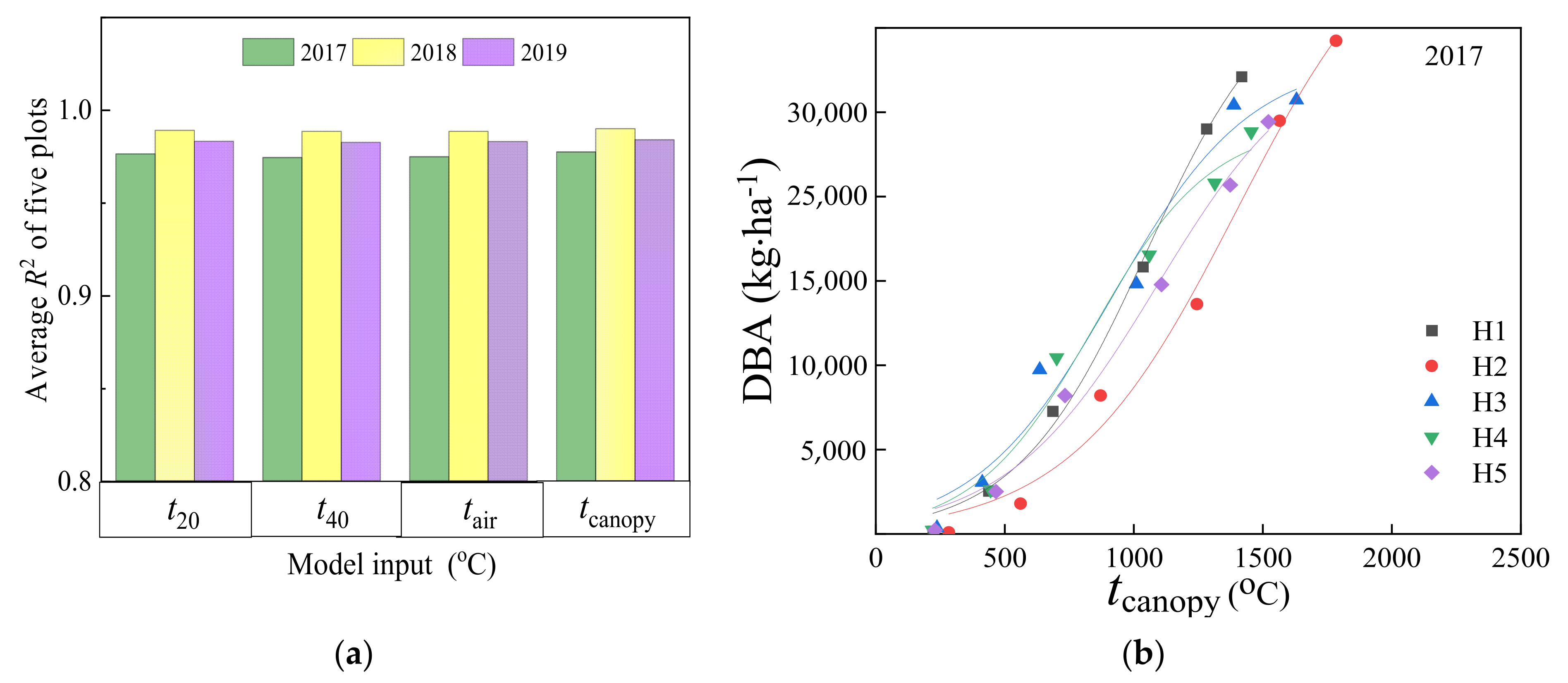
The model of 2019 based on Tcanopy performed better result than others. Crop canopy temperature can be used as input parameter in logistic models to simulate DBA and FBA. It is thus a potentially valuable index to facilitate model development in regions.
(2)
The normalization method can eliminate the difference in temporal scale between measured daily average values of Tc and instantaneous remote sensing LSTs. Therefore, the normalized LST retrieved from MOD11A1 can be used directly as an independent variable in models to simulate crop biomass for yield forecasting in areas.
(3)
The yield forecasting accuracy is reliable in regions with this approach. Satisfactory grain and silage yield forecasting in Changchun were provided by assimilating DBA or FBA measured on 10 August ahead of harvest with RE values of −4.21% and −6.1%, respectively.
(4)
The application in the Jiefangzha sub-irrigation district demonstrated that it is possible to apply this approach to predict yield in other regions. These simulation results hold broad potential to provide a real-time reference in maize growing stages for farmers and the grain futures market to make decisions.

Supplementary Materials

The following supporting information can be downloaded at: https://www.mdpi.com/article/10.3390/rs15041025/s1, Figure S1: Rules of decision tree classification for Landsat8 images based on the values of NDVI and LSWI in ROI in 2017 (No.268 (2017/9/25) and No.156 (2017/6/5)); Figure S2: Map of HI obtained by the kriging interpolation method in Changchun area; Figure S3: Regressions between the LST from MOD11A1 product and the observed Tc in field in 2017. (a) H4; (b) H5; Figure S4: Regressions between the TLST calculated by the remote sensing instantaneous LST values at 11:30 a.m. (interpolation results) and daily average values observed (Tcanopy) from the CTMS system in 2017. (a) H4; (b) H5; Table S1: Data list of remote sensing images in 2017; Table S2: Values of harvest index (HI) of maize collected or measured in Changchun and its surrounding areas; Equations (S1)–(S5): Supplementary calculation formula of Section 2.6.

Author Contributions

Conceptualization, J.C.; data curation, H.C.; formal analysis, J.C.; funding acquisition, B.Z.; investigation, H.C.; methodology, H.C.; project administration, Z.W.; resources, J.C.; supervision, D.X.; validation, H.C.; writing—original draft, H.C.; writing—review and editing, J.C. All authors have read and agreed to the published version of the manuscript.

Funding

This research was funded by the National Key Research Program (grant number NK2022180403), the Project of National Natural Science Foundation of China (grant numbers 52130906, 51979286), and the Institute-City Cooperation Program (grant number HBAT02242202010-CG).

Data Availability Statement

The data that support the findings of this work are available from the corresponding author upon reasonable request.

Acknowledgments

The authors would like to thank the anonymous reviewers for their long-term guidance and constructive comments. The authors are grateful to the Ministry of Natural Resources of China for providing the land-cover map in Changchun and the Statistic Bureau of Jilin Province for providing the statistical data of crop areas. The authors also acknowledge the United States Geological Survey (USGS) for offering the images of Landsat 8 and MOD11A1 products.

Conflicts of Interest

The authors declare no conflict of interest.

Abbreviations

LSTLand surface temperature, °C
TcCanopy temperature, °C
DBADry biomass accumulation, kg ha−1
FBAFresh biomass accumulation, kg ha−1
LAILeaf area index
RDBARelative dry biomass accumulation
HIHarvest index
RFBARelative fresh biomass accumulation
FcField capacity
WpWilting point
CTMSCanopy temperature and meteorology monitoring systems
NDVINormalized difference vegetation index
LSWILand surface water index
ROIRegion of interest
ƿ N I R Reflectivity of near-infrared band
ƿ R E D Reflectivity of red band
ƿ S W I R Reflectivity of shortwave infrared band
y D Dependent growth parameter
tEffective accumulated temperature after emergence, °C
t i Mean daily temperature in the air, canopy, or soil at 20 cm or 40 cm in the root zone, °C
aThe theoretical upper limit of growth of dry biomass accumulation
b,kParameters of the logistic model
tairEffective accumulative air temperature, °C
tcanopyEffective accumulative canopy temperature, °C
t20Effective accumulative soil temperature at 20 cm in root zone, °C
t40Effective accumulative soil temperature at 40 cm in root zone, °C
TRelative effective accumulated temperature
YDRelative dry biomass accumulation
y Dm Dry biomass accumulation at harvest, kg ha−1
t m Effective accumulative temperature at harvest, °C
AThe upper limit of relative dry biomass accumulation
B, KParameters of the normalized logistic model
T20Relative effective accumulative soil temperature at 20 cm in root zone
T40Relative effective accumulative soil temperature at 40 cm in root zone
TcanopyRelative effective accumulative canopy temperature
TairRelative effective accumulative air temperature
y F Above-ground fresh biomass accumulation, kg ha−1
c, g, e, fParameters of the revised logistic model
Y F Relative fresh biomass accumulation
y Fm Maximum relative fresh biomass accumulation
C, G, E, FParameters of the normalized revised logistic model
YGrain yield, kg ha−1
TLSTThe relative effective accumulative canopy temperature calculated by the remote sensing instantaneous values of MOD11A1
dIndex of agreement
RMSERoot mean square error
RERelative error
R2Coefficient of determination
CVCoefficient of variation

References

  1. Chen, Y.; Tao, F.L. Potential of remote sensing data-crop model assimilation and seasonal weather forecasts for early-season crop yield forecasting over a large area. Field Crop. Res. 2022, 276, 108398. [Google Scholar] [CrossRef]
  2. Ziliani, M.G.; Altaf, M.U.; Aragon, B.; Houborg, R.; Franz, T.E.; Lu, Y.; Sheffield, J.; Hoteit, I.; McCabe, M.F. Early season prediction of within-field crop yield variability by assimilating CubeSat data into a crop model. Agric. For. Meteorol. 2022, 313, 108736. [Google Scholar] [CrossRef]
  3. Basso, B.; Liu, L. Chapter Four—Seasonal crop yield forecast: Methods, applications, and accuracies. Adv. Agron. 2019, 154, 201–255. [Google Scholar] [CrossRef]
  4. Liu, Y.Q.; Song, W. Modelling crop yield, water consumption, and water use efficiency for sustainable agroecosystem management. J. Clean. Prod. 2020, 253, 119940. [Google Scholar] [CrossRef]
  5. Paudel, D.; Boogaard, H.; Wit, A.D.; Janssen, S.; Osinga, S.; Pylianidis, C.; Athanasiadis, I.N. Machine learning for large-scale crop yield forecasting. Agric. Syst. 2021, 187, 103016. [Google Scholar] [CrossRef]
  6. Hoogenboom, G. Contribution of agrometeorology to the simulation of crop production and its applications. Agric. For. Meteorol. 2000, 103, 137–157. [Google Scholar] [CrossRef]
  7. Liu, S.; Yang, J.Y.; Drury, C.F.; Liu, H.L.; Reynolds, W.D. Simulating maize (Zea mays L.) growth and yield, soil nitrogen concentration, and soil water content for a long-term cropping experiment in Ontario, Canada. Can. J. Soil Sci. 2014, 94, 435–452. [Google Scholar] [CrossRef]
  8. Mubeen, M.; Ahmad, A.; Wajid, A.; Khalip, T.; Hammad, H.M.; Sultana, S.R.; Ahmad, S.; Fahad, S.; Nasim, W. Application of CSM-CERES-Maize model in optimizing irrigated conditions. Outlook Agric. 2016, 45, 173–184. [Google Scholar] [CrossRef]
  9. Wu, W.; Chen, J.L.; Liu, H.B.; Garcia, A.G.; Hoogenboom, G. Parameterizing soil and weather inputs for crop simulation models using the VEMAP database. Agric. Ecosyst. Environ. 2010, 135, 111–118. [Google Scholar] [CrossRef]
  10. Birch, C.P.D. A new generalized Logistic sigmoid growth equation compared with the Richards growth equation. Ann. Bot. 1999, 83, 713–723. [Google Scholar] [CrossRef] [Green Version]
  11. West, G.B.; Brown, J.H.; Enquist, B.J. A general model for ontogenetic growth. Nature 2001, 413, 628–631. [Google Scholar] [CrossRef]
  12. Bontemps, J.; Duplat, P. A non-asymptotic sigmoid growth curve for top height growth in forest stands. Forestry 2012, 85, 353–368. [Google Scholar] [CrossRef]
  13. Lewis, J.M.; Lakshmivarahan, S.; Dhall, S. Dynamic Data Assimilation: A Least Squares Approach; Cambridge University Press: Cambridge, UK, 2006; Available online: http://www.gbv.de/dms/goettingen/508439248.pdf (accessed on 16 March 2022).
  14. Schwalbert, R.A.; Amado, T.J.C.; Nieto, L.; Varela, S.; Corassa, G.M.; Horbe, T.A.N.; Rice, C.W.; Peralta, N.R.; Ciampitti, I.A. Forecasting maize yield at field scale based on high-resolution satellite imagery. Biosyst. Eng. 2018, 171, 179–192. [Google Scholar] [CrossRef]
  15. Sharifi, A. Yield prediction with machine learning algorithms and satellite images. J. Sci. Food Agric. 2021, 101, 891–896. [Google Scholar] [CrossRef]
  16. Veloso, A.; Mermoz, S.; Bouvet, A.; Toan, T.L.; Planells, M.; Dejoux, J.-F.; Ceschia, E. Understanding the temporal behavior of crops using Sentinel-1 and Sentinel-2-like data for agricultural applications. Remote Sens. Environ. 2017, 199, 415–426. [Google Scholar] [CrossRef]
  17. Gaso, D.V.; Wit, A.D.; Berger, A.G.; Kooistra, L. Predicting within-field soybean yield variability by coupling Sentinel-2 leaf area index with a crop growth model. Agric. For. Meteorol. 2021, 308–309, 108553. [Google Scholar] [CrossRef]
  18. Jin, N.; Tao, B.; Ren, W.; He, L.; Zhang, D.Y.; Wang, D.H.; Yu, Q. Assimilating remote sensing data into a crop model improves winter wheat yield estimation based on regional irrigation data. Agric. Water Manag. 2022, 266, 107583. [Google Scholar] [CrossRef]
  19. Liu, Z.C.; Wang, C.; Bi, R.T.; Zhu, H.F.; He, P.; Jing, Y.D.; Yang, W.D. Winter wheat yield estimation based on assimilated Sentinel-2 images with the CERES-Wheat model. J. Integr. Agric. 2021, 20, 1958–1968. [Google Scholar] [CrossRef]
  20. Zhuo, W.; Huang, J.X.; Xiao, X.M.; Huang, H.; Bajgain, R.; Wu, X.C.; Gao, X.R.; Wang, J.; Li, X.C.; Wagle, P. Assimilating remote sensing-based VPM GPP into the WOFOST model for improving regional winter wheat yield estimation. Eur. J. Agron. 2022, 139, 126556. [Google Scholar] [CrossRef]
  21. Junior, I.M.F.; Vianna, M.D.S.; Marin, F.R. Assimilating leaf area index data into a sugarcane process-based crop model for improving yield estimation. Eur. J. Agron. 2022, 136, 126501. [Google Scholar] [CrossRef]
  22. Klopfenstein, T.J.; Erickson, G.E.; Berger, L.L. Maize is a critically important source of food, feed, energy and forage in the USA. Field Crop. Res. 2013, 153, 5–11. [Google Scholar] [CrossRef]
  23. Yan, D.C.; Zhu, Y.; Wang, S.H.; Cao, W.X. A quantitative knowledge-based model for designing suitable growth dynamics in rice. Plant Prod. Sci. 2006, 9, 93–105. [Google Scholar] [CrossRef]
  24. Sheehy, J.E.; Mitchel, P.L.; Allen, L.H.; Ferrer, A.B. Mathematical consequences of using various empirical expressions of crop yield as a function of temperature. Field Crop. Res. 2006, 98, 216–221. [Google Scholar] [CrossRef]
  25. Singer, J.W.; Meek, D.W.; Sauer, T.J.; Prueger, J.H.; Hatfield, J.L. Variability of light interception and radiation use efficiency in maize and soybean. Field Crop. Res. 2011, 121, 147–152. [Google Scholar] [CrossRef]
  26. Shi, P.J.; Men, X.Y.; Sandhu, H.S.; Chakraborty, A.; Li, B.L.; Ou-Yang, F.; Sun, Y.C.; Ge, F. The “general” ontogenetic growth model is inapplicable to crop growth. Ecol. Model. 2013, 266, 1–9. [Google Scholar] [CrossRef]
  27. Bakoglu, A.; Celik, S.; Kokten, K.; Kilic, O. Examination of plant length, dry stem and dry leaf weight of bitter vetch [Vicia ervilia (L) Willd.] with some non-linear growth models. Legume Res. 2016, 39, 533–542. [Google Scholar] [CrossRef]
  28. Wang, X.L. How to utilize Logistic model in dynamic simulation of crop dry biomass accumulation. Chin. J. Agrometeorol. 1986, 7, 14–19. (In Chinese) [Google Scholar]
  29. Liu, Y.H.; Su, L.J.; Wang, Q.J.; Zhang, J.H.; Shan, Y.Y.; Deng, M.J. Chapter Six—Comprehensive and quantitative analysis of growth characteristics of winter wheat in China based on growing degree days. Adv. Agron. 2020, 159, 237–273. [Google Scholar] [CrossRef]
  30. Elings, A. Estimation of leaf area in tropical maize. Agron. J. 2000, 92, 436–444. [Google Scholar] [CrossRef]
  31. Yu, Q.; Liu, J.D.; Zhang, Y.Q.; Li, J. Simulation of rice biomass accumulation by an extended Logistic model including influence of meteorological factors. Int. J. Biometeorol. 2002, 46, 185–191. [Google Scholar] [CrossRef]
  32. Sepaskhah, A.R.; Fahandezh-Saadi, S.; Zand-Parsa, S. Logistic model application for prediction of maize yield under water and nitrogen management. Agric. Water Manag. 2011, 99, 51–57. [Google Scholar] [CrossRef]
  33. Shabani, A.; Sepaskhah, A.R.; Kamgar-Haghighi, A.A. Estimation of yield and dry matter of rapeseed using Logistic model under water, salinity and deficit irrigation. Arch. Agron. Soil Sci. 2014, 60, 951–969. [Google Scholar] [CrossRef]
  34. Mahbod, M.; Sepaskhah, A.R.; Zand-Parsa, S. Estimation of yield and dry matter of winter wheat using Logistic model under different irrigation water regimes and nitrogen application rates. Arch. Agron. Soil Sci. 2014, 60, 1661–1676. [Google Scholar] [CrossRef]
  35. Mayer, F.; Gerin, P.A.; Noo, A.; Foucart, G.; Flammang, J.; Lemaigre, S.; Sinnaeve, G.; Dardenne, P.; Delfosse, P. Assessment of factors influencing the biomethane yield of maize silages. Bioresour. Technol. 2014, 153, 260–268. [Google Scholar] [CrossRef] [PubMed]
  36. Pede, T.; Mountrakis, G.; Shaw, S.B. Improving corn yield prediction across the US Corn Belt by replacing air temperature with daily MODIS land surface temperature. Agric. For. Meteorol. 2019, 276–277, 107615. [Google Scholar] [CrossRef]
  37. Cai, J.B.; Xu, D.; Si, N.; Wei, Z. Real-time monitoring system of crop canopy temperature and soil moisture for irrigation decision-making. T. Chin. Soc. Agric. Mach. 2015, 46, 133–139, (In Chinese with English abstract). [Google Scholar] [CrossRef]
  38. Qi, L.L. Research on Safety of Water Supply in Chang-Ji Economic Circle. Master’s Thesis, Jilin University, Changchun, China, 2019. (In Chinese with English abstract). [Google Scholar]
  39. Bai, L.L.; Cai, J.B.; Liu, Y.; Chen, H.; Zhang, B.Z.; Huang, L.X. Responses of field evapotranspiration to the changes of cropping pattern and groundwater depth in large irrigation district of Yellow River basin. Agric. Water Manag. 2017, 188, 1–11. [Google Scholar] [CrossRef]
  40. Huang, L.X.; Cai, J.B.; Zhang, B.Z.; Chen, H.; Bai, L.L.; Wei, Z.; Peng, Z.G. Estimation of evapotranspiration using the crop canopy temperature at field to regional scales in large irrigation district. Agric. For. Meteorol. 2019, 269–270, 305–322. [Google Scholar] [CrossRef]
  41. Xiao, X.M.; Zhang, Q.Y.; Braswell, B.; Urbanski, S.; Boles, S.; Wofsy, S.; Moore, B.; Ojima, D. Modeling gross primary production of a deciduous broadleaf forest using satellite images and climate data. Remote Sens. Environ. 2004, 91, 256–270. [Google Scholar] [CrossRef]
  42. Chandrasekar, K.; Sesha Sai, M.V.R.; Roy, P.S.; Dwevedi, R.S. Land Surface Water Index (LSWI) response to rainfall and NDVI using the MODIS Vegetation Index product. Int. J. Remote Sens. 2010, 31, 3987–4005. [Google Scholar] [CrossRef]
  43. Zhu, X.L.; Chen, J.; Gao, F.; Chen, X.H.; Masek, J.G. An enhanced spatial and temporal adaptive reflectance fusion model for complex heterogeneous regions. Remote Sens. Environ. 2010, 114, 2610–2623. [Google Scholar] [CrossRef]
  44. Wu, R.L.; Ma, C.-X.; Chang, M.; Littell, R.C.; Wu, S.S.; Yin, T.M.; Huang, M.R.; Wang, M.X.; Casella, G. A Logistic mixture model for characterizing genetic determinants causing differentiation in growth trajectories. Genet. Res. 2002, 79, 235–245. [Google Scholar] [CrossRef] [PubMed]
  45. Zhao, J.F.; Guo, J.P.; Mu, J. Exploring the relationships between climatic variables and climate-induced yield of spring maize in Northeast China. Agric. Ecosyst. Environ. 2015, 207, 79–90. [Google Scholar] [CrossRef]
  46. Ding, D.Y.; Feng, H.; Zhao, Y.; Hill, R.L.; Yan, H.M.; Chen, H.X.; Hou, H.J.; Chu, X.S.; Liu, J.C.; Wang, N.J.; et al. Effects of continuous plastic mulching on crop growth in a winter wheat-summer maize rotation system on the loess plateau of China. Agric. For. Meteorol. 2019, 271, 385–397. [Google Scholar] [CrossRef]
  47. Meade, K.A.; Cooper, M.; Beavis, W.D. Modeling biomass accumulation in maize kernels. Field Crop. Res. 2013, 151, 92–100. [Google Scholar] [CrossRef]
  48. Liu, Y.; Li, Y.F.; Li, J.S.; Yan, H.J. Effects of mulched drip irrigation on water and heat conditions in field and maize yield in sub-humid region of Northeast China. T. Chin. Soc. Agric. Mach. 2015, 46, 93–104, 135, (In Chinese with English abstract). [Google Scholar] [CrossRef]
  49. An, Q. Research on Methods of Maize Yield Estimation by Remote Sensing in Changchun Region. Master’s Thesis, Jilin University, Changchun, China, 2018. (In Chinese with English abstract). [Google Scholar]
  50. Kustas, W.; Anderson, M. Advances in thermal infrared remote sensing for land surface modeling. Agric. For. Meteorol. 2009, 149, 2071–2081. [Google Scholar] [CrossRef]
  51. Vancutsem, C.; Ceccato, P.; Dinku, T.; Connor, S.J. Evaluation of MODIS land surface temperature data to estimate air temperature in different ecosystems over Africa. Remote Sens. Environ. 2010, 114, 449–465. [Google Scholar] [CrossRef]
  52. Aghakouchak, A.; Farahmand, A.; Melton, F.S.; Teixeira, J.; Anderson, M.C.; Wardlow, B.D.; Hain, C.R. Remote sensing of drought: Progress, challenges and opportunities. Rev. Geophys. 2015, 53, 452–480. [Google Scholar] [CrossRef] [Green Version]
Figure 1. Overview of the two study areas: (a) locations in China; (b) land-use and -cover map in Changchun from the GlobeLand30 platform (in 2020); (c) distributions of experimental station and eight yield monitoring points in Jiefangzha sub-irrigation district; (d,e) a typical CTMS equipment in Jiefangzha/Changchun; (f) locations of the five sets of CTMS equipment (H1 to H5) in Changchun.
Remotesensing 15 01025 g001
Figure 2. Precipitations and soil water contents changing during maize growing season in Changchun during three years: (a) 2017; (b) 2018; (c) 2019.
Remotesensing 15 01025 g002
Figure 3. Crop patterns and cropland in Changchun area: (a) maize and rice obtained by decision tree classification; (b) cropland data in 2020 from the GlobeLand30 platform; (c) maize mapping by decision tree classification.
Remotesensing 15 01025 g003
Figure 4. Schematic of the approach for yield forecasting using crop canopy temperature. Notes: DBA is dry biomass accumulation, kg ha−1; FBA is fresh biomass accumulation, kg ha−1; RDBA is relative DBA; RFBA is relative FBA; Tcanopy represents relative effective accumulated temperature in canopy; LST is land surface temperature,°C; TLST represents relative effective accumulative temperature calculated by LST; y Di is DBA in the maize growing season, kg ha−1; y Dm is DBA at harvest, kg ha−1; y Fi is the above-ground FBA in the maize growing season, kg ha−1; y Fm represents the maximum FBA, kg ha−1; HI is harvest index.
Remotesensing 15 01025 g004
Figure 5. Regressions between the LST from MOD11A1 product and the observed Tc in field in 2017 (sample number = 58, only at local satellite transit time). (a) H1; (b) H2; (c) H3.
Remotesensing 15 01025 g005
Figure 6. Regressions between the TLST calculated by the remote sensing instantaneous values at 11:30 a.m. (interpolation results) and daily average values (Tcanopy) observed from the CTMS system in 2017 (sample number = 116, with Supplemented Data). (a) H1; (b) H2; (c) H3.
Remotesensing 15 01025 g006
Figure 7. Maps of RE values of LST (30 m) between Landsat 8 and MOD11A1 resample products.
Remotesensing 15 01025 g007
Figure 8. The performance of the DBA simulation results based on the logistic models. (a) Average values of R2 of DBA simulating at five plots based on the logistic model with four kinds of effective accumulated temperature in 2017, 2018, and 2019; (b) DBA simulating in five plots based on the logistic model with effective accumulated canopy temperature (tcanopy) in 2017.
Remotesensing 15 01025 g008
Figure 9. The CV values for each logistic model parameter (a, b, k) with four inputs (t20, t40, tair, tcanopy) among five plots in 2017–2019.
Remotesensing 15 01025 g009
Figure 10. Simulations of RDBA based on the N-logistic model with four inputs from all plots in 2018: (a) T20; (b) T40; (c) Tair; (d) Tcanopy.
Remotesensing 15 01025 g010
Figure 11. Forecasting results of grain yield using the N-logistic model calibrated in 2019 based on the field observations in three different days: (a) 2017/7/16; (b) 2017/8/10; (c) 2017/8/31.
Remotesensing 15 01025 g011
Figure 12. The performance of the FBA simulation results based on the R-logistic models. (a) Average R2 values of FBA simulating at five plots based on the R-logistic model with four kinds of effective accumulated temperature in 2017–2019; (b) FBA simulating in five plots based on the R-logistic model with effective accumulated canopy temperature (tcanopy) in 2017.
Remotesensing 15 01025 g012
Figure 13. CV values for each R-logistic model parameter (c, g, e, f) with four inputs (t20, t40, tair, tcanopy) among five plots in 2017–2019.
Remotesensing 15 01025 g013
Figure 14. Simulations of RFBA based on the NR-logistic model with four relative effective accumulated temperatures from all plots in 2017: (a) T20; (b) T40; (c) Tair; (d) Tcanopy.
Remotesensing 15 01025 g014
Figure 15. Regressions between the predicted and measured values of RFBA in 2017–2018 using the NR-logistic models calibrated in 2019 with four inputs: (a) T20, (b) T40, (c) Tair, (d) Tcanopy, in 2017; (e) T20, (f) T40, (g) Tair, (h) Tcanopy, in 2018.
Remotesensing 15 01025 g015
Figure 16. Predicting silage yield values using the NR-logistic model calibrated in 2019 based on the field observations in three different days: (a) 2017/7/16; (b) 2017/8/10; (c) 2017/8/31.
Remotesensing 15 01025 g016
Figure 17. Regressions for accuracy evaluation of the fused LST: (a) the fused LST vs. the inversed values from Landsat 8; (b) the fused LST vs. the observed Tc in experimental station in 2016.
Remotesensing 15 01025 g017
Figure 18. Forecasting results of grain yield in the Jiefangzha sub-irrigation district using the 2019 calibrated model based on the field observations in four different days: (a) 2016/7/4; (b)2016/7/21; (c) 2016/8/4; (d) 2016/8/26.
Remotesensing 15 01025 g018aRemotesensing 15 01025 g018b
Table 1. Calibration results and inter-annual differences of the N-logistic model parameters with T20, T40, Tair, and Tcanopy in 2017–2019.
ABK
YearT20T40TairTcanopyT20T40TairTcanopyT20T40TairTcanopy
20171.2441.1931.2481.16333.09027.14031.94041.1314.8634.8844.8255.465
20181.4731.3731.5291.39091.75269.66891.509109.0855.3025.2655.1905.681
20191.0411.0101.0561.05643.96638.91646.13958.2465.9056.0915.8306.111
CV0.1730.1520.1860.1420.5550.4850.5500.5090.0980.1140.0960.057
Table 2. Validation results of the N-logistic model of RDBA with T20, T40, Tair, and Tcanopy between the simulated and observed data from five plots in 2017–2019.
Calibrated Model Independent VariableRMSEdR2RE (%)RMSEdR2RE (%)
In 2017 Validation by field data of 2018Validation by field data of 2019
T200.094 0.984 0.9786.80.1680.9420.9374.7
T400.093 0.984 0.9796.80.1680.9420.9395.0
Tair0.098 0.982 0.9767.30.1700.9410.9465.7
Tcanopy0.101 0.981 0.9717.30.1690.9420.9476.0
In 2018 Validation by field data of 2017Validation by field data of 2019
T200.0990.9830.951−5.40.1140.9740.907−3.7
T400.0980.9830.952−5.30.1110.9740.909−3.4
Tair0.1040.9810.948−6.00.1070.9770.917−3.1
Tcanopy0.1120.9780.938−6.20.1030.9780.921−2.8
In 2019 Validation by field data of 2017Validation by field data of 2018
T200.0680.9910.969−1.30.0960.9940.9634.8
T400.0690.9910.968−1.40.0940.9940.9634.6
Tair0.0710.9900.969−2.30.0900.9950.9654.2
Tcanopy0.0790.9880.963−2.80.0850.9960.9683.7
Table 3. Comparisons between the forecasted grain yields based on the field observations in different days and the measurements 1 in three subareas and experimental station.
Observation Date of Model Simulation Based onMeasured Data in Experimental Station (kg ha−1) 2Forecasting Results (kg ha−1)RE (%)Measured Data in Three Subareas (kg ha−1) 3Forecasting Results (kg ha−1)RE (%)
Grain yield198 (2017/7/16)12,442.7410,778.57 −13.38 11,364.3010,126.20 −10.89
223 (2017/8/10)10,976.90 −11.78 10,885.35 −4.21
244 (2017/8/31)13,501.05 8.51 13,492.80 18.73
1 Sample numbers in experimental station and three subareas are 13 and 30, respectively. 2 The data were measured on 2017/9/17. 3 The data were measured on 2017/10/1.
Table 4. Calibration results and inter-annual differences of NR-logistic model parameters with T20, T40, Tair, and Tcanopy in 2017–2019.
Independent Variable201720182019CV
CT201.1272.0981.2700.350
T401.0781.7031.2000.250
Tair1.1222.0861.2760.346
Tcanopy1.2151.8481.3060.235
GT209.9229.29910.3350.053
T4010.3409.71310.8200.054
Tair9.8408.96210.1190.063
Tcanopy9.86410.37510.8450.047
ET20−15.934−14.554−16.214−0.057
T40−16.233−14.855−16.653−0.059
Tair−15.745−14.04−16.006−0.070
Tcanopy−15.839−16.240−17.276−0.045
FT204.7375.7975.1410.102
T404.3985.3414.9110.097
Tair4.6145.6035.1520.097
Tcanopy5.0306.2125.7740.105
Table 5. Validation results of NR-logistic model of RFBA with T20, T40, Tair, and Tcanopy between the simulated and observed data from five plots in different years.
Calibrated ModelIndependent VariableRMSEdR2RE (%)RMSEdR2RE (%)
In 2017 Validation by field data of 2018Validation by field data of 2019
T200.1350.9530.90213.50.0850.9860.9503.4
T400.1390.9500.89914.00.0880.9850.9515.3
Tair0.1390.9490.89813.90.0860.9850.9556.1
Tcanopy0.1300.9570.90712.80.0870.9850.9545.9
In 2018 Validation by field data of 2017Validation by field data of 2019
T200.1210.9720.916−9.90.1110.9760.936−7.8
T400.1230.9710.914−10.10.1060.9840.940−6.6
Tair0.1210.9710.915−9.90.0990.9800.946−5.4
Tcanopy0.1200.9720.915−9.60.0960.9870.947−4.5
In 2019 Validation by field data of 2017Validation by field data of 2018
T200.0790.9880.951−0.90.1180.9740.92011.7
T400.0820.9870.948−1.80.1150.9760.92011.0
Tair0.0840.9860.946−2.40.1140.9760.91610.1
Tcanopy0.0910.9840.936−2.40.1100.9790.9189.3
Table 6. Comparisons between the forecasted silage yields (maximum FBAs) based on the field observation 1 in different days and experimental station.
Observation Date of Model Simulation Based onMeasured Data in
Experimental Station (kg ha−1) 2
Forecasting Results
(kg ha−1)
RE (%)
Silage yield (maximum FBA)198 (2017/7/16)84,605.7065,187.70 −22.95
223 (2017/8/10)79,447.25 −6.10
244 (2017/8/31)83,715.78 −1.05
1 Sample numbers in experimental station are 13 and 30. 2 The data were measured on 2017/8/31.
Table 7. Comparisons between the forecasted grain yields in the Jiefangzha sub-irrigation district based on field observation in different days and the measurements 1.
Observation Date of Model Simulation Based onRMSE (kg ha−1)R2RE (%)d
186 (2016/7/4)9330.633.520.86
203 (2016/7/21)23340.77−16.140.56
217 (2016/8/4)15200.839.840.70
239 (2016/8/26)8880.885.010.85
1. The data were measured on 2016//9/15.
Disclaimer/Publisher’s Note: The statements, opinions and data contained in all publications are solely those of the individual author(s) and contributor(s) and not of MDPI and/or the editor(s). MDPI and/or the editor(s) disclaim responsibility for any injury to people or property resulting from any ideas, methods, instructions or products referred to in the content.

