Estimation of Geopotential Value W₀ for the Geoid and Local Vertical Datum Parameters

Abstract

Unification of the global vertical datum has been a key problem to be solved for geodesy over a long period, and the main challenge for unifying the global vertical datum system is to determine the geopotential value W₀ of the geoid and to calculate the vertical offset between the local vertical datum and the global vertical datum W₀. The geopotential value W₀ can be calculated using the grid mean sea surface (GMSS) data and the global geopotential model (GGM). In this study, this GMSS data was measured with adjustment methods and 24 years of merged multi-satellite altimetry data. The data of HaiYang-2A (HY-2A) and Jason-3 were first used to calculate W₀. The geopotential value W₀ was determined to be 62,636,856.82 m²s⁻² by combining the EIGEN-6C4 (European Improved Gravity Model of the Earth by New Techniques) and the GMSS data. Then, the geopotential difference approach and geodetic boundary value problem (GBVP) approach were used to determine the vertical datum parameters in this study. To compensate for the omission error of the GGM, this study utilized the remove–compute–restore (RCR) technique and the residual terrain model (RTM)-recovered high-frequency gravity signals. Finally, as a result of the GBVP solution, the geopotential value of the Australian Height Datum (AHD) was 62,636,851.935 m²s⁻², and the vertical offset of the AHD relative to the global vertical datum W₀ was 0.4885 m. As a result of the geopotential difference approach, the geopotential value of the Chinese Height datum was 62636861.412 m²s⁻², and the vertical offset of the Chinese Height datum was −0.4592 m.

1. Introduction

In the traditional method, the vertical datum is determined using the mean sea surface observed with tide gauge stations [1]. Since the observation area of the tide gauge station is the local sea area, the observation time of the obtained sea surface height data is different, the processing methods of sea surface height data are different and there are regional differences in the vertical datum measured using the traditional method because of the presence of the dynamic ocean topography. The maximum vertical offset between vertical datums in different countries or regions is nearly 2 m [2]. The unification of the global vertical datum is of great significance for the sharing and integration of global geographic information, cross-border engineering construction and the study of the sea surface topography (SST) at different tide levels [3]. The unification of global vertical datums has become a research problem that is faced by the geodesy community and urgently needs to be solved [4]. The main challenge for the unification of the global vertical datum is to determine the value W₀ of the geoid and to calculate the vertical offset between the local vertical datum and the global vertical datum W₀.

The geoid is widely accepted as the proper datum for the global vertical reference system [5]. According to the classical Gauss–Listing definition, a gravity equipotential surface closest to the mean sea surface can be selected as the geoid, and the geoid can be represented by the potential W₀ of this particular level surface [6]. This geoid potential W₀ can be characterized by the Earth’s gravity field model, mean dynamic ocean topography data and the mean sea surface data. With the improvement in the accuracy of the Earth’s gravity field model, the updating of altimetry data and the rise of the global mean sea level, it is necessary to constantly update the geoid potential W₀ [7,8]. Multiple studies revealed that the choice of GGM is unimportant but that the latitude domains of the mean sea surface data are significant [9,10]. The difference between mean sea surface and geoid is called the sea surface topography. When the latitude domains of the mean sea surface data are greater than 70°S–70°N, the influence of the sea surface topography on the potential W₀ can be slight [10]. Combined altimetry satellite data and adjustment methods can obtain mean sea surface data [11,12,13]. Grid mean sea surface data with a resolution of 1 degree or 0.5 degrees are usually used to calculate the potential W₀ [10,14,15]. Altimetry satellite data include exact repeat mission (ERM) data and geodetic mission (GM) data; the continuous ERM data can provide high-precision information of temporal oceanic variability, and GM data can increase the mean sea surface data density and coverage [16]. In order to ensure that the mean sea surface data is highly accurate, we only use ERM data to calculate the grided mean sea surface data.

Several studies estimated the geoid constant W₀ using different altimetry data. Burša used Topex/Poseidon (T/P) altimetry data from 1993~2001 to calculate the global geoid constant [17]. Some mean sea surface models are used to calculate the geoid constant, such as DNSC08 and CLS01 [10,14]. These models do not include the latest altimetry satellite data, such as Jason-3 and HaiYang-2A (HY-2A) [18]. Jason-1, Jason-2 and Jason-3 are the successor satellites to T/P [19,20]. Combining the four satellites allows for obtaining long-term continuous sea surface observations. Therefore, this study combined the T/P series satellites to calculate the GMSS data and used some ERM altimetry data as a supplement. At present, the Centre National d’Etudes Spatiales (CNES) and the space research center of the Technical University of Denmark (DTU) are constantly updating and publishing new mean sea surface (MSS) models. Among them, CNES_CLS15 (abbreviated to CLS15) and DTU18 are the latest MSS models [21,22]. In addition, Yuan launched the mean sea surface model named Shandong University of Science and Technology 2020 (SDUST2020) [11]. This study evaluated the GMSS data using CLS15, DTU18 and SDUST2020.

Methods for the unification of vertical datums can determine the vertical offset of local vertical datums relative to the global vertical datum W₀. These methods include the geopotential difference approach and the geodetic boundary value problem approach [4,23,24,25]. The geodetic boundary value problem approach requires gravity anomaly data, residual terrain data, GGM and GNSS/leveling data for the local elevation datum zone. The geopotential difference approach requires GNSS/leveling data and GGM for the local elevation datum zone. China’s gravity data are not publicly available, and thus, the geopotential difference approach was used to experiment in China. The GBVP approach was used to experiment in Australia in this study.

2. Data Sources

2.1. Satellite Altimetry Data

The altimetry data used in this study were from the along-track Level-2+ (L2P) products published by Archiving Validation and Interpretation of Satellite Oceanographic Data (AVISO) [22]. The specific information about the altimetry satellite data used in this study are shown in

Table 1. Parameter information of the altimetry satellite data used in this study.

Mission	Timespan	Cycles
T/P	1 October 1997~15 January 2002	186~343
Jason-1	15 January 2002~26 January 2009	1~259
Jason-2	26 January 2009~2 October 2016	21~303
Jason-3	2 October 2016~10 August 2020	24~165
T/P Interleaved	14 August 2004~16 August 2005	439~475
ERS-2	3 June 1996~15 September 2003	12~88
Envisat	11 July 2005~5 July 2010	39~90
HY-2A	12 April 2014~27 February 2016	67~115
GFO	4 August 2004~10 August 2008	135~220

. In this study, altimetry satellite data from T/P, Jason-1, Jason-2, Jason-3, T/P interleaved, ERS-2, Envisat, HY-2A and GFO were used. The fusion of nine sets of altimetry data can solve the problem of the insufficient coverage of single-satellite observation data on the sea surface and improve the spatial sampling rate of the altimetry data. The distance between the ERS-2 and Envisat tracks is 80 km on the equator, which can improve the resolution of the GMSS data. The T/P interleaved orbit is located in the middle of the T/P satellite orbit, and T/P interleaved data has double the sea surface observation coverage of altimetry data. Although the coverage and resolution of GM data on the ground are higher than that of ERM data, the accuracy is much lower than that of the ERM data due to the non-repeated characteristics of the GM data and the process used in the correction ocean variability method. When calculating the global geoid potential constant W₀, only 1° × 1° of the global ocean region of high-precision sea surface data is required, and thus, this study only selected ERM data to ensure the accuracy of the results. In order to reduce the interannual signal and the oceanic seasonal variability, the altimetry data gathered over 24 years were used in this study. The altimetry data were unified to the WGS-84 ellipsoidal reference system [22].

2.2. GNSS/Leveling Data

China’s vertical datum is the 1985 national height datum. The Chinese height datum is determined using the mean sea surface observed with the tide gauges in Dagang, Qingdao. A total of 1007 high-accuracy and evenly distributed GNSS/leveling data points are used to calculate the offset of the Chinese height datum. Figure 1a shows the distribution of the GNSS/leveling data in China.

Australia’s official vertical datum is the Australian height datum (AHD). The AHD, published in 1971, was determined using the mean sea surface observed with 32 tide gauges. The Australian State and Territory geodetic agencies provide a set of 7545 GNSS/leveling points. The data set consists of GNSS-based ellipsoidal heights in ITRF14 and leveling heights relative to the AHD. Figure 1b shows the distribution of the GNSS/leveling data in Australia.

2.3. Gravity Data

A total of 1835358 gravity observation data points distributed throughout Australia are provided by Geoscience Australia’s national gravity database. Free-air gravity anomalies are calculated by combining gravity observation data and the closed form of the 1980 international gravity formula. The bicubic interpolation method is used to grid the gravity anomaly data into $1^{\prime }\times 1^{\prime }$ gridded gravity anomaly data. For offshore gravity data, we chose the latest grav.img.32.1 model (https://topex.ucsd.edu/pub/global_grav_1min/, accessed on 25 November 2022) derived from multi-mission satellite altimetry. The distribution of $1^{\prime }\times 1^{\prime }$ gridded free-air gravity anomaly data is shown in Figure 1c.

3. Methods

3.1. Adjustment Approaches for Altimetry Satellite Data and the Approach to Calculate W₀

Figure 2 shows the processing for calculating the geoid potential constant by using satellite altimetry data. First, the L2P altimetry data products from 1997 to 2020 were obtained from AVISO, and the altimetry data were preprocessed with error corrections. The key steps involved a collinear adjustment, crossover adjustment, unified reference frame, gridding and calculation of the geoid potential constant. Finally, the accuracy of the MSS model and geoid potential W₀ was evaluated.

3.1.1. The Collinear Adjustment Approach

The removal of temporal oceanic variability is always a difficult problem in the processing of altimetry data [11,13,22,26,27]. Exact repeat mission (ERM) data refers to the observation of repeated points on the surface by altimetry satellites in repeated orbits. After one operating cycle, the altimetry satellite returns to its original position. In fact, due to factors such as the uneven distribution of the Earth’s gravitational field, the trajectories observed by satellites in different periods do not completely coincide. The collinear adjustment method is as follows: first, a trajectory with the largest number of effective observations is selected from multiple cycles as the reference trajectory; second, the sea surface height data for all periods are then interpolated into the reference trajectory [28]; finally, the points with large errors are removed according to a certain rule and the multi-year average sea surface height of all normal points on the reference trajectory is calculated. The purpose of collinear processing methods is to reduce the sea surface time-varying error.

The method involves setting a square window with a side length of 15′ centered on a normal point on the reference trajectory to search for nearby valid observations. If the number of observations found is less than 3, the observation quality of this normal point is considered to be poor and the point is deleted. The sea surface height $SSH\left(P\right)$ at the normal point $P$ is

$$SSH\left(P\right)=\frac{h_1{p}_1+\cdots +h_k{p}_k}{p_1+\cdots +p_k}$$

(1)

where $h_k$ is the sea surface height of the search point and $p_k$ is the weight of the search point, where $p_k=1/s_k$ and $s_k$ is the spherical distance from the search point to the normal point. The closer to the normal point, the greater the weight of the search point. Then, the residuals of all search points are calculated, and the search points where the residual $v_i$ is greater than twice the standard error ${\sigma }_P$ are deleted.

3.1.2. The Crossover Adjustment Approach

In the early stage of the development of altimetry satellite technology, the main source of error in altimetry satellite data was the radial orbit error. At that time, the traditional crossover adjustment method generally designed the adjustment model with the main purpose of eliminating the radial track error. Traditional crossover adjustment methods usually have rank loss problems in the solution process. Usually, methods such as the rank loss net adjustment method and fixed arc segment method are used to solve the rank loss problem, but these methods will increase the complexity of the algorithm and are not conducive to engineering realization. With the rapid advancement of altimetry satellite orbit determination technology, the influence of radial orbit error on altimetry data is effectively reduced. At present, the magnitude of the radial orbit error of altimetry satellite data is basically equivalent to the sea surface time-varying effect, instrument error and sea tide model error. At present, the error source of satellite altimetry data is mainly the influence of dynamic systematic error in many aspects, which is a comprehensive effect generated by multiple errors. Therefore, in order to simplify the calculation process of the traditional method and improve the stability and reliability of the calculation results, the traditional method can be simplified to the two-step crossover adjustment method [11,27,29]. The new method ignores the weak correlation between the intersecting arc segments during the calculation process. The new method effectively solves the problem of incoordination between satellite altimetry data and solves the problem that the traditional adjustment method is too cumbersome and has many uncertainties in the implementation process. The central idea of the new method is to assign the crossover differences of the sea surface height (SSH) according to the accuracy of the intersecting arc segment itself, and the crossover point where the higher accuracy satellite arc segment is located is assigned smaller crossover differences. The crossover differences assigned to all intersections on a certain arc segment are fitted with a suitable error function. The error model can exclude noise interference from the assigned value that contains accidental errors and systematic errors, and then isolate the changes in the systematic bias of the data. Finally, the systematic deviations of other data points on the arc segment are further compensated according to the fitted error function. Next, we introduce the specific process of the new method.

The sea surface height at an intersection has a unique value, and the following equation can be created for an intersection point where two arcs intersect:

$$h_i^2-v_i^2=h_i^1-v_i^1$$

(2)

$h^1$ and $h^2$ are the sea surface heights interpolated at the intersection point of the target arcs 1 and 2, respectively; $v_1$ and $v_2$ are corrected values for the sea surface height for target arcs 1 and 2, respectively. To assign intersection discrepancies in bulk, Equation (2) can be rewritten as a conditional equation:

$$BV-D=0$$

(3)

where $V$ is the corrected number vector, $B$ is the coefficient matrix and $D$ is the crossover difference value vector. $d_i$ is the crossover difference value at intersection $i$. Then, the matrix form of Equation (1) is as follows:

$$\left[\begin{array}{cccc}1& -1& & \\ & & \cdots & \cdots \\ & & & \\ & & & \end{array}\begin{array}{cccc}& & & \\ & & & \\ \cdots & \cdots & & \\ & & 1& -1\end{array}\right]\times \left[\begin{array}{c}{v}_1^1\\ \begin{array}{c}{v}_1^2\\ ⋮\\ v_i^1\end{array}\\ v_i^2\end{array}\right]-\left[\begin{array}{c}{d}_1\\ ⋮\\ d_i\end{array}\right]=0$$

(4)

Let each measurement point on the altimetry trajectory be an independent observational measurement, and $P$ is the weight matrix of the observation value vector. Then, $P$ can be expressed as

$$P=\left[\begin{array}{lllll}{p}_1^1\hfill & \hfill & \hfill & \hfill & \hfill \\ \hfill & p_1^2\hfill & \hfill & \hfill & \hfill \\ \hfill & \hfill & \ddots \hfill & \hfill & \hfill \\ \hfill & \hfill & \hfill & p_i^1\hfill & \hfill \\ \hfill & \hfill & \hfill & \hfill & p_i^2\hfill \end{array}\right]$$

(5)

where $p_i^1$ and $p_i^2$ represent the weights of the sea surface heights “1” and “2” at the intersection point “i”, respectively. When the same satellite trajectory arcs cross, $P$ is a unit weight matrix. When different satellite trajectory arcs cross, $p_i^1$ and $p_i^2$ are determined using the accuracy of the self-intersection of the target arc data points. Combining Equations (1) and (3) gives the equation for $V$:

$$V=P^{-1}{B}^T{\left(B{P}^{-1}{B}^T\right)}^{-1}D$$

(6)

After correcting the number $V$ according to Equation (4), the second step of the intersection adjustment is to treat the $V$ value as a virtual observational measurement. Then, a suitable error function is selected to describe the systematic deviation variation of the different altimetry arc data. Current satellite altimetry data is disturbed by dynamic systematic errors in many aspects. The law of change of these combined effects is quite complex, with linear changes and periodic changes. These complex variations of systematic errors can be expanded into combinations of algebraic polynomials and periodic functions. Based on the results of the study of satellite orbit error by Wagner [30], Rummel [31] and others, the traditional altimetry error model was extended to a mixed polynomial model based on the time of the observation point as an independent variable:

$$f(t)=a_0+a_{1}t+\cdots +a_n{t}^n+{\displaystyle \sum _{i=1}^m(b_i\cos i\omega t+e_i\sin i\omega t)}$$

(7)

where the variable $t$ can be represented by $T$ and $T_0$, that is, $t=T-T_0$; $T$ represents the observation time of the data point on the arc and $T_0$ represents the observation time of the starting data point on the arc; $a_j$, $b_i$ and $e_i$ are the coefficients to be calculated; $\omega =2\pi /\left(T_1-T_0\right)$ represents the angular frequency of the arc error change period; $T_1$ represents the observation moment at the end of the altimetry arc data point; and $n$ and $m$ are the total number of coefficients to be calculated, which are mainly determined by the total number of intersections on the altimetry arc. After determining the parameters of the error function model, the error equation is

$$L=AX+\delta$$

(8)

$AX$ means $f(t)$, $A$ is the matrix of known coefficients, $X$ is the parameter vector of the error function to be evaluated and $L$ is a matrix composed of virtual observation measurements. Let $P_L$ be the weight matrix of $L$. Taking the sea surface height observations at the intersection as independent isoprecision observational measurements, the least-squares adjustment solution for $X$ is

$$X=(A^T{P}_{L}A{)}^{-1}{A}^T{P}_{L}L$$

(9)

After the error model parameters are estimated, the systematic deviation of each point can be calculated based on the observation time of all observation points in the altimemetric arc.

3.1.3. The Uniform Reference Frame Approach

The successful launch of many altimetry satellites has provided a wealth of sea surface height data for geodetic research. If the data of multiple altimetry satellites are fused and cross-used, the advantages of different altimetry satellites can be fully utilized. The accuracy level of data from different altimetry satellites varies greatly, and most satellites still have inconsistent reference ellipsoids and reference frames. Due to the inconsistent radius and flatness of the reference ellipsoid, the sea surface height value at the same location has different values on different reference ellipsoids. In addition, there is a certain amount of systematic error in the mean sea level obtained by different satellite data due to different observation times, instrument deviations of different altimeters and other factors, and the difference in sea surface height and long-wave changes. The joint processing of multiple generations of satellite altimetry data must consider the harmonization of the reference ellipsoids and reference frames used for the altimetry satellite data, that is, the harmonization of reference datums.

In order to eliminate the systematic differences caused by inconsistencies in the reference frame, differences in the models used for various corrective methods and residual ocean time variations, a four-parameter model was used to unify all altimetry data to the target frame. First, the position of the crossover points of different altimetry satellite trajectories and target altimetry trajectories was calculated, and then the crossover difference at the intersection points was expressed using polynomials, and the crossover points were used as common points for frame transformation. The formula for the conversion framework is [32]

$$h_{object}=h_{original}+\Delta x\cos B\cos L+\Delta y\cos B\sin L+\Delta z\sin B+d$$

(10)

where $B$ and $L$ are the latitude and longitude of the intersection, $h_{original}$ is the sea surface height of the frame to be rotated at the intersection and $h_{object}$ is the sea surface height under the target frame at the intersection. By combining the non-conforming values of all intersections to perform the frame transformation, the solution of the conversion parameters $\Delta x$, $\Delta y$, $\Delta z$ and $d$ could be obtained. Finally, according to the transformation framework model, the sea surface height data of all normal points under the transformation framework were converted to the target framework.

3.1.4. Direct Determination of W₀ from MSS Data and the GGM

According to the classical Gauss–Listing definition, the geoid is the equipotential surface of the Earth’s gravity field that in a least-squares sense best fits the undisturbed mean sea level. The equipotential surface potential constant W₀ can be described using the EGM. If the potential value of a point in the geoid is known, this potential value is the geoid constant. The difference between the average sea level height and the geoid height is called the sea surface topography. When calculating the potential constant using the globally evenly distributed gridded mean sea surface height data, the sea surface topography has little effect on the calculation result [15]. Using spherical harmonic coefficients of the EGM and by neglecting the atmosphere, the following equation can estimate the Earth’s gravitational potential outside the topographic masses:

$$W(r,\theta ,\lambda )=V(r,\theta ,\lambda )+V_T(r,\theta )+Q(r,\theta )$$

(11)

where $(r,\theta ,\lambda )$ is the spherical coordinates of the calculated point and $Q(r,\theta )$ represents the centrifugal potential. The gravitational potential $V(r,\theta ,\lambda )$ can be calculated from the Earth’s gravity field model:

$$V(r,\theta ,\lambda )=\frac{GM}{r}\left[1+{\displaystyle \sum _{n=2}^N{\left(\frac{a}{r}\right)}^n{\displaystyle \sum _{m=0}^n\left({\overline{C}}_{nm}\cos (m\lambda )+{\overline{S}}_{nm}\sin (m\lambda )\right)}}\right]{\overline{P}}_{nm}(\cos \theta )$$

(12)

where $a$ is the major semi-axis of the Earth’s ellipsoid; $n$ and $m$ are the degree and order, respectively; $N$ is the highest order of the coefficient; ${\overline{C}}_{nm}$ and ${\overline{S}}_{nm}$ are the coefficients of the Earth’s gravitational field model; and ${\overline{P}}_{nm}(\cos \theta )$ is the fully normalized Legendre function. The formula for the gravitational tidal force of the Sun and the Moon is

$$V_T(r,\theta ,\lambda )=\frac{GM}{r}\left[\frac{1+k}{2}\left(\frac{3}{2}{\sin }^2{\epsilon }_0-1\right)\left[\frac{G{M}_m}{GM}{\left(\frac{r}{r_{em}}\right)}^3+\frac{G{M}_s}{GM}{\left(\frac{r}{r_{es}}\right)}^3\right]\right]P_{2,0}(\cos \theta )$$

(13)

where $k$ is Loew’s constant; $GM$, $G{M}_s$ and $G{M}_m$ are the gravitational constant, heliocentric gravitational constant and lunar gravitational constant, respectively; ${\epsilon }_0$ is the obliquity of the ecliptic; $r_{es}$ is the average distance between the Sun and the Earth; and $r_{em}$ is the average distance between the Moon and the Earth.

The average gravitational potential of the grid’s average sea surface height data can be approximated as the geoid constant $W_0$. If the mean sea surface topography of the geoid is determined by $W_0$ and the global mean sea surface is close to 0, $W_0$ is reasonable as the geoid constant. The mean sea surface topography is calculated using

$$\overline{\zeta }=\frac{1}{M}{\displaystyle \sum _{i=1}^M\frac{W^i-W_0}{{\gamma }^i}}$$

(14)

where $W^i$ and ${\gamma }^i$ are the gravitational potential and normal gravity at the grid point, respectively, and $M$ is the total number of grid points.

3.2. Approaches for the Unification of the Global Vertical Datum

3.2.1. The Geopotential Difference Approach

The vertical offset $\delta N_P$ of the local vertical datum relative to the global vertical datum W₀ can be expressed as

$$\delta N_P=\frac{(W_0-W_{local})}{{\gamma }^l}$$

(15)

where $W_{local}$ is the geopotential of the local vertical datum and ${\gamma }^l$ is the normal gravity at the leveling origin.

The geopotential of the local vertical datum $W_{local}$ can be expressed as

$$W_{local}=W_P+C$$

(16)

where $W_P$ is the gravity potential at point $P$ and $C$ is the geopotential difference between the point $P$ and the leveling origin.

$W_P$ can be expressed as

$$W_P(r,\phi ,\lambda )=V(r,\phi ,\lambda )+Q(r,\phi )$$

(17)

3.2.2. The Geodetic Boundary Value Problem Approach

According to the generalized Burns’ formula, the geoid height $N_P$ at point $P$ can be expressed as

$$N_P=\frac{T_P+\delta W_0^{LVD}-\Delta W_0}{\gamma }$$

(18)

where $T_P$ is the disturbing potential, $\delta W_0^{LVD}$ is the geopotential difference between the local vertical datum and the global vertical datum $W_0$ and $△W_0$ is the geopotential difference between the ellipsoid surface and the global vertical datum.

$T_P$ can be expressed as

$$T_P=\frac{\delta GM}{R}+\frac{R}{4\pi }{\displaystyle \underset{\Sigma }{\iint }△gS(\psi )}d\sigma$$

(19)

where $R$ is the average radius of the earth, $\delta GM$ is the geocentric gravitational constant difference between the Earth and the ellipsoid, $S(\psi )$ is the Stokes kernel function and $△g$ is the gravity anomaly based on the global vertical datum.

$△g$ can be expressed as

$$△g=△g_l+\frac{2}{R}\delta W_0^{LVD}$$

(20)

where $△g_l$ is the gravity anomaly based on the local vertical datum.

Combining Equations (16)–(18) produces the following:

$$N_P=N_0+\delta H+N_{stokes}^P+\frac{1}{2\pi }{\displaystyle \underset{\Sigma }{\iint }S(\psi )}\delta Hd\sigma$$

(21)

where the zero-degree term of the geoid height $N_0=\delta GM/R\gamma -\Delta W_0/\gamma$; $\delta H$ is the vertical offset between the local vertical datum and the global vertical datum, where $\delta H=\delta W_0^{LVD}/\gamma$; and $N_{stokes}^P$ is the Stokes integration term of the geoid height, where $N_{stokes}^P=(R/4\pi \gamma ){\displaystyle \underset{\Sigma }{\iint }S(\psi )}△g_{l}d\sigma$.

Using the RCR and RTM technique, $N_{stokes}^P$ can be computed from GGM, RTM and the Stokes integration with the residual gravity anomalies. Equation (19) can be written as follows:

$$\delta H_P=N_P-N_0-N_{GGM}^P-N_{RTM}^P-N_{res}^P-N_{ind}$$

(22)

where $N_{ind}$ is the indirect bias effect of the geoid height; it was shown [33] that the effect of the $N_{ind}$ is equal to 1 mm when higher degree GGMs (300 degrees and orders) are used. Therefore, $N_{ind}$ can be ignored. $N_{res}^P$ is the residual geoid height. $N_{res}^P$ can be computed using the Stokes integration with the residual gravity anomalies. The residual gravity anomaly $△g^{res}=△g_{free}-△g_{GGM}-\Delta g_{RTM}$. $△g_{free}$ is the free-air gravity anomaly. $△g_{GGM}$ is the GGM gravity anomaly and $\Delta g_{RTM}$ is the RTM gravity anomaly. $N_{RTM}^P$ is the RTM geoid height. The RTM geoid height and RTM gravity anomaly can be calculated using forward-modeling gravitational potential formulas for prisms [34,35,36]. $N_P$ can be calculated from GNSS/leveling and $N_P=h_P-H_P-2\pi G\rho H_P{}^2/\gamma$, where $h_P$ is the ellipsoidal height. Equation (20) can be written as follows:

$$\delta H_P=(h_P-H_P-\frac{2\pi G\rho H_P{}^2}{\gamma })-N_0-N_{GGM}^P-N_{RTM}^P-N_{res}^P$$

(23)

3.2.3. Adjustment Method for Systematic Error

The vertical offset of the vertical datum is theoretically constant. Due to the systematic error of the GNSS/leveling data, the vertical offset of the calculation of different GNSS/leveling data is different. To reduce systematic errors, the vertical datum offset can be estimated by applying a parametric model [33,37]. For the vertical offset calculated using each GNSS/leveling point $P$, the parametric model can be formulated as

$$\delta N_P=\delta N+a_1\left(L-L_0\right)\cos (B)+a_2\left(B-B_0\right)$$

(24)

where $a_1$ and $a_2$ are the east–west tilt and north–south tilt, respectively; $L_0$ and $B_0$ are the mean value of the geodetic coordinates of all GNSS/leveling data; $L$ and $B$ are the geodetic coordinates of all GNSS/leveling data; and $\delta N_P$ is the vertical offset calculated using GNSS/leveling data at point $P$.

When the vertical offset of the vertical datum is calculated using the parametric model, the geopotential value of the height datum can be formulated as

$$W_0^{LVD}=W_0-\delta H\cdot \overline{\gamma }$$

(25)

where $\overline{\gamma }$ is the mean value of the normal gravity of all the GNSS/leveling benchmarks.

4. Results

4.1. Determination of W₀ Based on the Altimetry Data

In order to effectively eliminate the influence of tidal model error on the altimetry satellite data, this study calculated the global mean sea surface height by combining 24 years of multi-satellite altimetry data from 1997 to 2020. The process of transmitting compressed pulses from the satellite altimeter to the Earth’s surface is affected by various objective factors, which leads to the distance from the satellite to the sea surface calculated directly from the observation being time biased. According to the data-editing standards provided in the L2p user manual [22], this study corrected the geophysical and environmental errors of the satellite altimetry data. These corrections included the ionospheric correction, tropospheric correction, solid tide correction, polar tide correction, sea tide correction, sea state deviation correction and dynamic atmospheric pressure correction. In order to eliminate invalid or inaccurate observations, data editing and quality control of the altimetry satellite data were also required.

The preprocessed altimetry satellite data still contained certain errors, such as geophysically corrected residuals and environment-corrected residuals, satellite orbit determination errors and sea-level time-varying signals. Different satellite altimetry data have certain differences in data coverage, spatiotemporal resolution, accuracy level and other aspects. Therefore, the preprocessed sea surface height data required further data fusion processing and adjustment to obtain the relative steady-state average sea surface height data.

In order to weaken the long-wave signal of sea surface changes in the altimetry satellite data, the altimetry satellite data was first adjusted using a collinear adjustment approach. The Jason series of satellites is the successor to the T/P satellite. The Jason-1, Jason-2 and Jason-3 satellites have the same ground trajectory as the T/P satellite. Therefore, the altimetry data of the three altimetry satellites under the Jason series were selected to supplement the sea surface height data missing from the T/P satellite in the period after the operation stopped. Globally, the mean sea surface of the T/P satellites is about 15 cm lower than that of Jason-1 [38]; the average sea surface of the Jason-1 satellite is about 8 cm lower than that of the Jason-2 satellite [19]; and the average sea surface height of the Jason-2 satellite is about 3 cm lower than that of the Jason-3 satellite [20]. The systematic differences between sea surface height data should be eliminated before the fusion of the T/P, Jason-1, Jason-2 and Jason-3 satellite altimetry data. T/P and Jason-1, Jason-1 and Jason-2, and Jason-2 and Jason-3 have the same period of repeated observation data of the same orbit, which is called the observation data accompanying the flight phase. Using the data from this stage, the T/P altimetry satellite data was used as the basis to systematically correct the differences in the data of the Jason-1, Jason-2 and Jason-3 satellites. To do this, the data of the T/P satellites and Jason series altimetry satellites were set up as a group for common collinear processing. Other altimetry satellite data were individually adjusted via collinear processing. This resulted in six sets of altimetry satellite data. The reference trajectories of six sets of altimetry satellite data were determined, all periodic sea surface height data were interpolated into the reference trajectory according to the collinear processing method, and then the average sea surface height data were obtained.

Table 2. The results of crossover differences of SSH before and after the collinear adjustment.

Mission	Before Collinear Adjustment		After Collinear Adjustment
	Mean (m)	STD (m)	Mean (m)	STD (m)
T/P, Jason-1, Jason-2, Jason-3	−0.0005	0.1031	−0.00018	0.0173
ERS-2	0.0004	0.1442	0.0001	0.0384
Envisat	0.0013	0.1312	−0.0005	0.0420
T/P Interleaved	−0.0018	0.1188	0.0004	0.0284
GFO	0.0026	0.1285	0.0018	0.0315
HY-2A	−0.0030	0.1745	0.0025	0.0378

shows the results of the crossover difference between the six groups of altimetry satellite data before and after collinear processing. The crossover difference is the difference between the sea surface heights of two altimetry arcs interpolated at the intersection. The mean and standard deviation of the crossover difference of the sea surface height data of different satellites decreased significantly after the collinear processing, which showed that collinear processing was feasible and effective at weakening the time-varying error and random characteristics of sea surface height data. After the collinear processing of the data of T/P satellites and Jason series satellites, the standard deviation of the crossover difference decreased by about 9 cm, and the standard deviation was 1.73 cm; the absolute value of the mean of the crossover difference decreased by about 0.04 cm.

After the collinear processing of the six sets of altimetry data, the long-wave signal of the sea level change in the altimetry data was effectively eliminated, but there was still some residual error in the average sea surface height data. These residuals were mainly radial orbit errors, short-wave signals of sea-level changes, and residuals corrected for various geophysical and environmental errors. Therefore, the crossover adjustment approach was required to further improve the accuracy of the altimetry data. In this study, the new crossover adjustment method was used to further adjust the altimetry data of six groups. The results of altimetry satellite data after the crossover adjustment are shown in

Table 3. The results of crossover differences of SSH before and after the crossover adjustment.

Mission	Before Crossover Adjustment		After Crossover Adjustment
	Mean (m)	STD (m)	Mean (m)	STD (m)
T/P, Jason-1, Jason-2, Jason-3	−0.00018	0.0173	0.000002	0.0002
ERS-2	0.0001	0.0384	0.000013	0.0013
Envisat	−0.0005	0.0420	0.000017	0.0024
T/P Interleaved	0.0004	0.0284	−0.000038	0.0008
GFO	0.0018	0.0315	0.000047	0.0010
HY-2A	0.0025	0.0378	−0.00007	0.0004

. The mean value and standard deviation of the crossover differences of SSH of all satellite altimetry data were decreased by at least one order of magnitude, among which the satellite altimetry data as a combined T/P and Jason series had the highest accuracy, and the standard deviation of the crossover differences of the SSH values had decreased to 0.0002 m. The crossover adjustment method could effectively weaken various residuals in the altimetry satellite data and further improve the systematic bias between multi-source satellite altimetry data.

After various forms of data processing, the altimetry data still contained a residual error, radial orbit error, altimeter instrument deviation and inconsistency of different satellite reference frames. In order to integrate all altimetry satellite data, the T/P series mean sea surface data with the highest accuracy was taken as the benchmark, the data quality of other satellite data was controlled, the systematic deviation and various residual errors in the data were eliminated, and the global mean sea surface data were obtained. See

Table 4. The parameter results of different satellites converted to the T/P satellite (unit: cm).

	$\mathbf{\Delta }\mathit{x}$	$\mathbf{\Delta }\mathit{y}$	$\mathbf{\Delta }\mathit{z}$	$\mathbf{\Delta }\mathit{h}$
ERS-2	−0.0402	0.0229	0.0628	55.14
Envisat	−0.0128	−0.0267	0.0013	−18.15
T/P Interleaved	−0.0753	−0.0214	−0.0452	−16.96
GFO	−0.0538	0.0621	0.0772	−16.17
HY-2A	0.0345	0.0015	−0.0005	−2.16

for the parameter results of different satellites converted to T/P satellites. The deviations of all satellite data in the x, y and z directions were small, which was at the millimeter or sub-millimeter level. The overall deviation of satellite data was at the decimeter level, and the systematic deviation of ERS-2 data was the largest. This was because the observation time of ERS-2 was quite different from that of the T/P satellite, which introduced the influence of the overall time change of the mean sea surface.

Altimetry satellite data were highly accurate after the collinear processing, cross-adjustment processing and unification of the reference frames. Figure 3 shows the distribution of the average sea surface height data in the oceanic region after the adjustment approach.

The CLS15, DTU18 and SDUST2020 mean sea level models were used to evaluate the accuracy of the mean sea surface height data. The statistical results of the difference are shown in

Table 5. The comparison results of the difference between the grid mean sea height data and MSS models.

MSS Model	Mean (m)	STD (m)
CSL15	−0.1202	0.0611
DTU18	−0.1139	0.0605
SDUST2020	−0.1555	0.0608

. The standard deviation of the difference between the mean sea surface height data obtained in this study and the mean sea level model was in the order of centimeters. This result showed that the mean sea surface height data in this study were reliable and could be used to calculate the geoid constant. The mean value of the difference between the average sea surface height data obtained in this study and MSS models was in decimeters. This was because the continuous observation time of the data used in this study was 24 years and the global mean sea surface rose by about 3.7 mm every year. Based on the continuously observed T/P and Jason satellite altimetry data, an overall difference between the average sea surface height data and other models was caused. This difference was reasonable and acceptable.

In this study, the geoid constant was calculated using grid-averaged sea surface height data with a resolution of 1 degree in the global ocean area. The Shepard grid method was used to grid the average sea surface height data of the oceanic region with latitudes ranging from 80° S to 80° N. The result of calculating the geopotential value W₀ of the geoid by combining GMSS data and EIGEN-6C4 model was 62,636,856.8200 m²s⁻².

Table 6. W₀ and MDT values calculated using GSSS data and MSS models.

	MSS Data	GGM Model	W0 (m2s−2)
This study	GMSS data	EIGEN-6C4	62,636,856.8200
Sánchez et al. (2016) [39]	DTU10	EGM2008	62,636,853.4000
Chu et al. (2012) [14]	CNES_CLS10, CLS01, WHU2009, DNSC08	EGM2008 EGM96	62,636,858.3333
Dayoub et al. (2012) [15]	DNSC08	EGM2008	62,636,854.2000
IERS Standards. (2010) [40]	/	/	62,636,856.0000
Čunderlík et al. (2009) [41]	CLS01	EIGEN-GC03	62,636,857.9500
Sánchez et al. (2007) [9]	KMS04	EGM96	62,636,854.4000
Bursa et al. (2007) [42]	T/P	EGM96	62,636,854.6000
Bursa et al. (1998) [43]	T/P (1993~1996)	EGM96	62,636,855.6100
Rapp et al. (1995) [44]	T/P	/	62,636,856.8800

summarizes the findings of some studies that aimed to estimate the geopotential value W₀. As can be seen, the choice of input data had an impact on the estimation of W₀.

4.2. Determination of the Chinese Height Datum Parameters Based on the Geopotential Difference Approach

The geopotential difference approach does not require gravity anomaly data. Chinese gravity anomaly data are not available. We used the geopotential difference approach and GNSS/leveling data to calculate the vertical offset of the Chinese height datum relative to the global vertical datum W₀. The EIGEN-6C4 model was used as the Earth’s gravity field model. The distribution of vertical offsets calculated using GNSS/leveling data at the GNSS/leveling data points is shown in Figure 4a. Vertical offsets calculated using GNSS/leveling data showed significant systematic errors. The systematic errors included systematic errors and distortions in the leveling network and random errors in the computation of the ellipsoidal and geoidal heights. The maximum value of the vertical offsets calculated using GNSS/leveling data was 1.6146 m, and the minimum value of the vertical offsets calculated using GNSS/leveling data was −0.7479 m.

To weaken the systematic error in the vertical offset results, we further processed the results with a parametric model. The parameter results of the parametric model are shown in

Table 7. The parameter results of the parametric model were calculated using vertical offsets of the Chinese height datum (CHD) and the Australian height datum (AHD) (unit: m).

	Offset	East–West Tilt (m/°)	North–South Tilt (m/°)
CHD	0.3939	0.0019	−0.0019
AHD	0.4885	−0.0005	0.0388

. The vertical offset of the Chinese height datum relative to the global vertical datum was 0.3939 m. The geopotential value of the Chinese height datum was 62,636,861.412 m²s⁻².

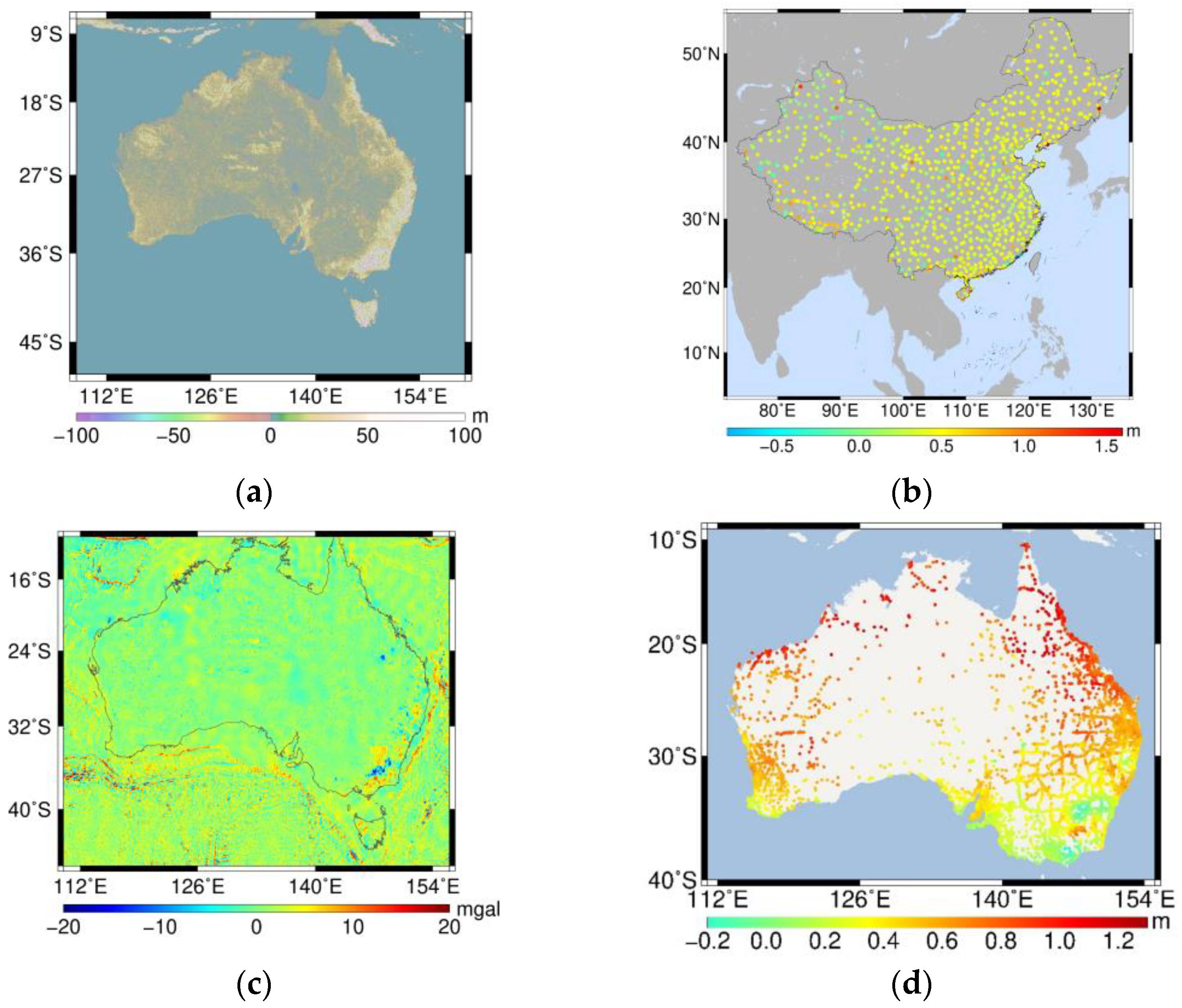
4.3. Determination of the Australian Height Datum Parameters Based on the Geodetic Boundary Value Problem Approach

The combined GNSS/leveling data, gravity anomaly data and GBVP approach could calculate the AHD parameters. The vertical offset is related to the deviation between the geometric geoid and the gravimetric geoid. The gravimetric geoid can be determined based on the RCR technique. In this technique, EIGEN-6C4 and the RTM provide the long and short wavelength parts of the gravity field spectrum, and the residual gravity field spectrum is provided by the residual gravity anomaly. We used $1^{\prime }\times 1^{\prime }$ Shuttle Radar Topographic Mission (SRTM) data and the topographic reference model to build the RTM. The topographic reference model adopts DTM2006 [36]. The distribution of residual terrain model elevations in Australia is shown in Figure 4b.

The RTM and forward-modeling gravitational potential formulas for prisms were used to calculate the RTM geoid height and the RTM gravity anomaly, and the radius of integration was 2 degrees [33,36]. Combining the RTM gravity anomaly, GGM gravity anomaly and free-air gravity anomaly data allowed for determining the residual gravity anomaly. The distribution of the residual gravity anomaly in Australia is shown in Figure 4c.

Stokes integration with the residual gravity anomalies can determine the residual geoid height. We used EIGEN-6C4 to calculate the GGM geoid height and used GNSS/leveling data to calculate the geometric geoid height. Combining the GGM geoid height, geometric geoid height, residual geoid height and RTM geoid height allowed for determining the vertical offset of the Australian height datum relative to the global vertical datum $W_0$. Figure 4d shows the vertical offsets of the AHD calculated using GNSS/leveling data.

The vertical offsets of the AHD include an obvious inclination phenomenon in the north–south direction. Systematic errors in the result were absorbed using a parametric model, and the parameter results of the parametric model are shown in Table 7. The vertical offset of the AHD relative to the global vertical datum W₀ was 0.4885 m, and the geopotential value of the Australian Height Datum was 62,636,851.935 m²s⁻².

5. Conclusions

The unification of the global vertical datum has been an important problem to be solved in geodesy for a long time. The main goal for unifying the global vertical datum system is to determine the geopotential value W₀ of the geoid and to calculate the vertical offset between the local vertical datum and the global vertical datum W₀.

First, we combined GMSS data and the EIGEN-6C4 model to determine the geopotential value W₀. The GMSS data were obtained based on multi-star altimetry data from the past 24 years. After collinear adjustment and crossover adjustment, the intersection mismatch of altimetry data was reduced to millimeters. The GMSS data accuracy was evaluated using the CLS15, DTU18 and SDUST2020 models, and the result showed that the GMSS data accuracy was reliable. As the result, the geopotential value W₀ was 62,636,856.82 m²s⁻².

Using the unified vertical datum method allowed for determining the vertical offset of the local elevation datums relative to the global vertical datum W₀ identified in this study. We evaluated the vertical datum parameters of the Australian height datum using the GBVP approach, and the Chinese height datum using the geopotential difference approach. The GBVP approach utilized the remove–compute–restore (RCR) technique to recover high-frequency gravity signals, which can compensate for the omission error of the GGM. As a result of the GBVP solution, the geopotential value of the AHD was 62,636,851.935 m²s⁻², and the vertical offset of the AHD relative to the global vertical datum W₀ was 0.4885 m. As a result of the geopotential difference approach, the geopotential value of the Chinese height datum was 62,636,861.412 m²s⁻², and the vertical offset of the Chinese height datum was −0.4592 m.

References

1. Hayden, T. Geopotential of the Geoid-Based North American Vertical Datum. Master’s Thesis, Graduate Studies, University of Calgary, Calgary, AB, Canada, 2013. [Google Scholar]
2. Zhang, C. The role of global vertical benchmarks in global change research. Geosci. Front. 2002, 9, 393–400. [Google Scholar]
3. Zhang, L.; Li, F.; Chen, W.; Zhang, C. Height datum unification between Shenzhen and Hong Kong using the solution of the linearized fixed-gravimetric boundary value problem. J. Geod. 2009, 83, 411–417. [Google Scholar] [CrossRef]
4. Li, J.; Chu, Y.; Xu, X. Determination of regional and global elevation datum differences. J. Surv. Mapp. 2017, 46, 12. [Google Scholar]
5. Meyer, T.H.; Roman, D.R.; Zilkoski, D.B. What does height really mean? Part III: Height Systems. Surv. Land Inf. Sci. 2006, 66, 149–160. [Google Scholar]
6. Gauss, C.F. Bestimmung des Breitenunterschiedes Zwischen den Sternwarten von Göttingen und Altona: Durch Beobachtungen am Ramsdenschen Zenithsector; Bei Vandenhoeck und Ruprecht: Göttingen, Germany, 1828. [Google Scholar]
7. Chen, J.; Tapley, B.; Save, H.; Tamisiea, M.E.; Bettadpur, S.; Ries, J. Quantification of ocean mass change using gravity recovery and climate experiment, satellite altimeter, and Argo floats observations. J. Geophys. Res. Solid Earth 2018, 123, 10,212–10,215. [Google Scholar] [CrossRef]
8. Sánchez, L.; Čunderlík, R.; Mikula, K.; Minarechová, Z.; Dayoub, N.; Šíma, Z.; Vatrt, V.; Vojtíšková, M. A conventional value for the geoid reference potential W0. In Proceedings of the Unified Analysis Workshop, Paris, France, 10–12 July 2017. [Google Scholar]
9. Sanchez, L. Definition and realisation of the SIRGAS vertical reference system within a globally unified height system. In Proceedings of the Dynamic Planet, Cairns, Australia, 22–26 August 2005; pp. 638–645. [Google Scholar]
10. Amin, H.; Sjöberg, L.E.; Bagherbandi, M. A global vertical datum defined by the conventional geoid potential and the Earth ellipsoid parameters. J. Geod. 2019, 93, 1943–1961. [Google Scholar] [CrossRef]
11. Yuan, J.; Guo, J.; Zhu, C.; Li, Z.; Liu, X.; Gao, J. SDUST2020 MSS: A global 1′ × 1′ mean sea surface model determined from multi-satellite altimetry data. Earth Syst. Sci. Data Discuss. 2022, 15, 155–169. [Google Scholar] [CrossRef]
12. Schaeffer, P.; Faugére, Y.; Legeais, J.; Ollivier, A.; Guinle, T.; Picot, N. The CNES_CLS11 global mean sea surface computed from 16 years of satellite altimeter data. Mar. Geod. 2012, 35, 3–19. [Google Scholar] [CrossRef]
13. Jin, T.; Li, J.; Jiang, W. The global mean sea surface model WHU2013. Geod. Geodyn. 2016, 7, 202–209. [Google Scholar] [CrossRef]
14. Chu, Y.; Li, J. Combine the global gravity field model and the sea surface height model to determine the mean sea surface position constant. Geod. Geodyn. 2012, 32, 5. [Google Scholar]
15. Dayoub, N.; Edwards, S.J.; Moore, P. The Gauss–Listing geopotential value W0 and its rate from altimetric mean sea level and GRACE. J. Geod. 2012, 86, 681–694. [Google Scholar] [CrossRef]
16. Yuan, J.; Guo, J.; Liu, X.; Zhu, C.; Niu, Y.; Li, Z.; Ji, B.; Ouyang, Y. Mean sea surface model over China seas and its adjacent ocean established with the 19-year moving average method from multi-satellite altimeter data. Cont. Shelf Res. 2020, 192, 104009. [Google Scholar] [CrossRef]
17. Burša, M.; Kenyon, S.; Kouba, J.; Raděj, K.; Šíma, Z.; Vatrt, V.; Vojtíšková, M. Dimension of the Earth’s general ellipsoid. Earth Moon Planets 2002, 91, 31–41. [Google Scholar] [CrossRef]
18. Bao, L.; Peng, G.; Peng, H.; Jia, Y.; Qi, G. First accuracy assessment of the HY-2A altimeter sea surface height observations: Cross-calibration results. Adv. Space Res. 2015, 55, 90–105. [Google Scholar] [CrossRef]
19. Beckley, B.D.; Zelensky, N.P.; Holmes, S.A.; Holmes, S.A. Assessment of the Jason-2 extension to the TOPEX/Poseidon, Jason-1 sea-surface height time series for global mean sea level monitoring. Mar. Geod. 2010, 33, 447–471. [Google Scholar] [CrossRef]
20. Liu, Z.; Yang, J.; Zhang, J.; Cui, W. Global data quality assessment based on Jason-3 satellite altimeter alignment with Jason-2 data. Acta Oceanol. Sin. 2020, 42, 11. [Google Scholar]
21. Andersen, O.; Knudsen, P.; Stenseng, L. A new DTU18 MSS mean sea surface–Improvement from SAR altimetry. In Proceedings of the 25 Years of Progress in Radar Altimetry Symposium, Ponta Delgada, Portugal, 24–29 September 2018. [Google Scholar]
22. CNES. Along-Track Level-2+ (L2P) SLA Product Handbook. Available online: https://www.aviso.altimetry.fr/fileadmin/documents/data/tools/hdbk_L2P_all_missions_except_S3.pdf (accessed on 25 November 2022).
23. Ebadi, A.; Ardalan, A.A.; Karimi, R. The Iranian height datum offset from the GBVP solution and spirit-leveling/gravimetry data. J. Geod. 2019, 93, 1207–1225. [Google Scholar] [CrossRef]
24. Gerlach, C.; Rummel, R. Global height system unification with GOCE: A simulation study on the indirect bias term in the GBVP approach. J. Geod. 2013, 87, 57–67. [Google Scholar] [CrossRef]
25. Vu, D.T.; Bruinsma, S.; Bonvalot, S.; Bui, L.K.; Balmino, G. Determination of the geopotential value on the permanent GNSS stations in Vietnam based on the Geodetic Boundary Value Problem approach. Geophys. J. Int. 2021, 226, 1206–1219. [Google Scholar] [CrossRef]
26. Andersen, O.B.; Knudsen, P. DNSC08 mean sea surface and mean dynamic topography models. J. Geophys. Res. Ocean. 2009, 114. [Google Scholar] [CrossRef]
27. Yuan, J.; Guo, J.; Zhu, C.; Hwang, C.; Yu, D.; Sun, M.; Mu, D. High-resolution sea level change around China seas revealed through multi-satellite altimeter data. Int. J. Appl. Earth Obs. Geoinf. 2021, 102, 102433. [Google Scholar] [CrossRef]
28. Sanchez, B.V.; Pavlis, N.K. Estimation of main tidal constituents from TOPEX altimetry using a Proudman function expansion. J. Geophys. Res. Ocean. 1995, 100, 25229–25248. [Google Scholar] [CrossRef]
29. Huang, M.; Wang, R.; Chai, G.; Ouyang, Y. Multi-generation satellite altimetry data combined adjustment and gravity field inversion. J. Wuhan Univ. (Inf. Sci. Ed.) 2007, 11, 988–993. [Google Scholar]
30. Wagner, C.A. Radial variations of a satellite orbit due to gravitational errors: Implications for satellite altimetry. J. Geophys. Res. Solid Earth 1985, 90, 3027–3036. [Google Scholar] [CrossRef]
31. Rummel, R. Principle of satellite altimetry and elimination of radial orbit errors. In Satellite Altimetry in Geodesy and Oceanography; Rummel, R., Sansò, F., Eds.; Springer: Berlin/Heidelberg, Germany, 1993; pp. 190–241. [Google Scholar]
32. Jin, T.; Li, J.; Xing, L.; Chu, Y. Unified study of multi-source satellite altimetry data benchmark. Geod. Geodyn. 2008, 28, 5. [Google Scholar]
33. Zhang, P.; Bao, L.; Guo, D.; Wu, L.; Li, Q.; Liu, H.; Xue, Z.; Li, Z. Estimation of vertical datum parameters using the GBVP approach based on the combined global geopotential models. Remote Sens. 2020, 12, 4137. [Google Scholar] [CrossRef]
34. Nagy, D.; Papp, G.; Benedek, J. Corrections to “The gravitational potential and its derivatives for the prism”. J. Geod. 2002, 76, 475. [Google Scholar] [CrossRef]
35. Nagy, D.; Papp, G.; Benedek, J. The gravitational potential and its derivatives for the prism. J. Geod. 2000, 74, 552–560. [Google Scholar] [CrossRef]
36. Hirt, C.; Featherstone, W.; Marti, U. Combining EGM2008 and SRTM/DTM2006. 0 residual terrain model data to improve quasigeoid computations in mountainous areas devoid of gravity data. J. Geod. 2010, 84, 557–567. [Google Scholar] [CrossRef]
37. Zhang, P.; Li, Z.; Bao, L.; Zhang, P.; Wang, Y.; Wu, L.; Wang, Y. The Refined Gravity Field Models for Height System Unification in China. Remote Sens. 2022, 14, 1437. [Google Scholar] [CrossRef]
38. Beckley, B.D.; Zelensky, N.P.; Luthcke, S.B.; Luthcke, S.B. Towards a seamless transition from TOPEX/Poseidon to Jason-1. Mar. Geod. 2004, 27, 373–389. [Google Scholar] [CrossRef]
39. Sánchez, L.; Čunderlík, R.; Dayoub, N.; Mikula, K.; Minarechová, Z.; Šíma, Z.; Vatrt, V.; Vojtíšková, M. A conventional value for the geoid reference potential W0. J. Geod. 2016, 90, 815–835. [Google Scholar] [CrossRef]
40. Petit, G.; Luzum, B. IERS 2010 conventions. In IERS Technical Note; Bundesamt für Kartographie und Geodäasie: Frankfurt, Germany, 2010; p. 179. [Google Scholar]
41. Čunderlík, R.; Mikula, K. Numerical solution of the fixed altimetry-gravimetry BVP using the direct BEM formulation. In the Observing Our Changing Earth; Sideris, M.G., Ed.; Springer: Berlin/Heidelberg, Germany, 2009; Volume 133, pp. 229–236. [Google Scholar]
42. Burša, M.; Kenyon, S.; Kouba, J.; Šíma, Z.; Vatrt, V.; Vítek, V.; Vojtíšková, M. The geopotential value W 0 for specifying the relativistic atomic time scale and a global vertical reference system. J. Geod. 2007, 81, 103–110. [Google Scholar] [CrossRef]
43. Burša, M.; Kouba, J.; Raděj, K.; True, S.A.; Vatrt, V.; Vojtíšková, M. Monitoring geoidal potential on the basis of TOPEX/POSEIDON altimeter data and EGM96. In Geodesy on the Move; Springer: Berlin/Heidelberg, Germany, 1998; pp. 352–358. [Google Scholar]
44. Rapp, R. Equatorial radius estimates from Topex altimeter data. In Festschrift to E; Groten, M., Becker, G., Hein, R.R., Eds.; Institute of Geodesy and Navigation, Univ. FAF: Munich, Germany, 1995. [Google Scholar]
Figure 1. Distribution of the GNSS/leveling data in (a) China and (b) Australia. (c) Distribution of the gridded free-air gravity anomaly in Australia.
Remotesensing 15 00912 g001
Figure 2. Process used to calculate the geoid potential constant W0 by using altimetry data.
Remotesensing 15 00912 g002
Figure 3. Mean sea surface model in the oceanic region.
Remotesensing 15 00912 g003
Figure 4. (a) The distribution of the vertical offsets of the Chinese height datum relative to the global vertical datum at the GNSS/leveling data points. (b) Distribution of the residual terrain model elevations in Australia. (c) Distribution of residual gravity anomaly in Australia. (d) The distribution of the vertical offsets of the Australian height datum relative to the global vertical datum at the GNSS/leveling data points.
Remotesensing 15 00912 g004