Article

Determination of Accurate Dynamic Topography for the Baltic Sea Using Satellite Altimetry and a Marine Geoid Model

by
Majid Mostafavi
1,*,
Nicole Delpeche-Ellmann
2,
Artu Ellmann
1 and
Vahidreza Jahanmard
1
1
Department of Civil Engineering and Architecture, Tallinn University of Technology, 19086 Tallinn, Estonia
2
Department of Cybernetics, School of Science, Tallinn University of Technology, 19086 Tallinn, Estonia
*
Author to whom correspondence should be addressed.
Remote Sens. 2023, 15(8), 2189; https://doi.org/10.3390/rs15082189
Submission received: 24 March 2023 / Revised: 13 April 2023 / Accepted: 17 April 2023 / Published: 20 April 2023
(This article belongs to the Special Issue Satellite Altimetry: Technology and Application in Geodesy)

Abstract

:
Accurate determination of dynamic topography (DT) is expected to quantify a realistic sea surface with respect to its vertical datum and in identifying sub-mesoscale features of ocean dynamics. This study explores a method that derives DT by using satellite altimetry (SA) in conjunction with a high-resolution marine geoid model. To assess the method, DT was computed using along-track SA from Sentinel- 3A (S3A), Sentinel-3B (S3B), and Jason-3 (JA3), then compared with DT derived from a tide-gauge-corrected hydrodynamic model (HDM) for the period 2017–2019 over the Baltic Sea. Comparison of SA-derived DT and corrected HDM showed average discrepancies in the range of ±20 cm, with root mean square errors of 9 cm (for S3B) and 6 cm (for S3A and JA6) and a standard deviation between 2 and 16 cm. Inter-comparisons between data sources and multi-mission SA over the Baltic Sea also potentially identified certain persistent and semi-persistent problematic areas that are either associated with deficiencies in the geoid, tide gauge, HDM, and SA or a combination of all of these. In addition, it was observed that SA data have the potential to show a more realistic (detailed) variation of DT compared to HDM, which tended to generate only a smooth (low-pass) surface and underestimate DT.

1. Introduction

Accurate and consistent absolute sea level determination is a fundamental indicator of changes in our climate and is applicable in many research disciplines, including hydrogeodesy and oceanography. It is well known that sea level can be deduced from different sources, including tide gauge (TG) stations, hydrodynamic models (HDMs), and satellite altimetry (SA) [1]. These data sources, whilst capable, often refer to different vertical datums with different spatio-temporal resolutions [1]. For instance, for SA derived sea surface heights (SSH), the vertical reference is the ellipsoid, whereas TG data may refer to a geoid (equipotential surface of the earth) or mean sea level (MSL), and the vertical datum of HDM can often be undisclosed (Figure 1) and generally may have a bias that varies both spatially and temporally with respect to the records of nearby TG stations [1,2]. These differences often make it challenging for comparison and consistency among the sources. Consequently, this hinders the full understanding of continuous sea level variations from coast to offshore.
Instead, a useful component that reasonably represents sea level dynamics, capturing both mean and sub-mesoscale dynamics (i.e., <10 km ocean features), is dynamic topography (DT), which dynamically varies in a spatio-temporal domain in intricate patterns [3]. DT can be derived using two methods. Firstly, via an oceanographic approach, DT is calculated by using sea level data from ocean models. However, in many cases, the vertical datum often is unknown or undisclosed. Secondly, DT is calculated by using the difference between the SA-determined SSH and a suitable geoid model (i.e., DT = SSH-geoid). Note that DT is a more realistic component than the sea level anomaly (SLA = SSH-MSL). Instead of mean sea level (MSL), using a geoid allows for the determining of both mean and time-varying dynamics that exist so that sub-mesoscale dynamics can potentially be determined. Thus, the main intention of this study is to describe in detail a methodology that computes DT obtained from SA. A secondary aspect that this study examines is a quantitative comparison of the differences between the DT obtained from SA and the TG corrected HDM (i.e., biases accounted for) and a provisional investigation into the causes of these differences.
Even though multiple global geoid models are available (such as the Earth Gravitational Model EGM08 [4]), they are not sufficient in terms of accuracy and spatial resolution. For DT to make a difference, one requires the utilization of high-resolution regional geoid models [1,5] that can be obtained by in situ gravity and remote sensing measurements (using SA-derived gravity data products and ship- or airborne gravity measurements) along with robust and intricate modeling techniques [6]. Most study areas are limited in developing high-resolution geoid models due to a lack of vital technical expertise and equipment (which can be expensive). Many countries, however, are moving forward in computing accurate geoid models for their land–sea areas (e.g., the Baltic Sea region, Canada, Australia, etc.). An example is illustrated with respect to the Baltic Sea countries of pursuing a collaboration amongst nations, which has now resulted in a regionally calculated high-resolution geoid model (NKG2015) [6]. This effort now paves the way for further developments in marine studies that were not possible before.
Historically, TG stations provide a reliable measurement of relative sea level, i.e., relative to land-bound benchmarks. However, in some areas (such as the Baltic Sea region) it is necessary for TG records to be corrected for vertical land motion (VLM) to acquire absolute sea level (i.e., refer to the Earth’s center of mass) [7]. In addition, the major limitation of TG observations is that they are not representative for offshore sea level variability. Meanwhile, SA and HDM data are quite capable of representing absolute sea level both in coastal and offshore areas; once a HDM is corrected for the bias and tilts that exist, a realistic comparison with other sources is possible. Note that HDM compilations are based on mathematical models whereas the actual marine areas are unpredictable and turbulent. Thus, it is expected that the comparison of SA (which remotely measures the real sea surface) with corrected HDM (which is the only available source of DT offshore) can reveal the actual sea surface topography and possible modeling imperfections. In addition, the present study hints at problematic issues either with the geoid, HDM, TG, or SA datasets. Recently developed high-resolution regional HDMs can reproduce the best spatio-temporal resolution sea level variations nearshore and offshore. Therefore, it will be more effective to use SA data in conjunction with HDM to validate the retrieval of accurate absolute sea level variations offshore, with TG data providing realistic quality control at the coast [8,9].
The perspective undertaken in this study is to show that SA-derived DT can be accurately calculated both at the coast and offshore. It should be noted that SA data have some limitations, especially in coastal areas and sub-arctic sea ice regions. The SA data are affected by the vicinity to the coast of a few kilometers, where the radar echo interacts with the nearby land surface, leading to corrupted waveforms [10]. Moreover, SA data are aligned to the International Terrestrial Reference Frame (ITRF), which may not necessarily coincide with the reference frame of the coordinates of land-bounded TG stations. TG stations normally refer to other pan-continental or national reference datums, such as the European Terrestrial Reference System (ETRS) and its national realizations. Another difficulty is related to the tidal effects and altimeter observation corrections (including geophysical and media corrections) that often become inaccurate close to the coast [11]. Furthermore, seasonal sea ice coverage, irregular coastlines, and the presence of numerous archipelagos, small islands, and rocks within 10 km from the coastline would affect SA data quality in many areas [10,12,13,14,15,16].
The potential of SA for monitoring coastal sea level variations and many oceanographic fields has motivated the development of coastal altimetry studies. Hence, several projects (e.g., PISTACH [17]; PEACHI [18]; COASTALT [19]; X-TRACK [20], Baltic+SEAL [21]) have been developed to improve the retrieval of sea level parameters from coastal waveforms of SA. In particular, the European Space Agency’s Baltic+ Sea Level (ESA Baltic+SEAL) Project, launched in April 2019, is generating enhanced multi-mission sea level products that are specifically developed for the Baltic Sea. To attain a consistent description of sea level variability, a new re-tracking algorithm was developed and applied. This yields a homogeneous SSH determination that is particularly adapted for the complex areas of the Baltic Sea and North Sea, especially with respect to the presence of seasonal sea ice and complex coastal geomorphology [21].
As mentioned earlier, the focus of this study is to explore a developed methodology to estimate accurate DT in the Baltic Sea using a synergy of SA, corrected HDM, a dense TG network, and a high-resolution geoid model. The Baltic Sea is a semi-enclosed shallow sea in northern Europe that is heavily influenced by a massive density of marine traffic, coastal activities, port development, and sub-mesoscale marine dynamics [10]. Thus, knowledge of accurate DT variations in the Baltic Sea is critical for many reasons (e.g., consistency amongst data sources, sea level trends estimate, derivation of currents, etc.). In addition, since no sea level source is perfect (mentioned above with respect to the limitation of HDM and SA), but given that they all refer to the same vertical datum, this now allows a logical inter-comparison to be performed. By performing statistical analysis, this comparison has the potential to identify the problematic areas of the sea level sources utilized. Note that the sources of these problematic areas are only provisionally explored in this study to demonstrate the usefulness of DT and the benefits that the synergy of different sources of sea level data can indirectly reveal. For a more detailed understanding of these sources, more resources are required that are out of the scope of this study but can be pursued for future studies. Note that the other sources of sea level from which DT can also be derived consist of shipborne GNSSs (global navigation satellite systems) and airborne laser scanning profiles. For instance, Ref [22] used airborne laser scanning profiles for determining DT. In addition, Ref [23,24] used shipborne GNSS profiles for determining DT over the Baltic Sea. Usage of these other sources are, however, restricted by their spatial and temporal resolution.
The method developed and described in this study was possible for the Baltic Sea region, which is fortunate to have a dense multi-national TG network, a high-resolution geoid model, a land uplift model, and access to data-assimilated HDM and SA data specifically tuned to the sea conditions. In particular, HDM bias with respect to the TG readings has been eliminated along the SA track, so the corrected HDM provides accurate DT estimates both near- and offshore. Such a combination can assist in retrieving accurate DT from relatively short altimetry time series [25]. This method to our knowledge has not been performed before, especially from the point of view of utilizing multi-mission along-track SA data and a high-resolution geoid model. It also can be applied to other sea areas.
Previous studies have examined the performance of SA data in the Baltic Sea [10,12,13,14,15,16,26,27,28], but these studies mostly examined the sea surface in terms of SSH and were limited to mostly validation of SA data. In addition, many of these studies examined only a section of the Baltic Sea.
Thus, the focus of this study is (i) development and demonstration of a detailed method for determining accurate DT using along-track SA, derived for multiple satellite missions in the entire Baltic Sea, and (ii) by statistically and qualitatively comparing the discrepancy between SA and corrected HDM to identify the persistent and semi-persistent patterns that could potentially reveal problematic areas of the various sources utilized (e.g., geoid model, TG, HDM, and SA). The time period examined for all data sources was between 2017 and 2019; this was based on the availability of all the data sources, since the SA data were sourced from the Baltic+SEAL project and these data were up to 2019 (at the time of the study). This three-year long-term period, however, is considered to be representative enough for our objectives to describe the method and to show its potential.
This paper is organized in a format such that the developed methodology is described in Section 2 and the study area and utilized datasets are described in Section 3. Section 4 presents the results of the obtainable DT accuracy and identifies the areas with persistent and semi-persistent patterns by comparing the different sources of sea level data and multi-mission SA. The results of this study are discussed in Section 5, whereas Section 6 contains a brief summary of this study.

2. Methodology

This section describes the method employed to achieve accurate DT using two approaches: the first approach utilizes HDM, and the second approach uses SA. The first approach involves extracting the HDM data points that coincide with the SA along-track data points. Once this is performed, the HDM data points are corrected via TG observations by means of utilizing virtual stations (Section 2.1). The second approach requires a geoid model and some other vital auxiliary corrections for obtaining DT from the SA-computed sea surface heights (Section 2.2). This original HDM provides high-correlation estimates of TG-observed sea levels along the Baltic coastline. However, the original HDM also contains some biases due to the undisclosed actual vertical datum used [2]. Hence, for further computational steps, it is vital to retrieve reliable DT values in a stable vertical reference datum by correcting the HDM. For this purpose, the HDM correction method with respect to the TG observations by means of utilizing virtual stations (VS) was applied (cf. Section 2.1), to consider these biases as well as unify the vertical reference of the HDM to the same reference surface as the TG and SA data. The second approach requires a geoid model and some other vital auxiliary corrections for obtaining DT from the SA-computed sea surface heights (Section 2.2). The difference between SA-derived DT ( D T S A ) and HDM-derived DT ( D T H D M ) is then calculated both spatially and temporally using VSs. It is expected that the HDM may appear to be somewhat insensitive in terms of fully capturing the short-wavelength marine surface variations; this is mainly due to the fact that it is a model with limitations (e.g., parametrization, approximations model forcings, etc.). The HDM, however, is still a key source because it is capable of simulating both coastal and offshore sea level data. The assumption in the present study is that once the HDM is corrected for this bias and tilts, it can be compared to the SA data. Utilization of the geoid allows the comparison of the corrected HDM and SA to be performed; otherwise, the two datasets would be incomparable in an absolute sense.
In this study, it was essential that the HDM was corrected and considered as the ground truth during examination of the D T S A estimates. Note, however, that in the comparisons, one of the sources had to be assumed to be the ground truth (in this case the corrected HDM via TGs) to obtain the discrepancies. So, the comparison of appropriately corrected HDM (which was always the case in the further comparisons) versus D T S A provides a good quantification of the accuracy of the latter.

2.1. TG/HDM Based DT Estimates

2.1.1. General Overview of the Method

This section describes the method used to correct the HDM derived DT ( D T H D M ) at specific locations that are referred to as virtual stations (VSs). The concept of utilizing VSs originates from the following characteristics: (i) it is important that D T H D M be calculated at the same data points as SA (i.e., in space and time); (ii) correction of HDM is assumed to be more accurate at VSs rather than at the near-shore location of TGs, and (iii) the study area is equipped with numerous TGs that may lie in proximity to SA data points.
It is commonly known that TG records are valid nearshore and may not adequately represent offshore DT. Instead, a regional HDM is an independent data source that can provide sea level data both at the coast and offshore. The method proposed is that by calculating the relative difference between DTs of HDM at the location of a TG and the location of the proposed VS, it is possible to calculate the DT at the VS via the TG’s readings. This is performed by simply adding this relative difference in DTs (Equations (1)–(3)). Different interpolation methods (linear interpolation, thin plate spline regression, and inverse distance weighted (IDW)) were explored in [2] and the results show a difference of around 2 cm. However, the IDW showed slightly more realistic results, so in this study, a similar procedure was implemented.
In addition, the vertical reference datum of HDM is often unknown/undisclosed and may contain some errors and discrepancies from the exact reality of sea level. To overcome such limitations, a bias correction solution needs to be introduced to correct the HDM by a one-dimensional vertical shift at a single time instant (which changes during the time of the SA cycle). This correction represents the difference between the TG and the HDM data at a VS. The correction values (i.e., bias) change over time, and we computed this correction at the time of SA. The reason why it changes is due to two components: (i) The fact that the TG measures in situ data (i.e., the actual situation) whilst the HDM is based on a mathematical model that attempts to model the sea surface based on the input forces, models, etc. So, it is expected that the HDM may have an error when compared to reality. (ii) The HDM vertical reference is often undisclosed and can vary both spatially and temporally. Basically, the error between the HDM and the tide gauges can be separated into two parts: constant and time-variable. For simplicity, we express the “HDM bias” as a combination of all errors. In Ref. [2], a detailed examination was made into the bias and the study showed that the HDM bias can be spatially interpolated at each time instant in order to correct the HDM, and since the bias was interpolated (not the sea level), IDW interpolation can be a good choice. This bias correction method between a TG and HDM at a VS is explained in more detail below in Equations (1)–(5) for each SA cycle. Note that in the used equations, the HDM correction values (Equation (5)) are both time- and location-dependent.

2.1.2. Detailed Method

Determination of the VS locations is the first step of HDM correction. A VS is selected as the closest location of a good-quality SA data point approaching the coastline (Figure 1). Each SA track has at least two VSs (at the beginning and the end of the track), though many tracks have more along-track VSs, close-to-coast, and nearby TG stations (cf. Figure 2a).
Note that the coastline-located TGs may not exactly coincide with the HDM data grid nodes. In addition, the available HDM data near TG locations are expected to have some errors due to the limitations of HDM in nearshore and shallow waters. In addition, given the dense network of TG stations in the study area, the TG-derived DT may be valid toward offshore within a valid domain (including the VS’s location) using adjacent TGs and by adding the relative DT, i.e., the difference in DT at the HDM location of the VS and the location of the TG (cf. Figure 2b). In such cases, the DT of the VS is determined using inverse distance weighted (IDW) interpolation slightly seaward at the VS locations. Hence, VS is assumed to represent an enhanced duplicate of the TGs and is consistent with HDM data.
A VS intends to represent the k-nearest TG stations at a SA pass. The nearest TG (hourly, t) readings are interpolated (interp) linearly at the time of SA overfly cycle time ( t c y c l e ), whereas the relative DT ( D T R e l a t i v e ) is added to this to retrieve DT at the location of the VS ( D T T G @ V S ). The D T R e l a t i v e is the difference between the HDM-based DT at the location of the VS ( D T H D M φ V S , λ V S , t c y c l e and that at the location of the TG ( D T H D M φ T G , λ T G , t c y c l e ). The D T R e l a t i v e could provide more realistic DT of TG readings at the location of the VS rather than simple interpolation (cf. Figure 2b) since the assumption is that the HDM is providing a reference base surface sea level, not a precise one. By adding the D T R e l a t i v e to the timewise-interpolated D T T G   i n t e r p D T T G φ j , λ j , t c y c l e , the D T V S is obtainable. The adjacent D T T G @ V S (Figure 2b red triangle) to the VS are averaged using IDW [29] to yield the DT at the VS location ( D T V S φ V S , λ V S ), which now can be used to determine the bias of the HDM.
  D T T G @ V S φ j , λ j , t c y c l e = i n t e r p D T T G φ j , λ j , t c y c l e + D T R e l a t i v e φ j , λ j , t c y c l e
where
D T R e l a t i v e φ j , λ j , t c y c l e = i n t e r p [ D T H D M φ V S , λ V S , t c y c l e D T H D M φ T G , λ T G , t c y c l e ]
and
D T V S φ V S , λ V S , t c y c l e = 1 j = 1 k p j j = 1 k p j   .   D T T G @ V S φ j , λ j , t c y c l e    
Note that k is the total number of available TG stations reasonably close to the VS. Hence, a 130 km radius was selected based on empirical experience in the study area to guarantee the availability of at least one TG station within this radius and exclude farther TGs. The symbol p j is the assigned IDW weight for the j-th TG station with coordinates φ j , λ j , which is computed as follows:
p j = c 0 d i s t j  
where c 0 is the minimum distance of the associated TGs to the VS and d i s t j is the distance of the j-th participating TG to the VS. Using the IDW, the TG station with the minimum distance (~3 km) to the VS has the maximum effect on D T V S . In addition, distant TGs would be neglected (TGs exceeding 130 km distance). The D T V S is expected to represent a more truthful condition of the sea level (in contrast to D T T G ) that can be compared to the SA data point. For the SA passes that are near only a single (k = 1) TG at each side of the coast, only one TG reading is selected to obtain the D T V S (i.e., D T V S t c y c l e = i n t e r p ( D T T G t ), interpolated time-wise only) with maximum weight (p = 1).
D T V S is compared with D T H D M to remove any possible bias of the HDM. The HDM bias at the location of each VS ( B i a s H D M V S φ V S , λ V S ) is determined by the difference between D T V S and the initial HDM values D T H D M :
B i a s H D M V S φ V S , λ V S , t c y c l e = D T H D M φ V S , λ V S , t c y c l e D T V S φ v s , λ V S , t c y c l e  
Recall that the assumption made in this study is that the VS tends to represent TG observations and is more or less a reliable ground truth that better reflects nearshore sea dynamics. The B i a s H D M V S represents both vertical reference datum discrepancies and HDM modeling errors. In addition, both HDM and TG data have hourly records, so the D T H D M and D T T G are temporally (and linearly) interpolated at the SA overfly time instant ( t c y c l e ). In addition, since HDM data points spatially do not exactly coincide with SA along-track points ( φ S A , λ S A ), a bilinear interpolation of HDM is applied at the SA data points (including VS location). The B i a s H D M V S is interpolated linearly between a pair of VSs along each SA ground track denoted by i n t e r p ( B i a s H D M V S φ S A , λ S A , t c y c l e ) and then subtracted from the initial D T H D M . As a result, the corrected along-track HDM ( D T H D M c o r r ) is obtained, which now coincides and is simultaneous with SA data locations ( φ S A , λ S A ) at the SA overfly time instant t c y c l e :
D T H D M c o r r φ S A , λ S A , t c y c l e = D T H D M φ S A , λ S A , t c y c l e i n t e r p ( B i a s H D M V S φ S A , λ S A , t c y c l e )  
This along-track D T H D M c o r r is assumed as the “first approximation ground truth” and will be checked against the SA derived DT (Section 2.2).

2.2. Estimation of DT from Satellite Altimetry and Statistical Examinations

The general concept of SA measurement includes the satellite’s altimeter transmitting a pulse of known power toward the sea surface. On interacting with the sea surface, the pulse is then reflected to the altimeter. The two-way travel time is determined, yielding the range of the satellite after applying range correction (including geophysical and media corrections). Given the known SA orbit, SA-derived SSH is then obtainable with respect to the reference ellipsoid (cf. Figure 1).
However, a more realistic reference surface to be employed would be that of a geoid to retrieve the DT. For this purpose, along-track D T S A φ i , λ i is determined by subtracting the geoidal height ( N ) from the S S H S A using the following expression:
D T S A φ i , λ i , t c y c l e = S S H S A φ i , λ i , t c y c l e d h φ i N φ i , λ i  
Since original datasets of different SA missions and geoids may refer to different reference ellipsoids, the ellipsoidal correction d h φ i of each data point is required. The ellipsoidal correction is due to the differences in parameters that are associated with each reference ellipsoid (including semi-major and minor axes, flattening, and eccentricity). By applying d h , both datasets (SA and geoid) will refer to the same reference ellipsoid (see also [10]).
d h φ i = a ´ 1 e ´ 2 1 e ´ 2   s i n 2 φ i a 1 e 2 1 e 2   s i n 2 φ i  
where a and a’ are lengths of the semi-major axes of the participating ellipsoids, e and e’ are their corresponding eccentricity values, and φ i is the latitude of the point of interest. The discrepancies between the D T S A and D T H D M c o r r will be examined statistically. In addition, unqualified SA data points (which could be different for each SA cycle) need to be excluded from further data processing.
Errors and outliers of the SA dataset occur due to many reasons such as land-contaminated areas, extreme sea events (e.g., storms, surges, etc.) and waveform retracking sampling problems [10]. To remove these outliers from each SA track/cycle, a sequential approach for data screening is applied. The steps involved:
  • D T S A 
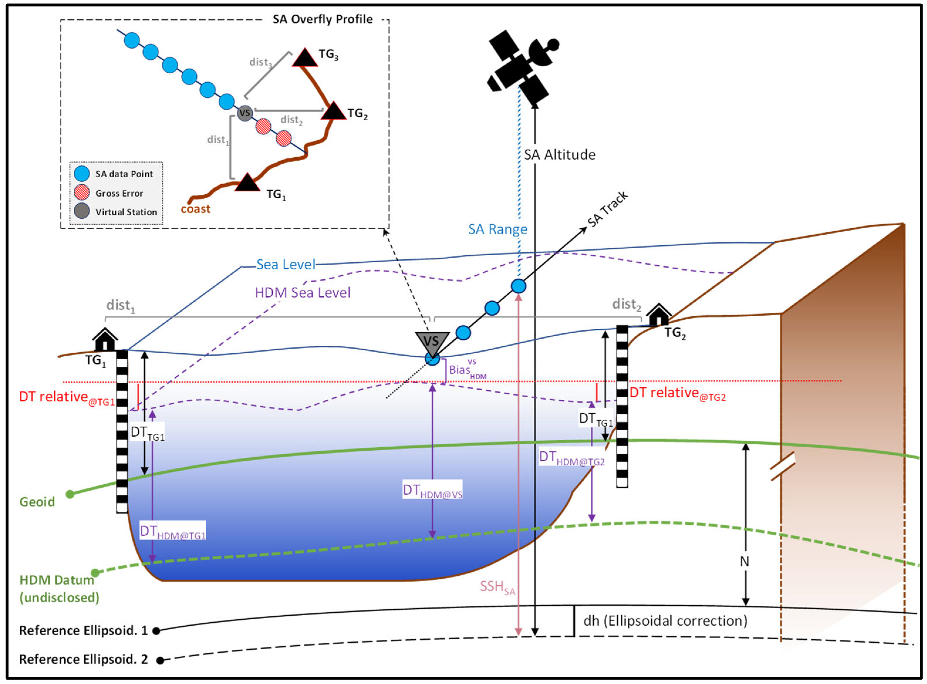
values larger than a specific predefined threshold (| D T S A | > threshold) are considered as gross errors and removed from the data points. This threshold value (here selected as 1.5 m) corresponds to the study area characteristics that depend on historical extrema of the DT occurring in the study area (which is ~1.3 m in the Baltic Sea);
  • The erratic D T S A are identified as those three times larger than the standard deviation (STD) of the mean value of the whole track in a cycle (the longer tracks are divided into sub-tracks to obtain more homogeneous selections);
  • The outliers are detected as elements more than three local scaled moving medians (MADs) from the median D T S A over the 0.5° latitude (~55 km) window length along the track to have a smooth low-pass D T S A behavior.
This approach assists in filtering unqualified data, which allows a more accurate determination of D T S A . After excluding the gross errors and outliers from all SA along-track data points, the remaining good-quality data points (their locations are denoted by sub-index s, e.g., φ s , λ s ) are used for further steps.
The difference between D T S A and D T H D M c o r r is the discrepancy ( Δ D T S A H D M ), which is computed for each footprint point of each participating satellite mission by
Δ D T S A H D M φ s , λ s , t c y c l e = D T S A φ s , λ s , t c y c l e D T H D M c o r r φ s , λ s , t c y c l e
These discrepancies provide a tentative idea of SA agreement to the ground truth within the studied portion of each SA track for each SA mission separately. Statistical analyses of the discrepancies are conducted in terms of the root mean square error (RMSE), standard deviation (STD), and mean of Δ D T S A H D M by the equations below:
M E A N S A H D M   φ s , λ s = 1 m c y c l e = 1 m Δ D T S A H D M φ s , λ s , t c y c l e
S T D S A H D M φ s , λ s = 1 m 1 c y c l e = 1 m Δ D T S A H D M φ s , λ s , t c y c l e M E A N S A H D M φ s , λ s 2
Equations (10) and (11) potentially represent the validation of SA versus the corrected HDM over a single location considering all cycles of the SA mission (minor deviations in data points’ locations from each other at sequential cycles is negligible). The m symbol is the number of qualified SA cycles on each location ( φ s , λ s ). The threshold of m can be selected as 90% of the total number of available cycles of each SA mission during the study period over the study area. The locations ( φ s , λ s ) containing datapoints less than this threshold are excluded. By having the along-track mean of the discrepancies at each location ( M E A N S A H D M   φ s , λ s ), the performance of the individual SA mission over the entire sea (or any selected basin) can be evaluated by:
M E A N S A H D M   m i s s i o n / B a s i n = 1 b s = 1 b M E A N S A H D M φ s   , λ s
S T D S A H D M m i s s i o n / B a s i n = 1 b 1 s = 1 b M E A N S A H D M φ s , λ s M E A N S A H D M   m i s s i o n / B a s i n 2
R M S E m i s s i o n / B a s i n = 1 b s = 1 b M E A N S A H D M   φ s , λ s 2
where b is the total number of ( φ s , λ s ) locations (along-track locations of all passes, separately for each SA mission).
Equations (12)–(14) provide statistics for each SA mission. The RMSE and STD are commonly used to examine both along-track and mission/basin SA data quality. They provide statistically meaningful estimates of D T S A accuracy at a given location or the whole basin via different SA missions. Different SA missions’ data were not merged in this study; therefore, the range of m varies for each mission. The particulars of the used datasets are explained in Section 3. Figure 3 shows the flowchart of the applied methodology and data processing steps.

3. Study Area and Datasets

3.1. Baltic Sea

The Baltic Sea is the world’s second-largest brackish water body (after the Caspian Sea) that has limited water exchange with the North Sea via narrow and shallow Danish straits. This estuarine-type water body’s main source of freshwater originates from the numerous rivers that flow into it. The Baltic Sea is surrounded by nine countries and subdivided into several sub-basins that are based on the geomorphology and bathymetry of the sea area. Due to glacial isostatic adjustment, the Baltic Sea region is also strongly affected by vertical land motion (VLM) [30]. Due to the numerous countries surrounding the Baltic Sea, it has a high density of marine traffic and coastal activities. These attributes make it vital to have a common and realistic vertical datum (e.g., a geoid) that sea level can be referenced against, especially with the marine engineering and navigation activities performed for the Baltic Sea.
Several components based on different time frames affect the sea level dynamics in the Baltic Sea. With respect to the long term, the global sea level change (due to thermal sea water expansion and the melting of glaciers) will influence the Baltic Sea’s level, whilst the variation in temperature, precipitation, and evaporation is expected to mostly exert influence on a decadal time scale [7]. For short-term influences (yearly, seasonally, daily, etc.), variations in the water balance caused by water exchange in the Danish Straits (e.g., saltwater intrusions from the Atlantic (Major Baltic inflow)) that are driven by atmospheric conditions may cause drastic sea level changes. River runoff also affects the water balance, with the biggest freshwater contributor being the Neva River located on the eastern side of the Baltic Sea [31]. It is common in winter months for the Baltic Sea to become ice-covered; the number of sea ice days also changes the dynamics of the sea level [32]. Ice coverage is common in the winter months for the Baltic Sea, especially in the northern (Gulf of Bothnia) and eastern sections (Gulf of Finland). This also has been a challenge for SA in determining the sea surface. However, improved SA coastal retrackers are expected to provide better data products over this region, e.g., Baltic+SEAL [10].
In much shorter time frames (e.g., weekly, daily, and hourly), other localized events also affect the sea level. Most of these events tend to be influenced by meteorological factors [33], especially the winds, which can be strongly anisotropic in the Baltic Sea [34]. However, the dominant wind direction in this area is southwest, but it is common for northerly winds to also be prevalent. Storm surges [35] and coastal upwellings [36] are also quite prevalent in the Baltic Sea, with a more or less seasonal trend. The strongest winds and highest waves are highly expected in the winter and autumn seasons [37]. In addition, temperature and precipitation may contribute to 15–35% of the sea level variability between winter and summer [38]. It is somewhat expected that HDMs may have difficulty reproducing some of these localized events. In addition, the internal Rossby radius can be relatively small, usually within the range of 1–2 km [39]. This makes it very challenging for the numerical models to replicate the (sub)-mesoscale dynamics in this water body. However, with SA, if the satellite flies over at the correct time and its measurement is represented as DT, the SA data may be able to capture some evidence of these small-scale dynamics.

3.2. Datasets

3.2.1. Tide Gauge Stations

The Baltic Sea has one of the world’s densest observational tide gauge networks with remarkably long-term and high-quality local sea level records [40]. Within the study area, 74 TG stations (Figure 4a) were selected to have suitable locations near satellite tracks. The details of each TG station per country can be found in Table 1. An identification number (ID) was assigned to each TG station; the relevant details are given in Appendix A Table A1 as well.
These TG networks are operated by national tide gauge agencies and refer to the corresponding national realization of the EVRS2000 (European Vertical Reference System 2000) vertical datum, the zero level of which is the Normaal Amsterdams Peil (NAP). Hence, all data record vertical datums are harmonized with EVRS2000 using the Baltic Sea Chart Datum 2000 (BSCD2000). In addition, in BSCD2000, land uplift was modeled according to the NKG2016LU model at the epoch 2000.0 [41].
Since TGs measure relative sea level with respect to land, their measurements are required to be corrected for VLM in order to obtain absolute sea level. In the Baltic Sea region, vertical land motion is due to geophysical GIA and varies from -1 mm/year in the Arkona Sea to 10 mm/year in the Gulf of Bothnia [42]. In this study, the land uplift effect was removed from TG observations using the NKG2016LU model. This model includes the latest GIA land uplift model for the Baltic Sea region developed by the Nordic Commission of Geodesy (NKG, www.nordicgeodeticcommission.com, accessed on 26 August 2021). It covers an area from 49° to 75°N and 0° to 50°E [30]. The VLM corrections (from the reference time epoch, i.e., 2000.0) were applied from the model (linearly interpolated at the location of TG) by adding it to the TG readings (to the observation time epoch) [6]. During the selected time span of 2017–2019, some TG hourly data gaps exist, as can be seen in Table 1 and Figure 3b. These gaps were filled using highly correlated adjacent TG stations to reconstruct gap-free TG data, cf. [43]. Figure 5 shows the steps for the TG observation reconstructions. In further steps, TG#33 was excluded from the dataset due to data inconsistency with the other TGs.

3.2.2. Hydrodynamic Model

Nemo-Nordic is a three-dimensional coupled ocean–sea ice model of the Baltic and North Sea based on the NEMO-3.6 (Nucleus for European Modeling of the Ocean) ocean engine, which was developed by the Swedish Meteorological and Hydrological Institutes (SMHI) [44]. In this study, a data-assimilated version (NS01) of the Nemo-Nordic model with an hourly temporal resolution and a spatial resolution of 1 nautical mile (~2 × 2 km) was utilized for the period 2017–2019 (www.smhi.se, accessed on 14 April 2020). The bathymetry of the model was obtained from the General Bathymetric Chart of the Oceans Grid (GEBCO-2014). This HDM provides high-correlation estimates with the TGs along the Baltic coastline. However, this model also contains some errors, which are limited to a standard deviation of around 10 cm due to the undisclosed actual vertical datum used [2]. More details on the possible deficiencies of this particular HDM can be found in [2]. Hence, for further computational steps, it is vital to retrieve reliable DT values in a stable vertical reference datum by applying HDM correction. In this study, the applied methodology to identify and eliminate the above-mentioned HDM errors (for more details see [2]) using geoid-referenced TG-corrected HDM is described, which can be now used for deriving instantaneous and realistic sea level data near- and offshore. Then, the corrected HDM can be used to validate the SA derived DT. For this purpose, the HDM correction method with respect to the TGs was applied (cf. Section 2.1) to consider these biases, as well as unify the vertical reference of the HDM to the same reference surface as for the TG and SA data.
HDM correction (cf. Section 2.1) is basically a shift due to the biased vertical datum of the HDM (with respect to the zero level of the national vertical datum) that can also be due to HDM modeling errors. In this study, the TG was not only used to correct the HDM, but also for examining the discrepancies between HDM data and TG observations at each TG station ( φ T G , λ T G ) using hourly data ( t i ) by:
Δ D T H D M T G φ T G , λ T G , t i = D T H D M φ T G , λ T G , t i D T T G φ T G , λ T G , t i
The mean and standard deviation (STD) of HDM data discrepancies at each TG station (here 73 stations, TG#33 excluded) during the whole study period can be estimated as:
M E A N H D M T G   φ T G , λ T G = 1 y i = 1 y Δ D T H D M T G φ T G , λ T G , t i
S T D H D M T G φ T G , λ T G = 1 y 1 i = 1 y Δ D T H D M T G φ T G , λ T G , t i M E A N H D M T G   φ T G , λ T G 2
where y represents the total number of hourly DT records during 2017–2019 (y = years × days × hours) for Figure 6a or amount of data for each month during 2017–2019 (for Figure 6b). Figure 6 shows the mean and STD of HDM data residuals relative to TG observations during 2017–2019. In the figure, the circle size represents the mean (Equation (16)), whereas the color shows the STD at each TG location over entire Baltic Sea.
From Figure 6b,c, a seasonal pattern of HDM discrepancies is observed. Figure 6c indicates that the maximum discrepancies in the HDM (~30 cm) occur from February to March (winter–spring) and are the smallest during the autumn and summer seasons (less than 20 cm). This could be due to river runoff, snow melting, and other effects (e.g., steric effect) that may not be included in the original HDM (also cf. Section 3.1). Note that for the purpose of this study, the HDM was only corrected at the time instants of the SA cycles. In addition, from Figure 6a, the Swedish TGs (from TG#50 to TG#59) have larger M E A N H D M T G   φ T G , λ T G (~25 cm). This indicates that either the HDMs are overestimating the DT more than usual or that there may be a problem with TG corrections in this part of the study area. Compared to other stations in the Baltic Sea, the Latvian and Estonian TGs (e.g., TG ID 12–19) have the largest S T D H D M T G   (more than 9 cm), as well as some Danish and German TGs (e.g., ID#31, 36, and 37) in Arkona Sea. The TGs with larger S T D H D M T G may indicate problematic issues that require further examination for future studies. For instance, some of these issues could be due to TG data inconsistencies (including the TG zero level).

3.2.3. Geoid Model

The NKG2015 gravimetric quasi-geoid model for the Nordic–Baltic countries was developed by the NKG in 2016 [6]. It is referred to the Geodetic Reference System GRS80 ellipsoid and extends from 53° to 73°N and from 0° to 34°E with a grid spacing 0.01° × 0.02°. The NKG2015 quasi-geoid determination is based on the least-squares modification of Stokes’ formula with additive corrections and using the GOCE/GRACE geopotential model and corrected with a one-parameter fit to the national realizations of the EVRS and has a good agreement with GNSS/levelling control points with a STD of 3.0 cm, whilst the EGM2008 (global model) STD is 4.4 cm [6]. The NKG2015 model was used to retrieve D T S A from satellite derived SSH data (i.e., DT = SSH-geoid). Various studies have estimated the NKG2015 geoid error [24] that could reach up to 15 cm over certain marine areas. Such deficient geoid modeling areas were associated with the poor coverage of marine gravity data. Contrastingly, the global geoid models that are customarily used by the satellite altimetry community are less accurate and with a poorer spatial resolution (typically 0.1° × 0.1°). The availability of such a high-resolution regional geoid model is clearly advantageous for the SA-based DT determination in the present study.

3.2.4. Satellite Altimetry

In this study three satellite missions including Sentinel-3A (S3A), Sentinel-3B (S3B) and Jason-3 (JA3) are examined to determine the DT. These missions have different characteristics (Table 2) and track geometry (Figure 7). S3A and S3B have almost the same track patterns and observed the same place on the Earth within 30 s. The main difference is that S3B orbit flies ±140° out of phase with S3A. In addition, S3A/S3B uses SAR (synthetic aperture radar) mode (by SRAL: Synthetic Aperture Radar Altimeter) whilst JA3 uses LRM (low-resolution mode) over the global ocean (by Poseidon-3B altimeter). The characteristics of the missions are summarized in Table 2.
Recent coastal SA retrackers including ALES+ and ALES+SAR appear to improve the SA data quality [10]. In this study, the ALES+ retracker SA data products for the JA3 data and ALES+SAR for S3A and S3B [21] are used. The difference between ALES+ and ALES+SAR is due to the different signal-to-noise ratios of the SAR mode VS LRM. ALES+ is a modification of ALES (Adaptive Leading-Edge Sub-waveform), which is based on the Brown-Hayne functional form that models the radar returns from the ocean to the satellite. This retracker uses sub-waveforms and adapts the fitting of the signal depending on the sea state also on the slope of its trailing edge [21,45]. Based on ocean and coastal waveform characteristics, it uses leading-edge detection for peaky waveforms. These data are produced by the Baltic+SEAL team project (www.balticseal.eu, accessed on 23 March 2021). The Baltic+SEAL consists of a novel improved multi-mission sea level data product (necessary corrections are applied) for the Baltic Sea, that has been created and validated using the latest innovations in coastal altimetry and data processing. The data products are based on the use of retrackers for both LRM (JA3) and delayed Doppler altimeters (including S3A and S3B) [21].
Compared to the open ocean, SA data are degraded near the shoreline due to land contamination on the radar echo, seasonal sea ice conditions, and corrections effect (e.g., wet tropospheric correction). This yields the altimeter measurements close to the coast (~3 km away) to be flagged as poor data in the Baltic+SEAL dataset. In this study, quality flagging has not been applied in order to assess all available data in the region. Instead, this study applies an iterative data screening approach (cf. Section 2.1) for the removal of the gross errors (| D T S A | > 1.5 m) and outliers (using STD and MAD filters, cf. Section 2.2). However, some other corrections are still needed prior to further investigation to make the SA data compatible with terrestrial data.
SA data in Baltic+SEAL products are not directly compatible with TG data (instantaneous sea level data) as the former dataset is corrected for atmospheric pressure effect using Dynamic Atmosphere Correction (DAC). Since the instantaneous DT is examined in this study, the SA data needs to be de-corrected by adding the DAC back to the SSH before the comparison [27]. In addition, these SA data are referenced to TOPEX/Poseidon (T/P) ellipsoid and ITRF (realization 2008), while the TG observations are referred to NAP and ETRF (European Terrestrial Reference Frame). Also recall that the NKG2015 geoid model refers to the GRS-80 reference ellipsoid. The height difference between the ETRF and ITRF in terms of ellipsoidal heights was applied to the SA data. Moreover, SA data are in the mean tide system while TG readings adopt the zero-tide system [46]. Therefore, the effect of these permanent tide systems is accounted for using [47] conversion into the zero-tide system. In addition, the SA terrestrial reference frame needs to be transferred from ITRF2008 to ETRFYYYY, which is an ETRF realization of the year “YYYY” related to TG observations (in this study: 2017–2019), using the method described by [48]. The aforementioned corrections are necessary to be accounted for to enable using SA data with the modified HDM for retrieving absolute instantaneous DT. These steps are illustrated in Figure 8.
In this study, more than 4 million S3A/3B and JA3 data points (Table 3) along 116 passes during 2017–2019 (131 cycles) were extracted from Baltic+SEAL 20 Hz data products. These SA passes cross 74 nearby TGs; see Table A2 and Table A3 in the Appendix A. The numbers of used TGs are at maximum 16, at minimum 2, and 6 stations on average for Jason-3 tracks and 13, 2, and 6 for Sentinel-3 tracks, respectively (cf. Table A2 in the Appendix A). Table 3 shows the main statistics of these datasets. The SA data points out of the HDM coverage (near the coastline) were excluded (cf. the number of outliers in Table 3) for the consistency of the datasets. The number of locations represents the persistent locations of SA data points in the cycles. The used different SA data periods are also summarized in Table 3. Although the S3B mission was launched in April 2018, the start of usable data is in November 2018. Thus, the S3B data before November 2018 were excluded in this study. Accordingly, in statistical evaluations (by Equations (10)–(12)), 92 cycles of JA3 (whereas the number of qualified cycles m = 82), 33 cycles of S3A (m = 29), and 7 cycles of S3B (m = 6) over 3 years (2017–2019) were investigated.

4. Results

This section presents the statistical results of the method described in Section 2. The main focus is on SA derived DT (from multiple missions) and its evaluation against a corrected HDM both near- and offshore. The results and analysis are presented in the following sequence: (i) examination of the SA along-track performance in terms of Δ D T S A H D M (using selected SA tracks) and (ii) spatial evaluation of DT accuracy in terms of M E A N S A H D M   φ s , λ s and S T D S A H D M   φ s , λ s ; in addition, (iii) the spatial pattern of Δ DT SA HDM where problematic (in terms of larger M E A N S A H D M ) areas are identified.

4.1. SA Along-Track Performance

Figure 9 displays an example of the along-track D T S A for the S3A pass #272, which stretches from the southwest to the northern Baltic Sea and represents a reasonable example of the HDM and SA data quality and values (Figure 9b). In this figure, three cycles (18, 21, and 26 in 2017) of D T S A for this pass are compared with the D T H D M c o r r (green line).
The actual data points of D T S A are displayed (blue dots). The blue solid line shows smoothed D T S A that was calculated as a moving average over a sliding window of 0.5° latitude length across adjacent D T S A . The along-track RMSE between D T S A and D T H D M c o r r was estimated for each cycle.
From Figure 9a it can be observed that: (i) Seasonal variations in DT (e.g., May 2017 varied within 5–20 cm, August 2017 within 20–40 cm, and December 2017 within 40–60 cm); (ii) the SA data (blue solid line and blue dots) reveal more variation in DT compared to the HDM data, which represents a fairly smooth surface; (iii) on approaching the coastal areas (i.e., within the vicinity of the virtual stations), the SA data appear more scattered (e.g., latitude 59°–60° and 66°). Most of the D T H D M c o r r values appear to be slightly lower than D T S A (e.g., latitude 54°–56°). In addition, D T H D M c o r r provides long-wavelength estimates of sea level by hourly temporal resolution and one nautical spatial resolution (hence yielding a smooth profile). Contrastingly, D T S A provides instantaneous estimates of sea level with ~300 m spatial resolution and consequently provides more detailed (higher frequency) sea level features. Further investigation via M E A N S A H D M   φ s , λ s about these locations was performed with respect to each mission for the whole Baltic Sea and can be found in Section 4.2 and Section 4.3.

4.2. Evaluation of DT Accuracy and Identification of Problematic Areas

Comparing the differences Δ D T S A H D M not only allows the DT accuracy to be determined but also intuitively (by using statistics from Equations (10) and (11)) hints at persistent or semi-persistent patterns at questionable locations that may exist. This comparison allows for the identification of potential problem areas via the synergy of SA, corrected HDM, TG, or geoid datasets (or any combination of those). Accurate sea level variability is obtainable by utilizing a high-resolution quasi-geoid model (rather than the mean sea surface). The geoid is the key component in determining accurate DT by SA and can be used to validate different SA missions and determine the problematic area by multi-mission comparison. This is examined in Section 4.2.2 in terms of the M E A N S A H D M   φ s , λ s and S T D S A H D M   φ s , λ s .

4.2.1. Along-Track M E A N S A H D M φ s , λ s over Baltic Sea

Figure 10 shows an example of statistics in terms of M E A N S A H D M   φ s , λ s (Equation (10)) for four tracks of S3A (pass #158, #169) and JA3 (pass#111, #16) using all available cycles during 2017–2019. These tracks were specially selected to represent an example of the satellite data coverage from north–south and east–west of the Baltic Sea for both ascending and descending passes. The pass numbers 158 (S3A) and 111 (JA3) are descending while 169 (S3A) and 16 (JA3) are ascending passes to represent a reasonable example of SA pass coverage area in the Baltic Sea. The whole-track average of the M E A N S A H D M   φ s , λ s was also calculated and referred to (Equation (12)). The figure also includes the location of each pass over the Baltic Sea (red line) and associated TGs (black triangles) in the bottom row (Figure 10e–f). This examination allows for: (i) illustrating the spatially persistent areas where discrepancies may exist; (ii) quantifying the discrepancy; and (iii) provisionally identifying the source of the discrepancies. The previous section revealed that SA shows more detailed variation than the corrected HDM, so some level of discrepancy is expected. When, however, the discrepancy appears to be larger than expected (e.g., >±5 cm) and its shape appears to be abnormal (e.g., steep jumps), it can reveal the location of problematic areas that may possibly be related to the data sources. Examination of the standard deviation (dashed red line) assists with the identification of the persistent and semi-persistent patterns that may exist. Figure 10 shows the possible discrepancy and hints to the possible sources that may be the reason.
Examination of these tracks shows that, in general, a difference (mean Δ D T S A H D M ) of ±10 cm exists. The yellow masked areas in Figure 10a show the persistent locations with sudden jumps (2–7 cm with respect to the nearby values) of Δ D T S A H D M around 62° latitude. The standard deviation is smaller in this highlighted area, which verifies it is more or less persistent. This hints that it could be probably due to geoid or HDM/TG deficiencies. Further examination of five S3A passes that are present in this section of the Baltic Sea (two descending (passes #158, #272) and three ascending (passes #169, #283, #37)) and cross the Gulf of Bothnia hints that the problem is most likely due to the geoid (see Figure 11). Figure 11 shows the M E A N S A H D M during 2017–2019, whereas the geoidal heights reveal a suddenly decreasing slope from 20 to 17.5 m around the latitude 63°. Note that the identification of the geoid model as the potential source of the problem is representative of the SA data since Equation (7) includes the geoid component. Further evidence of the geoid model being the potential problem is also shown in Section 4.2.2, where all the SA cycles are examined (see Figure 12) as well as in Section 4.3, where the key problematic areas are identified. Further future exploration is required for the final verification of the possible sources since the intention of this study was to a develop method for SA-derived DT and provisionally hint at problematic areas and their possible sources.
Deteriorations in Δ D T S A H D M also occur around the latitude of 54–55.5° (Figure 10a,b) with a deviation from 5 to 10 cm. The standard deviation varies and can be interpreted as large, thus hinting at a semi-persistent pattern. However, in Figure 10a, Bornholm Island is located in the purple highlighted area, where several large rocks exist within the near-coast data corridor of the SA pass. In addition, around latitude 58.5° (Figure 10b,c), the SA passes are located very close to the eastern coast of Saaremaa Island (cf. Figure 4 for its location), Estonia. This could also hint at possible land contamination. Further examination into these areas is also performed in Section 4.2.2 and Section 4.3.
At sub-arctic latitudes 63–66°, (Figure 10a,c) a negative deviation from the zero line of around 0 to −8 cm occurs. Notice that the standard deviation tends to be large at times, thus hinting at semi-persistent patterns and possible seasonal trends. This suggests HDM modeling or SA problems. One possibility for this may be due to SA not correctly tracking the sea level due to sea ice presence (purple-masked area) during the winter months. Similar observations are also made later on when examination of all the multi-mission SA passes is performed in Section 4.2.2 (Figure 12). Sea ice charts were examined along with the SA DT along-track data (Figure 13). The investigation strongly hints at this possibility being due to the presence of seasonal sea ice in this area.
In addition, in Figure 10c,d, a large deviation (~3 cm) above latitude 61° near the Swedish coast could be due to TG-corrected HDM (green masked area). The standard deviation in Figure 10c is higher, thus hinting at semi-persistent patterns (e.g., seasonal effects), whilst Figure 12d shows the standard deviation to be small, hinting at a persistent pattern. Note that the employed method for HDM correction is quite robust. Nevertheless, this method is still not errorless, so it is expected that some differences could also be due to errors in the TG/HDM correction method applied. In addition, the Swedish TGs in this area seem to have some problems compared to the other TGs in the Baltic Sea (cf. Figure 6). These observations are also further examined in Section 4.3.
Note that whilst some of these discrepancies, especially the large and steep values, were possibly identified to be related to limitations in SA (e.g., land contamination or sea ice) and/or HDM/TG problems), it is more useful to examine all the SA track discrepancies, which are explored further in Section 4.2.2. It is quite obvious from the examples shown in Figure 10a–d that the along-track SA captures more realistic (detailed) variability in the sea level than the HDM. This is due to the fact that the HDM is computed based on a mathematical model that attempts to simulate the sea surface [2], whilst the SA measures the actual instantaneous sea surface. Thus, the SA may be capturing more realistic small-scale dynamics than the HDM (which provides a low-frequency smooth surface only). Using this ability of SA, the SA data can lead to obtaining more information about sea level behavior for future studies. This favorable SA ability can also contribute to exploring some of the meso-scale dynamics that exist in the Baltic Sea (and other basins).

4.2.2. DT Examination over the Entire Baltic Sea

Deeper examination of the accuracy of the along-track D T S A via multi-mission (S3B, S3A, and JA3) was conducted by comparing the entire along-track D T S A with D T H D M c o r r at specific locations φ s , λ s in terms of M E A N S A H D M   φ s , λ s and S T D S A H D M   φ s , λ s . The key component in this comparison is that the HDM is now corrected via the TG observations near the coast, so that D T H D M c o r r represents accurate estimates along the SA track. The D T S A and D T H D M c o r r inter-comparison is illustrated in Figure 12, where the top row shows the spatially averaged Δ D T S A H D M along each SA mission track (Equation (10)) together with the mean and RMSE (Equation (14)) of these Δ D T S A H D M over the entire Baltic Sea for each mission, 2017–2019. The figure (bottom row) also indicates the along-track STDs (Equation (11)) of these Δ D T S A H D M for each mission.
Similarities and differences between JA3 with SA3/S3B in Figure 12 may help identify the source of the problem. For example, differences between missions may indicate that the problem may not be with the geoid or TG but most likely due to SA mission specifics (e.g., some deficiencies in data capture or environment). This can be observed in the Bay of Bothnia (above 63° latitude), which was identified as one of the areas with a large Δ D T S A H D M (less than −20 cm) in Figure 12a,c for S3B and JA3. However, for S3A (Figure 12b), the large values appear to mostly occur at the coast. This inconsistency amongst the different SA missions suggests that the problem was not due to the geoid or HDM/TG (for geoid and HDM/TG problems would show a consistent pattern). Instead, it hints at a possible seasonal pattern and an association with this particular area of the Baltic Sea. One possible reason could be sea ice. The northern part of the sea (62.1°–65.8°N) is covered by sea ice during the winter–spring seasons (110–190 days of the year) [49]. The Gulf of Bothnia is known for having seasonal sea ice; therefore, it may be challenging for SA to track the sea surface correctly in the winter months. Figure 13 shows maps of sea ice concentration obtained for the months of March and June 2017 (model by Copernicus Marine Service Information, www.resources.marine.copernicus.eu) and the S3A pass#158 of cycle 15 (March) and cycle 19 (June) in 2017 of D T S A (blue dots) compared with D T H D M , which shows for March that the ice extent covers these same areas with a high discrepancy, whilst for the month of June, when no ice was present, the discrepancy was small.
In the Gulf of Bothnia, S3A appears to perform the best, whereas S3B performance in this region was much poorer. However, it should be noted that the S3B data span covers only 7 months during the winter/spring seasons (cf. Table 3), which makes for poorer compatibility with SA derived DT (rather than S3A/JA3). In the figure, generally the JA3 associated M E A N S A H D M shows larger Δ D T S A H D M due to the satellite constellation (including orbit inclination), especially at sub-arctic latitude areas where the Jason mission could not provide much reliable data (rather than the Sentinel series). Another reason could be attributed to the SAR mode advantage (Sentinel-3) compared to the LRM mode (Jason-3) in terms of retrieving more precise D T S A estimates. The SAR mode SA data reaches closer to the coast [13], which also yields more scattered data. This is confirmed by Figure 11e,f, where the S3A has more large errors (denoted by the black dots) near the coast than JA3.
Examining Figure 12 also shows that, within latitudes 60–63° (especially on the Swedish shores), with all satellite missions, large differences Δ D T S A H D M (7–20 cm) consistently occur. This could potentially hint at HDM/TG related issues. For this particular area, a similar problem was also identified in Section 3.2.2 for Figure 6a, where comparison of uncorrected HDM-TG showed the largest residuals of around 25 cm for the Swedish western coast and a seasonal trend, where it was at a maximum from February to March. Given the observation that a seasonal pattern occurs, and that the standard deviation was high, around 8–10 cm (Figure 12 d–f), there hints of issues with the HDM model itself, but it is also possible that there may be an issue with the corrected HDM (due to the poor TG data records).
For the southern Baltic Sea around Bornholm Island and Öland Island, large discrepancies appear amongst all SA missions (10–20 cm). In addition, from Figure 12d–f ( S T D S A H D M ), the standard deviation appears to be within the range of (4–6 cm). This standard deviation is considered to be more or less reasonabl; thus, a persistent pattern (the black dots in Figure 12) shows the location of scattered SA data, which could be most likely related to SA performance due to environmental/meteorological effects including high land contamination and/or sea ice conditions over these regions, which cause certain challenges for the DT estimations [50]. A similar identification was also found upon the examination of the along-track data in Figure 12a–c (purple shaded areas). Moreover, large Δ D T S A H D M values are also located within the complex coastal environments of the Baltic Sea, such as the Åland Sea and the Archipelago Sea, where the geometric properties (e.g., presence of small islands) can significantly impact SA consistency. Over these areas, many archipelagos, several small islands, and rugged coastlines exist. This area contains one of the largest archipelagos in the world, having 30,500 islands and a 23 m average water depth [51]. Over the Åland Sea and the Archipelago Sea, SA passes cross narrow and shallow straits; therefore, land contamination may affect the SA results. Later in this study, Figure 14 also identifies these areas as potentially being affected by land contamination or sea ice in these areas and Figure 15c also shows SA along-track and how the SA data may have been influenced upon approaching land.
In Figure 12a–c, large discrepancies Δ D T S A H D M within the range of 30 cm are observed at latitudes 59.6° around the western coast of Finland and in the eastern Gulf of Finland. The small standard deviation values in these areas hint at a persistent pattern. Thus, we assume that this may be due to possible geoid modeling problems for this area, which was also identified in Figure 10a and Figure 11, which more closely examined the SA pass and the geoidal slopes. Later, Figure 15a,b (see Section 4.3) show that for both the S3A and JA3 missions, the mean DT from SA is considerably far from that of the HDM within latitudes 59.6° to 60°. For instance, with the S3A pass at latitude 59.9°–60° [~10 km], a sudden difference in D T S A around 10 cm occurs, and with JA3 from latitude 59.6° to 59.8° [~20 km] the difference decreases 20 cm, and from latitude 60° to 60.2° increases again by 15 cm (these areas are shaded in yellow). In addition, the standard deviation was smaller than 10 cm (see Figure 12e). This hints at a persistent problem and the evidence suggests that it may be a geoid modeling problem.

4.3. Spatial Pattern of Δ D T S A H D M Discrepancies

It is important to identify the key areas that may be problematic and require further attention. To accomplish this, the normalized M E A N S A H D M of the S3A and JA3 mission for the entire Baltic Sea for the year 2017 (a full cycle to remove any seasonal effects) is presented in Figure 14. The normalization was performed based on standard score (Z-score) [52]. This indicates how much the M E A N S A H D M   φ s , λ s values differ from the whole Baltic Sea standard deviation ( S T D S A H D M m i s s i o n / B a s i n ). In this figure, the areas with large S T D S A H D M φ s , λ s (black dots locations in Figure 12e) are excluded, since they are mostly due to land contamination at the coastal areas, which makes SA data more scattered. The Figure 14a,b identify highly affected areas (larger M E A N S A H D M   φ s , λ s values) that can be explored further. By comparing Figure 13 with Figure 12a,b, the larger discrepancies at the sub-arctic latitudes region are mostly due to the presence of sea ice in the winter–spring seasons (cf. Section 4.2).
Colored rectangles in Figure 14a,b identify problematic areas where persistent large M E A N S A H D M   φ s , λ s estimates exist. Recall that the extremely scattered SA data with S T D S A H D M larger than 20 cm are excluded from such comparisons. To identify the source of the problems, a combination of site characteristics and previous knowledge is utilized. These areas are classified in three groups. The yellow rectangles identify persistent discrepancy areas in both S3A and JA3, which are due to the possible geoid deficiencies that occur in the Gulf of Finland and perhaps also in the Bothnian Sea. Note that geoid problems in the eastern part of the Gulf of Finland were identified earlier in [53]. The purple rectangles identify mostly coastal areas or locations within the vicinity of islands. Possible reasons for this could be poor SA performance near land and/or the environmental effects of sea ice at sub-arctic latitudes. The green rectangles are mostly located on the Swedish east coast and in the southern Baltic Sea. They are most likely related to HDM problems or TG-related issues. Recall also that a large residual (HDM-TG) within 20–30 cm was identified in these areas (Figure 6). In addition, frequent data gaps occur for TG#54 (Figure 4b) and the gap in TG stations between the Lithuanian and Polish coastline (Figure 4a).
To illustrate better these problematic areas, some examples of the along-track mean of DT from SA data and corrected HDM data over four selected passes are shown in Figure 15. These passes are selected to demonstrate the problematic areas almost at the same location for two different missions (S3A and JA3) during the study period (2017–2019).
Regarding Figure 15a,b, both the S3A and JA3 missions show that the mean DT from SA is considerably far from that of the HDM within latitudes 59.6° to 60°. For instance, with S3A, the difference increases from 0 to −10 cm from latitude 59.9°–60° [~10 km], and with JA3 from latitude 59.6 to 60.2°, the difference increases from 0 to −20 cm (yellow-shaded areas). This drastic change in the middle of the sea is not reasonable in this section of the Gulf of Finland. It is suggested that this is most likely a geoid-related issue; see [53] also. In addition, Figure 15c,d show the scattering SA data (purple masked area) near the land for both missions when the SA tracks approach the islands (vertically dashed black lines) and the coast (gray masked area). However, the data for S3A are less scattered than JA3, and it also has more data points near the coast. Note that for Figure 15a,b, the moving average of 0.5° (blue line) appears to be large but still the dots show the SA pattern in this area. Note that by comparing the different sources of sea level data and also by using different multi-missions’ SA, it was possible to hint at the problematic areas and problematic data source. This aspect, however, was not the main scope of the present study; it can be thoroughly examined in another future study.

5. Discussion

The focus of this study was on deriving accurate DT from multi-mission SA data and comparing its accuracy to a TG-corrected HDM ( D T H D M c o r r ). Comparison with different SA missions and different sources of data not only determined the accuracy of the SA assessment but also indirectly identified problematic areas with different sources of errors. According to our method, the TG-corrected HDM served as the “ground truth”. Since D T S A is comparable to D T T G only at the coastline, there was a need for the along-track SA data to be validated offshore using the corrected HDM (Section 2.1).
It should be considered that often, systematic biases between D T H D M and in situ data exist (see Section 2.1). By measuring the bias of HDM at VS locations ( B i a s H D M V S ) using adjacent TGs (Equations (1)–(6) and Figure 2), the inconsistency between the geoid-referred TGs and HDM data (with undisclosed reference datum) was expected to be resolved, and can now be utilized for the comparison with D T S A (Section 2.1). The average residuals (bias) between HDM and TG ( M E A N H D M T G   φ T G , λ T G ) varied from 10 cm to 35 cm, whereas in most cases the HDM overestimated the DT (Section 3.2.2). The maximum residuals occurred in the Swedish east coast (TG ID 50–56) and some other locations on the southern Baltic Sea and Latvian coastal area, e.g., near TG#16, 22, and 31 (see Figure 6). The monthly average residuals of the HDM and TG over the Baltic Sea also displayed a seasonal pattern (cf. Figure 6b,c), with maximum bias occurring during February to March (winter–spring) and being the smallest during the autumn and summer seasons.
In the evaluations, the location-dependent discrepancies M E A N S A H D M φ s , λ s were calculated after data filtering of each SA pass/cycle over the Baltic Sea (Equations (9) and (10)). Hence, the M E A N S A H D M φ s , λ s represents the relative accuracy of the D T S A with respect to D T H D M c o r r . The uncertainties of SA data for each mission were evaluated in terms of RMSE of the M E A N S A H D M φ s , λ s . The R M S E m i s s i o n / B a s i n estimates are 9 cm (for S3B) and 6 cm (S3A and JA6) in the entire Baltic Sea (cf. Figure 12b,c). Note that for the S3B mission, only seven months of SA data were available for this study, which may affect the reliability of statistics. Overall, the S3A dataset appears to be superior to the S3B and JA3 ones. Consequently, the SAR mode altimeters (especially for S3A) provide more accurate instantaneous DT estimates over the LRM-associated ones, which can be more affected by local geometric impacts. In addition, the Sentinel constellation and geometry of the orbits (due to the satellite orbit inclination and altitude) led to better results in the Baltic Sea rather than the Jason mission, especially over sub-arctic latitude areas (Figure 12a–c). The improved algorithms and additional corrections (especially for sea ice and land contamination) that were employed in the Baltic+SEAL data may have also improved the results compared to standard retrackers as in [10], although our analysis shows that there is still some space for improvements, especially within coastal areas.
The comparisons of D T S A with D T H D M c o r r (Equations (9)–(14)) were performed and evaluated spatially. The results of the mean and STD of the deleted discrepancies (Equations (10) and (11)) and Figure 11) showed larger values in the complex part of the Baltic Sea at the coastal areas, where the presence of the archipelagos and small islands affect the retrieval of D T S A (cf. Section 4.2). This also demonstrates that our algorithms for removing the outliers can also be improved, as in this study a common method (see Section 2.2) was used for all the data both at the coast and offshore. However, it was observed that outliers remained, especially in the complex archipelago areas. An alternative would be to use smaller window lengths in the final stage of outlier removal. In addition, in the northern part of the Baltic Sea (Gulf of Bothnia), the presence of seasonal sea ice conditions caused poorer quality in SA data due to limited opportunities for SA beams to interact with the open water.
These problematic areas were extensively made better identifiable by performing the normalization of M E A N S A H D M φ s , λ s by Z-score. These results indicate that sea ice may still be a major problem affecting the quality of SA data. Land contamination, especially in areas such as the Baltic Sea where numerous archipelagos exist, due to the deviation of returned radar waveforms is another source of errors. In addition, some other regions, e.g., part of the eastern Swedish coast, may reveal TG issues (such as inadequate/incorrect correction applied, gauge zero problems, also a lack of enough TG stations near the Russian coast) and HDM problems. Geoid-related problems were also identified, e.g., in the eastern part of the Gulf of Finland (Figure 12 and Figure 14) cf. also [53].
It should be noted that in this study the corrected HDM was considered to represent the offshore “ground truth”. Whilst this was necessary for the method to be implemented, it also has its limitations. The examination of the along-track SA data (Figure 9) shows that SA represents the sea surface more realistically than the HDM model. In fact, the SA data in the offshore areas show the actual variation of the sea surface compared to the HDM, which represents an unrealistically smooth sea surface. In addition, in most cases, the HDM data underestimates the DT compared to SA. The residuals Δ D T S A H D M (Equation (9)) also show that almost 95% of the data varied from −10 to +20 cm. These variations are a key component in examining mesoscale ocean dynamics. It can also lead to the need to improve the HDMs, which can be explored for future studies.
In general, the performance of all tested SA missions appears to be within their design requirements after data processing and corrections (cf. Figure 2). Furthermore, by comparison of retrieved DTs ( Δ D T S A H D M ) in the local regions, the problematic areas can be determined. These areas could have special characteristics that could lead to large discrepancies/inconsistencies. The reasons can be categorized as (i) environmental/meteorological effects including land contaminations and sea ice conditions; (ii) inconsistencies in TG readings (e.g., due to zero-level issues) that affect the correction of HDM; (iii) problems with HDM modeling; and (iv) problematic issues with geoid models. This study attempted to identify the reasoning for some of these problematic areas, but in many cases, further examination is required using other complementary data.

6. Conclusions

This study demonstrates a method for determining accurate dynamic topography (DT) by incorporating satellite altimetry (SA) data of Sentinel-3A (S3A), Sentinel-3B (S3B) and Jason-3 (JA3) missions in conjunction with a tide gauge (TG) corrected Nemo-Nordic Hydrodynamic Model (HDM). A core component in this study was the access to a high-resolution NKG2015 quasi-geoid model that allowed retrieval of accurate D T S A over the entire Baltic Sea.
The method showed that, on average, the discrepancies between HDM and SA (i.e., Mean Δ D T S A H D M ) were in the range of ±20 cm (with an average of −1 to 3 cm and RMSE of 5–9 cm over entire Baltic Sea) with standard deviations within 2 cm and 16 cm, respectively. The SA data show more realistic sea level data compared to those of the HDM, which tend to underestimate the DT variations. A spatial assessment of these discrepancies showed critical areas that require further examination. For instance, the Gulf of Bothnia revealed areas of large discrepancies, which hints that SA possibly has challenges in determining the sea surface due to the seasonal presence of sea ice. In addition, on the Swedish east coast and the Southern Baltic Sea, possible TG problems may exist. In the eastern part of Gulf of Finland, it is possible that geoid-related problems exist.
The inter-comparison of SA missions confirmed that better D T S A results are obtainable via SAR mode (S3A and S3B) rather than LRM mode SA missions (JA3), since much larger Δ D T S A H D M   values were found with respect to those obtained for the JA3 mission. This fact emphasizes that the JA3 dataset is noisier than that of S3A, and also that the SRAL altimeter for Sentinel-3 missions better solves the signal in the coastal band. In addition, due to the Jason mission’s orbit and inclination over sub-arctic areas, JA3 could not provide much reliable data. Hence, the Sentinel-3 missions provided more accurate results than Jason-3 over Baltic Sea.
The presented methodology is a promising solution that provides more realistic SA-based absolute sea level data. The method also allows identification of problematic areas due to the limitations of the data sources utilized. For future studies, an iterative approach can be implemented to identify and correct these problematic areas/sources. In addition, utilization of newly launched altimetry missions, for instance the Sentinel-6 Michael Freilich satellite (launched in 2020) and the Surface Water and Ocean Topography (SWOT) (launched in 2022), could lead to more precise and reliable estimates and enhance our knowledge about sea level heights.

Author Contributions

M.M.: conceptualization, methodology, validation, formal analysis, writing—original draft, writing—visualization. N.D.-E.: conceptualization, writing—review & editing, supervision. A.E.: conceptualization, writing—review & editing, supervision, project administration, funding acquisition. V.J.: validation. All authors have read and agreed to the published version of the manuscript.

Funding

This research is supported by the Estonian Research Council grants PRG1129 and PRG1785.

Data Availability Statement

The used hourly tide gauge data are available from each country’s data provider, mentioned in Table 1. The data-assimilated version (NS01) of the Nemo-Nordic Model is available on the SMHI website (www.smhi.se, accessed on 14 April 2020). The employed NKG2015 geoid model was provided by [6] and the NKG2016LU VLM model was provided by [30]. The post-processed satellite-altimetry-based and model-based dynamic topography data from the present study are available on SEANOE (Sea scientific open data publication). Mostafavi Majid (2022). Satellite Altimetry and Hydrodynamic Model derived Accurate Dynamic Topography uti-lizing Marine Geoid Model in Baltic Sea (2017–2019). https://doi.org/10.17882/94461.

Acknowledgments

The two anonymous reviewers are thanked for their comments that improved the quality of the manuscript. The authors are also extremely thankful to the Baltic+SEAL project team (of the Technical University of Munich) for granting access to the dataset and the below-mentioned institutes for providing tide gauges records and support: Poland: Institute of Meteorology and Water Management (IMGW-PIB). www.imgw.pl, accessed on 11 April 2020. Germany: Federal Maritime and Hydrographic Agency (BSH). www.bsh.de, accessed on 23 October 2020. Lithuania: Environmental Protection Agency (AAA). www.aaa.am.lt, accessed on 2 March 2020. Estonia: Estonian Environment Agency (KAUR). www.keskkonnaagentuur.ee, accessed on 18 February 2020. Latvia: Center of Environmental Geology and Meteorology of Latvia (LVĢMC). www.videscentrs.lvgmc.lv, accessed on 25 February 2020. Finland: Finnish Meteorological Institute (FMI). www.ilmatieteenlaitos.fi, accessed on 28 March 2020. Sweden: Swedish Meteorological and Hydrological Institute (SMHI). www.smhi.se, accessed on 31 March 2020.

Conflicts of Interest

The authors declare no conflict of interest. The funders had no role in the design of the study; in the collection, analyses, or interpretation of data; in the writing of the manuscript; or in the decision to publish the results.

Appendix A

Table A1. The used tide gauge stations.
IDTG Station (Country)Latitude (°N)Longitude (°E)
1Narva-jõesuuEE59.4690528.04211
2KundaEE59.5210026.54173
3LoksaEE59.5844725.70721
4PiritaEE59.4688724.82081
5PaldiskiEE59.3507624.04932
6DirhamiEE59.2084323.49693
7HaapsaluEE58.9580123.52743
8HeltermaaEE58.8655523.04714
9RistnaEE58.9212122.05518
10RoomassaareEE58.2172522.50377
11VirtsuEE58.5722523.51126
12PärnuEE58.3874724.48196
13HäädemeesteEE58.0374524.46360
14RuhnuEE57.7835423.26350
15SalacgrīvaLV57.7552824.35361
16SkulteLV57.3158324.40944
17DaugavgrīvaLV57.0594424.02333
18MērsragsLV57.3347223.13278
19KolkaLV57.7372222.59278
20VentspilsLV57.3955621.53444
21LiepājaLV56.5155620.99944
22KlaipedaLT55.7302421.08112
23GdyniaPL54.5177018.55520
24LebaPL54.7634017.55050
25UstkaPL54.5880016.85380
26KolobrzegPL54.1866015.55340
27SwinoujsciePL53.9084014.25430
28GreifswaldDE54.0928013.44610
29SassnitzDE54.5108013.64310
30WarnemündeDE54.1697212.10333
31TravemündeDE53.9581010.87220
32RodbyDK54.6500011.35000
33TejnDK55.2500014.83330
34RodvigDK55.2542012.37280
35DragorDK55.6000012.68330
36Helsingborg sjöv SE56.0446012.68700
37BarsebäckSE55.7564012.90330
38SkanörSE55.4167012.82940
39Ystad sjövSE55.4227013.82570
40SimrishamnSE55.5575014.35780
41Karlshamn sjövSE56.1542014.82130
42Kalmar sjövSE56.6713016.38880
43OskarshamnSE57.2750016.47810
44Ölands norra uddeSE57.3661017.09720
45VisbySE57.6392018.28440
46Västervik sjövSE57.7482016.67470
47ArköSE58.4843016.96070
48Landsort norraSE58.7689017.85890
49Loudden sjövSE59.3413018.13730
50ForsmarkSE60.4086018.21080
51Bönan sjövSE60.7384017.31860
52Ljusne sjövSE61.2067017.14520
53SpikarnaSE62.3633017.53110
54Lunde sjövSE62.8865017.87640
55Skagsudde sjövSE63.1906019.01190
56Holmsund sjövSE63.6803020.33310
57FuruögrundSE64.9158021.23060
58Strömören sjövSE65.5497022.23830
59Kalix-storönSE65.6969023.09610
60KemiFI65.6733724.51526
61OuluFI65.0403025.41820
62RaaheFI64.6663024.40708
63PietarsaariFI63.7085722.68958
64VaasaFI63.0815021.57118
65KaskinenFI62.3439521.21483
66MäntyluotoFI61.5943821.46343
67RaumaFI61.1335321.42582
68FöglöFI60.0318820.38482
69TurkuFI60.4282822.10053
70HankoFI59.8228722.97658
71HelsinkiFI60.1536324.95622
72PorvooFI60.2057925.62509
73HaminaFI60.5627727.17920
74KronstadtRU59.9667029.75000
Table A2. SA pass numbers nearby used TG stations.
TG IDS3AJA3S3B 1
172,197,311,425,528,64292,168,18783,197,311,425,528,642,756
283,197,411,52872,18783,197,311,414,528
383,300,414,739-83,300,414,739
4186,311,62516186,300,625,739
572,186,511,62516,111186,511,625
672,51116,111,19472,397,511
772,51119472,397
8397,72111,19472,283,397
9283,683,728111,194728,283
1072,169,283,72811872,169,186,283,397
1172,186,397187,19472,186,397
12186,300,511187,194186,300,511
13300,511187,194300,511
14186,283187,19472,169,186,283
15300118,187397
16300118,194397
17397,283,300118283,300,397
18300,186,283118283,300,397,186
1972,169,186,283118,187283,72,169,186
2055,169,728187,11855,72,169
2155,597,711,728187,4255,72,597,711,728
22369,483,597,711,728187,220,9,144,187,22072,369,483,597,711,728
23369,500,597,614,728144,187,68141,255,369,483,500,597,614,728
24255,369,386,500,614,27187,68141,255,369,386,500,614
2527,141,255,272,386,500,68368,187,246141,255,272,386,500,683
2627,158,272,386,569,683246,68,1127,158,272,386,569,683
2744,158,272,455,569,683246,11144,158,199,272,455,569,683
2844,455,700246,11144,158,199,272,455,569,683
2944,227,341,455,70035,111,17044,158,199,341,455,569,700
30113,227,244,341,472,586,655,70035,17085,113,216,227,341,541,558,586,672,700
31113,227,244,358,472,586,655,76935,170,21385,113,216,227,358,472,541,558,586,655,672,769
32113,227,244,341,358,472,586,655,76935,170,21385,102,113,216,227,244,341,358,472,541,558,586,655,672,769
33158,569,683,27,44,68,111569,683
34341,586246,3585,199,216,341,455,586,672,700,769
35455,586246,35199,216,455,586,672
3616,130,244,341,358,455,472,586137,213,24616,102,130,199,216,227,244,302,341,358,444,455,472,541,558,586,672,758
37455,58635,24616,102,130,199,216,302,455,586,672,758
38455,586,700246,35199,341,455,569,586,700
3944,569,700-199,700
4027,44,569,683,7006827,44,569,683
41227,44,141,158,68368,14427,44,141,158,683
4227,141,158,25514427,141,158,255
43158,255,369,386,483,50035,144,220158,255
44158,255,369,386,483,50035,144,220158,255,369,386,483
45386,483,59735,220158,255,369,386,483
46158,255,369,483,50035,220158,255,369,483
47158,369,483,50042,220158,369,483,597
48158,272,369,483,59742,118,213158,272,369,386,483,597
49272,4,597,711118,213272,711
5044,158,272,71161,118,137,194,21344,158,272,711
5144,700,71161,137,19444,700
5244,700,71161,194,239,16700,711
5355,700,71161,92,239,1655,169,711
5455,169,283,70092,163,168,239,24455,169,283,700
5544,169,283,397,511,700163,168,24444,169,397,511,700
5644,283,397,511,625,73911,66,87,142,163,218,24444,283,397,511,625,700,739
5744,83,625,73911,40,66,87,116,142,163,189,21844,83,158,197,311
5859,158,197,272,42814,37,113,116,189,19283,158,197,272,311,425
59272,311,386,425,53914,87,113,116,189,192272,311,386,425,539
60272,311,386,425,53914,87,113,116,189,192272,311,386,425,539
61386,425,500,53911,40,87,116,189,192311,386,425,539
62197,311,386,425,50011,40,87,116,142,163,189,192,24483,197,272,386,625,739
63197,272,311,386,511,625,73966,142,163,218,239,24483,197,272,386,625,739
64272,511,625,73961,66,142,168,239,244272,511,625,739
65272,386,51161,92,137,168,244272,386,511
66386,39761,92,137,168272,386,397
67272,397,50092,137,213283,386,397,500
68158,169,272,283,386,500,61416,35,118,194,213169,272,283,386,397,500,597,614
69283,397,500,614,72816,35,213283,386,397,500,614,728
7072,397,511,614,625,72816,3572,283,397,511,614,625,728
7183,186,300,625,73992,11172,83,186,300,625,739
7283,186,197,300,41492,111,18683,186,197,300,414,628,739
7383,197,300,311,414,425,528,642,756111,168,18783,197,300,311,414,425,528,642
74311,425,528,539,642,756168,187100,311,425,539,642,756
1 Pass number before final phase (before Nov 2018) also mentioned in the table but were excluded from the analysis.
Table A3. TG stations near SA passes.
JA Pass#TG ID S3 Pass#TG ID Crossed Over
921,22,231636
1156,57,58,60,61,622724,41,25,26,40,42
1458,59,604427,28,40,41,51,56,57,58,55,50,52,29,39
164,5,6,70,69,68,52,535520,53,21,54
3529,30,31,32,34,35,38,37,43,44,45,46,70,69,68726,8,10,19,7,11,5,70,1,22
3758,59832,72,63,58,3,71,73,57
4057,58,61,6211330,31,32
4220,21,48,4713036
6150,51,52,53,64,65,6614124,42,25,41
6663,64,56,5715859,50,47,46,43,26,27,41,42,44,48,68,58
6823,24,25,40,41,2616920,68,54,19,10,55
8756,57,60,61,6218618,14,5,71,4,72,11,12,19
921,2,71,72,65,66,67,53,5419758,62,73,1,2,72,63,59
11126,27,28,9,8,6,5,72,73,71,2922729,31,30,32
11358,59,6024430,32,36,31
11657,58,59,60,61,6225523,43,44,24,25,42,46
11850,49,48,68,10,14,15,16,17,18,1927225,48,65,64,60,67,26,27,49,50,68,63,59
13736,50,51,65,66,6728355,9,10,19,54,56,68,69,14,18,17
14256,57,62,63,6430072,3,12,13,15,17,71,73,4,16,18
14421,22,23,41,42,43,443111,73,62,59,74,58,60,61
16362,63,54,55,56,5734129,32,34,30,36
1681,72,73,74,66,65,64,55,5435831,32,36
17029,30,31,3236947,44,22,23,24,46,48,
18773,74,1,11,12,13,14,18,2,19,20,21,22,23,24,2538624,45,68,63,66,60,61,62,65,25,26,44
18957,58,59,60,61,6239755,67,69,8,11,17,66,56,70
19258,59,60,61,624142,73,3,72
19450,51,52,68,15,13,12,11,9,8,7,642560,62,74,1,73,61,59
21331,36,48,49,50,67,68,69,3245527,28,38,37,36,29,35
21862,63,57,5647230,31,36,32
22021,22,45,44,43,46,4748348,45,22,49,47,44,46,23
23952,53,54,63,6450023,67,68,61,62,69,24,25,47,44,46
24454,55,56,63,64,655116,12,70,56,5,13,7,64,65,63,55
24625,26,27,28,34,35,36,37,385282,73,1,74
53974,61,60
56939,26,27,40
58632,34,35,37,30,31,36,38
59721,49,22,23,45,48
61423,69,24,70,68
6254,71,64,56,5,70,63,57
6421,73,74
65530,31,32
68325,41,26,27,40,39
70028,39,52,55,51,53,54,40,38,29,30
71121,50,52,22,49,51,53
7289,20,21,22,70,23,69,10
7393,71,63,57,64,56,58
75674,73
76931,32

References

  1. Jahanmard, V.; Delpeche-Ellmann, N.; Ellmann, A. Realistic dynamic topography through coupling geoid and hydrodynamic models of the Baltic Sea. Cont. Shelf Res. 2021, 222, 104421. [Google Scholar] [CrossRef]
  2. Jahanmard, V.; Delpeche-Ellmann, N.; Ellmann, A. Towards realistic dynamic topography from coast to offshore by incorporating hydrodynamic and geoid models. Ocean Model. 2022, 180, 102124. [Google Scholar] [CrossRef]
  3. Milne, G.A.; Gehrels, W.R.; Hughes, C.W.; Tamisiea, M.E. Identifying the causes of sea-level change. Nat. Geosci. 2009, 2, 471–478. [Google Scholar] [CrossRef]
  4. Pavlis, N.K.; Holmes, S.A.; Kenyon, S.C.; Factor, J.K. The development and evaluation of the Earth Gravitational Model 2008 (EGM2008). J. Geophys. Res. Solid Earth 2012, 117, B04406. [Google Scholar] [CrossRef]
  5. Ellmann, A.; Märdla, S.; Oja, T. The 5 mm geoid model for Estonia computed by the least squares modified Stokes’s formula. Surv. Rev. 2019, 52, 352–372. [Google Scholar] [CrossRef]
  6. Ågren, J.; Strykowski, G.; Bilker-Koivula, M.; Omang, O.; Märdla, S.; Forsberg, R.; Ellmann, A.; Oja, T.; Liepins, I.; Parseliunas, E.; et al. The NKG2015 gravimetric geoid model for the Nordic-Baltic region. In Proceedings of the 1st Joint Commission 2 and IGFS Meeting International Symposium on Gravity, Geoid and Height Systems, Thessaloniki, Greece, 19–23 September 2016; pp. 19–23. Available online: https://www.isgeoid.polimi.it/Geoid/Europe/NordicCountries/GGHS2016_paper_143.pdf (accessed on 26 August 2021).
  7. Varbla, S.; Ågren, J.; Ellmann, A.; Poutanen, M. Treatment of Tide Gauge Time Series and Marine GNSS Measurements for Vertical Land Motion with Relevance to the Implementation of the Baltic Sea Chart Datum 2000. Remote Sens. 2022, 14, 920. [Google Scholar] [CrossRef]
  8. Fu, W.; She, J.; Dobrynin, M. A 20-year reanalysis experiment in the Baltic Sea using three-dimensional variational (3DVAR) method. Ocean Sci. 2012, 8, 827–844. [Google Scholar] [CrossRef]
  9. Xu, Q.; Cheng, Y.; Plag, H.-P.; Zhang, B. Investigation of sea level variability in the Baltic Sea from tide gauge, satellite altimeter data, and model reanalysis. Int. J. Remote Sens. 2015, 36, 2548–2568. [Google Scholar] [CrossRef]
  10. Mostafavi, M.; Delpeche-Ellmann, N.; Ellmann, A. Accurate Sea Surface heights from Sentinel-3A and Jason-3 retrackers by incorporating High-Resolution Marine Geoid and Hydrodynamic Models. J. Geod. Sci. 2021, 11, 58–74. [Google Scholar] [CrossRef]
  11. Andersen, O.B.; Scharroo, R. Range and geophysical corrections in coastal regions: And implications for mean sea surface determination. In Coastal Altimetry; Springer: Berlin/Heidelberg, Germany, 2011; pp. 103–146. [Google Scholar] [CrossRef]
  12. Birgiel, E.; Ellmann, A.; Delpeche-Ellmann, N. Examining the Performance of the Sentinel-3 Coastal Altimetry in the Baltic Sea Using a Regional High-Resolution Geoid Model. In Proceedings of the 2018 Baltic Geodetic Congress (BGC Geomatics), Olsztyn, Poland, 21–23 June 2018; pp. 196–201. [Google Scholar] [CrossRef]
  13. Birgiel, E.; Ellmann, A.; Delpeche-Ellmann, N. Performance of sentinel-3A SAR altimetry retrackers: The SAMOSA coastal sea surface heights for the Baltic Sea. In International Association of Geodesy Symposia; Springer: Berlin/Heidelberg, Germany, 2019; pp. 23–32. [Google Scholar] [CrossRef]
  14. Liibusk, A.; Kall, T.; Rikka, S.; Uiboupin, R.; Suursaar, Ü.; Tseng, K.-H. Validation of Copernicus Sea Level Altimetry Products in the Baltic Sea and Estonian Lakes. Remote Sens. 2020, 12, 4062. [Google Scholar] [CrossRef]
  15. Karimi, A.A.; Bagherbandi, M.; Horemuz, M. Multidecadal Sea Level Variability in the Baltic Sea and Its Impact on Acceleration Estimations. Front. Mar. Sci. 2021, 8, 702512. [Google Scholar] [CrossRef]
  16. Madsen, K.S.; Høyer, J.L.; Tscherning, C.C. Near-coastal satellite altimetry: Sea surface height variability in the North Sea–Baltic Sea area. Geophys. Res. Lett. 2007, 34, L14601. [Google Scholar] [CrossRef]
  17. Mercier, F.; Rosmorduc, V.; Carrere, L.; Thibaut, P. Coastal and Hydrology Altimetry Product (PISTACH) Handbook; Centre National d’Études Spatiales (CNES): Paris, France, 2010; p. 4. Available online: https://www.aviso.altimetry.fr/fileadmin/documents/data/tools/hdbk_Pistach.pdf (accessed on 23 March 2023).
  18. Valladeau, G.; Thibaut, P.; Picard, B.; Poisson, J.C.; Tran, N.; Picot, N.; Guillot, A. Using SARAL/AltiKa to Improve Ka-band Altimeter Measurements for Coastal Zones, Hydrology and Ice: The PEACHI Prototype. Mar. Geod. 2015, 38, 124–142. Available online: https://www.tandfonline.com/action/journalInformation?journalCode=umgd20 (accessed on 23 March 2023). [CrossRef]
  19. Vignudelli, S.; Cipollini, P.; Gommenginger, C.; Snaith, H.; Coelho, H.; Fernandes, J.; Gomez-Enri, J.; Martin-Puig, C.; Woodworth, P.; Dinardo, S.; et al. The COASTALT project: Towards an operational use of satellite altimetry in the coastal zone. In Proceedings of the Oceans 2009, Biloxi, MS, USA, 26–29 October 2009; IEEE: New York, NY, USA, 2009; pp. 1–6. [Google Scholar] [CrossRef]
  20. Birol, F.; Fuller, N.; Lyard, F.; Cancet, M.; Niño, F.; Delebecque, C.; Fleury, S.; Toublanc, F.; Melet, A.; Saraceno, M.; et al. Coastal applications from nadir altimetry: Example of the X-TRACK regional products. Adv. Space Res. 2017, 59, 936–953. [Google Scholar] [CrossRef]
  21. Tuomi, L.; Rautiainen, L.; Passaro, M. User Manual Along-Track Data Baltic+SEAL; Project: ESA AO/1-9172/17/I-BG-BALTIC+ BALTIC+ Theme 3 Baltic+ SEAL (Sea Level) Requirements Baseline Document/BG-BALTIC+ SEAL (Sea Level) Category: ESA Express Procurement Plus-EXPRO+ Deliverable: D1.1 Code: TUM_BSEAL_RBD; Baltic SEAL: München, Germany, 2020. [Google Scholar] [CrossRef]
  22. Varbla, S.; Ellmann, A.; Delpeche-Ellmann, N. Applications of airborne laser scanning for determining marine geoid and surface waves properties. Eur. J. Remote Sens. 2021, 54, 558–568. [Google Scholar] [CrossRef]
  23. Liibusk, A.; Varbla, S.; Ellmann, A.; Vahter, K.; Uiboupin, R.; Delpeche-Ellmann, N. Shipborne GNSS acquisition of sea surface heights in the Baltic Sea. J. Geod. Sci. 2022, 12, 1–21. [Google Scholar] [CrossRef]
  24. Varbla, S.; Liibusk, A.; Ellmann, A. Shipborne GNSS-Determined Sea Surface Heights Using Geoid Model and Realistic Dynamic Topography. Remote Sens. 2022, 14, 2368. [Google Scholar] [CrossRef]
  25. Novotny, K.; Liebsch, G.; Dietrich, R.; Lehmann, A. Combination of sea-level observations and an oceanographic model for geodetic applications in the Baltic Sea. In A Window on the Future of Geodesy; Springer Series of IAG Symposia; Springer: Berlin/Heidelberg, Germany, 2005; pp. 195–200. [Google Scholar] [CrossRef]
  26. Passaro, M.; Müller, F.L.; Oelsmann, J.; Rautiainen, L.; Dettmering, D.; Hart-Davis, M.G.; Abulaitijiang, A.; Andersen, O.B.; Høyer, J.L.; Madsen, K.S.; et al. Absolute Baltic Sea Level Trends in the Satellite Altimetry Era: A Revisit. Front. Mar. Sci. 2021, 8, 647607. [Google Scholar] [CrossRef]
  27. Rautiainen, L.; Särkkä, J.; Tuomi, L.; Müller, F.; Passaro, M. Baltic+ SEAL: Validation Report; Baltic SEAL: Frascati, Italy, 2020. [Google Scholar] [CrossRef]
  28. Pajak, K.; Kowalczyk, K. A comparison of seasonal variations of sea level in the southern Baltic Sea from altimetry and tide gauge data. Adv. Space Res. 2018, 63, 1768–1780. [Google Scholar] [CrossRef]
  29. Shepard, D. A Two-Dimensional Interpolation Function for Irregularly-Spaced Data. In Proceedings of the 23rd ACM National Conference, Las Vegas, NV, USA, 27–29 August 1968; ACM Press: New York, NY, USA, 1968; pp. 517–524. [Google Scholar] [CrossRef]
  30. Vestøl, O.; Ågren, J.; Steffen, H.; Kierulf, H.; Tarasov, L. NKG2016LU: A new land uplift model for Fennoscandia and the Baltic Region. J. Geod. 2019, 93, 1759–1779. [Google Scholar] [CrossRef]
  31. Myrberg, K.; Soomere, T. The Gulf of Finland, its hydrography and circulation dynamics. In Preventive Methods for Coastal Protection; Springer: Berlin/Heidelberg, Germany, 2013; pp. 181–222. [Google Scholar] [CrossRef]
  32. Rosentau, A.; Muru, M.; Gauk, M.; Oja, T.; Liibusk, A.; Kall, T.; Karro, E.; Roose, A.; Sepp, M.; Tammepuu, A.; et al. Sea-level change and flood risks at Estonian coastal zone. In Coastline Changes of the Baltic Sea from South to East; Springer: Berlin/Heidelberg, Germany, 2017; pp. 363–388. [Google Scholar] [CrossRef]
  33. Ekman, M. The Changing Level of the Baltic Sea during 300 Years: A Clue to Understanding the Earth. Summer Institute for Historical Geophysics Åland Islands. Logotipas. 2009. 158p. Available online: https://www.baltex-research.eu/publications/Books%20and%20articles/The%20Changing%20Level%20of%20the%20Baltic%20Sea.pdf (accessed on 23 March 2023).
  34. Soomere, T. Anisotropy of wind and wave regimes in the Baltic proper. J. Sea Res. 2003, 49, 305–316. [Google Scholar] [CrossRef]
  35. Suursaar, Ü.; Sooäär, J. Decadal variations in mean and extreme sea level values along the Estonian coast of the Baltic Sea. Tellus A Dyn. Meteorol. Oceanogr. 2007, 59, 249–260. [Google Scholar] [CrossRef]
  36. Delpeche-Ellmann, N.; Mingelaitė, T.; Soomere, T. Examining Lagrangian surface transport during a coastal upwelling in the Gulf of Finland, Baltic Sea. J. Mar. Syst. 2017, 171, 21–30. [Google Scholar] [CrossRef]
  37. Jakimavičius, D.; Kriaučiūnienė, J.; Šarauskienė, D. Assessment of wave climate and energy resources in the Baltic Sea nearshore (Lithuanian territorial water). Oceanologia 2018, 60, 207–218. [Google Scholar] [CrossRef]
  38. Hünicke, B.; Zorita, E. Influence of temperature and precipitation on decadal Baltic Sea level variations in the 20th century. Tellus A Dyn. Meteorol. Oceanogr. 2006, 58, 141–153. [Google Scholar] [CrossRef]
  39. Delpeche-Ellmann, N.; Giudici, A.; Rätsep, M.; Soomere, T. Observations of surface drift and effects induced by wind and surface waves in the Baltic Sea for the period 2011–2018. Estuar. Coast. Shelf Sci. 2020, 249, 107071. [Google Scholar] [CrossRef]
  40. Barbosa, S.M. Quantile trends in Baltic sea level. Geophys. Res. Lett. 2008, 35. [Google Scholar] [CrossRef]
  41. Schwabe, J.; Ågren, J.; Liebsch, G.; Westfeld, P.; Hammarklint, T.; Mononen, J.; Andersen, O.B. The Baltic Sea Chart Datum 2000 (BSCD2000): Implementation of a common reference level in the Baltic Sea. Int. Hydrogr. Rev. 2020, 23, 63–83. Available online: https://digitale-bibliothek.bsh.de/viewer/api/v1/records/184272/files/source/Westfeld_Baltic_Sea_Chart_2020.pdf (accessed on 23 March 2023).
  42. Kuo, C.Y.; Shum, C.K.; Braun, A.; Mitrovica, J.X. Vertical crustal motion determined by satellite altimetry and tide gauge data in Fennoscandia. Geophys. Res. Lett. 2004, 31. [Google Scholar] [CrossRef]
  43. Jahanmard, V.; Delpeche-Ellmann, N.; Ellmann, A. Machine learning prediction for filling the interruptions of tide gauge data using a least square estimation method from nearest stations. In Geodesy for A Sustainable Earth, Scientific Assembly of the International Association of Geodesy, Abstract Book: Scientific Assembly of the International Association of Geodesy; Chinese Society for Geodesy: Beijing, China, 2021. [Google Scholar]
  44. Hordoir, R.; Axell, L.; Höglund, A.; Dieterich, C.; Fransner, F.; Gröger, M.; Liu, Y.; Pemberton, P.; Schimanke, S.; Andersson, H.; et al. Nemo-Nordic 1.0: A NEMO-based ocean model for the Baltic and North seas–research and operational applications. Geosci. Model Dev. 2019, 12, 363–386. [Google Scholar] [CrossRef]
  45. Passaro, M.; Rose, S.K.; Andersen, O.B.; Boergens, E.; Calafat, F.M.; Dettmering, D.; Benveniste, J. ALES+: Adapting a homogenous ocean retracker for satellite altimetry to sea ice leads, coastal and inland waters. Remote Sens. Environ. 2018, 211, 456–471. [Google Scholar] [CrossRef]
  46. Sacher, M. The European Vertical Reference System (EVRS)–Development and latest results. In Geophysical Research Abstracts; Federal Agency for Cartography and Geodesy: Frankfurt, Germany, 2019; Available online: https://meetingorganizer.copernicus.org/EGU2019/EGU2019-1811.pdf (accessed on 23 March 2023).
  47. Ekman, M. Impacts of geodynamic phenomena on systems for height and gravity. J. Geodesy 1989, 63, 281–296. [Google Scholar] [CrossRef]
  48. Boucher, C.; Altamimi, Z. Memo: Specifications for Reference Frame Fixing in the Analysis of a EUREF GPS Campaign (Version 8). 2011. Available online: http://etrs89.ensg.ign.fr/memo-V8.pdf (accessed on 23 March 2023).
  49. Müller, K. Coastal Research in the Gulf of Bothnia; Springer Science & Business Media: Berlin/Heidelberg, Germany, 1982; Volume 45, Available online: https://link.springer.com/book/9789061930983 (accessed on 23 March 2023).
  50. Mostafavi, M.; Delpeche-Ellmann, N.; Ellmann, A. Satellite Altimetry Performance Verified to Enhanced Hydrodynamic Model of the Baltic Sea. In European Space Agency’s 2022 Living Planet Symposium. Bonn, Germany: The electronical abstract book, session E3.04 Baltic Sea Regional Applications and Science: Living Planet Symposium (LPS22); European Space Agency: Paris, France, 2022; Available online: https://lps22.eu/scientific-session (accessed on 23 March 2023).
  51. Bonsdorff, E.; Blomqvist, E.M.; Mattila, J.; Norkko, A. Long-term changes and coastal eutrophication. Examples from the Aland Islands and the Archipelago Sea, northern Baltic Sea. Oceanolica Acta 1997, 20, 319–329. Available online: https://archimer.ifremer.fr/doc/00093/20402/18069.pdf (accessed on 23 March 2023).
  52. Freedman, D.; Pisani, R.; Purves, R.; Statistics: Fourth International Student Edition. W W Norton & Company. 2020, p. 22. Available online: https://www.amazon.com/Statistics-Fourth-International-Student-Freedman/dp/0393930432 (accessed on 23 March 2023).
  53. Varbla, S.; Ellmann, A.; Delpeche-Ellmann, N. Validation of Marine Geoid Models by Utilizing Hydrodynamic Model and Shipborne GNSS Profiles. Mar. Geod. 2020, 43, 134–162. [Google Scholar] [CrossRef]
Figure 1. Inter-relations between the participating datasets (hydrodynamic model, tide gauges, and satellite altimetry data), geoid model, and different reference ellipsoids. Virtual Station (VS) is used to correct the HDM near the TG. The top inset illustrates the VS selection principles along the SA tracks.
Remotesensing 15 02189 g001
Figure 2. Determination of the HDM bias and selection principles of virtual stations (VSs). (a) The horizontal profile of a single SA pass and selection of VSs along the SA track near TG locations. (b) Determination of the HDM bias at the location of VS ( B i a s H D M V S ) using the D T T G by adding the relative DT.
Remotesensing 15 02189 g002
Figure 3. Workflow of different stages of developed methodology and analysis for validation and assessment process (the corresponding section, table, or figure of each stage is denoted by blue font). The used data products (in brackets) refer to the case study.
Remotesensing 15 02189 g003
Figure 4. Characteristics of the study area: (a) Location of the Baltic Sea (the background represents the NKG2015 geoid model) together with the location of the tide gauges (triangle symbols). The names of sub-basins and main islands are denoted in white and red, respectively. (b) TG data availability between December 2016 to April 2019 of each TG ID (b). The TG numbering is clockwise, starting from the eastmost Estonian TG station and finishing with the Russian Kronstadt TG station (No. 74), which is located at the eastmost end of the Gulf of Finland.
Remotesensing 15 02189 g004
Figure 5. Steps for TG observation data reconstructions and corrections.
Remotesensing 15 02189 g005
Figure 6. Statistics of HDM discrepancies with respect to participating TG stations. (a) Means (characterized by the circle size) and standard deviations (characterized by the colors) of discrepancies between HDM and TGs (Equations (16) and (17)) during 2017–2019 over the Baltic Sea. (b) Monthly average of HDM discrepancies over three years (Equation (16)). (c) Monthly average of HDM discrepancies at six selected TG locations (one station in each country with the largest STD or mean). TG IDs are explained in Figure 4a as well as in Table A1 (Appendix A).
Remotesensing 15 02189 g006
Figure 7. Coverage of SA passes within the study area. (a) Sentinel 3A (note that S3B has almost the same track patterns) and (b) Jason-3 missions. For each mission ascending pass numbers are shown. The locations of VS and TG stations are denoted by red circles and black triangles, respectively.
Remotesensing 15 02189 g007
Figure 8. SA data preprocessing steps diagram including data filtering, harmonization, and corrections.
Remotesensing 15 02189 g008
Figure 9. (a) Comparison of S3A pass #272 D T S A (blue dots) with the TG-corrected HDM ( D T H D M c o r r ) (green line) for 3 cycles (representing different seasons) in 2017. The D T S A moving average is denoted by the blue solid line, the grey zones showing masked near coast and land areas, and the triangles denote locations of virtual stations; (b) the location of the S3A pass #272 in the Baltic Sea.
Remotesensing 15 02189 g009
Figure 10. Along-track M E A N S A H D M   φ s , λ s for 4 SA passes ((a): S3A#158, (b): S3A#169, (c): JA3#111, and (d): JA3#16) considering all available cycles during 2017–2019. The blue line represents the moving median of M E A N S A H D M   φ s , λ s and the dashed red lines represent the moving standard deviation “envelope”. The average of M E A N S A H D M   φ s , λ s is also denoted. The bottom row (eh) represents each pass location in the Baltic Sea. The grey zone denotes masked land areas. The potential problematic areas are classified into three types. Yellow shaded regions: the suspected geoid model problems; green shade: TG records problem (or the HDM problem); purple shade: SA problem, possibly due to sea ice presence or land contamination.
Remotesensing 15 02189 g010
Figure 11. The averaged M E A N S A H D M   during 2017–2019 over the Gulf of Bothnia of S3A for two descending (a) and three ascending passes (b), denoted in blue lines. The geoid undulations along the passes are denoted in magenta-color lines (the different line styles represent each pass). The yellow masked area is the location of steep geoid slopes, which may cause deteriorations in Δ D T S A H D M . The locations of yellow masked areas in the left-hand-side profiles are denoted by red rectangles in the right-hand-side maps (c,d), whereas the NKG2015 geoid model is in the background. Note that for pass#272 the drastic drop at 63° is most likely due to land contamination.
Remotesensing 15 02189 g011
Figure 12. Statistics of the along-track SA examination. (top row) Mean Δ D T S A H D M , discrepancies between SA along-track DT data ( D T S A ) and D T H D M c o r r ( M E A N S A H D M ) during 2017–2019 for (a) S3B, (b) S3A and (c) JA3 missions (Equation (10)). The Δ D T S A H D M > 20   c m are represented as black dots in the M E A N S A H D M plots and this is excluded from the calculation of the RMSE value of the whole basin per each mission (Equations (12) and (14)). In addition, (bottom row; (df)) associated STDs of Δ D T S A H D M (Equation (11)) larger than 20 cm are denoted in black dots.
Remotesensing 15 02189 g012aRemotesensing 15 02189 g012b
Figure 13. Sea ice concentration over Baltic Sea for March (a) and June (b) 2017 (source: gridded ice chart model available from Copernicus Marine Service Information) and the comparison between D T H D M c o r r (green) and D T S A (blue) over pass#158 in two cycles, cycle 15, March (c) and cycle 19, June (d) 2017.
Remotesensing 15 02189 g013
Figure 14. Problematic DT determination areas over the Baltic Sea. (a) Normalized mean of Δ D T S A H D M ( M E A N S A H D M ) of S3A data (a) and JA3 data (b) over the Baltic Sea in 2017. The problematic areas are enclosed by colored rectangles (and numbers) to classify the possible reasons. Geoid: yellow, SA: purple, and HDM or TG: green. Four selected passes (two passes for S3A and two passes for JA3) are specified to illustrate the possible reasons (cf. Figure 12).
Remotesensing 15 02189 g014
Figure 15. Along-track DT and M e a n S A H D M (Equation (10)) of four selected passes (cf., Figure 14). The along-track mean DT of SA is denoted in blue dots (whereas the blue solid line is the moving median of 0.5° latitude window) and HDM in green line (left axis). The M E A N S A H D M is represented on the right axis by magenta color (a,c) for two S3A passes at almost the same locations as two JA3 passes (b,d). The problematic areas of possible geoid modeling are highlighted in yellow; the purple areas are due to poor quality of SA data near the land (vertical dashed lines represent the locations of islands). The grey zones mask land areas.
Remotesensing 15 02189 g015
Table 1. Used TG stations of each country, their vertical datums, and the data agency.
IDCountry 1Vertical Datum 2No. TGsNo. of Data Gaps 3 [h]Data Provider
1–14EstoniaEH2000141128www.ilmateenistus.ee,
accessed on 18 February 2020
15–21LatviaLAS2000,5756www.meteo.lv,
accessed on 25 February 2020
22LithuaniaLAS0712163www.aaa.am.lt,
accessed on 2 February 2020
23–27PolandPL-EVRF2007-NH5100www.imgw.pl,
accessed on 11 April 2020
28–31GermanyDHHN9244419www.bsh.de,
accessed on 23 October 2020
32–35DenmarkDVR9041861www.emodnet-physics.eu,
accessed on 12 October 2020
36–59SwedenRH20002437,567www.smhi.se,
accessed on 31 March 2020
60–73FinlandN2000140www.ilmatieteenlaitos.fi,
accessed on 28 March 2020
74RussiaBHS77 (+15 cm)19125www.emodnet-physics.eu,
accessed on 15 February 2020
1: Note that the TGs are distinguishable country-wise by the corresponding triangle color in Figure 4. 2: A national realization of EVRS. 3: Between 2017 and 2020.
Table 2. The used SA missions and their main specifications.
MissionAltimeterModeAltitude [km]Inclination [°]Cycle [Days]Used RetrackerLaunch Date
Sentinel-3BSRALSAR814.598.6527ALES+SARApr’18
Sentinel-3ASRALSAR814.598.6527ALES+SARFeb’16
Jason-3Poseidon-3BLRM133666.049.91ALES+Feb’16
Table 3. SA data details including total number of passes, observations, and outliers for the study area within 2017–2019.
MissionPasses Footprint   Locations   φ s   , λ s VS   φ V S   , λ V S ObservationsOutliersCycle No.Data Period
S3A4242,53665951,459,334101,42213–45January 2017–May 2019
S3B4141,2771396267,08419,76719–25November 2018–May 2019
JA33320,48394932,473,488212,38630–121December 2016–May 2019
Total116104,29617,4844,199,906333,575131 cycles-
Disclaimer/Publisher’s Note: The statements, opinions and data contained in all publications are solely those of the individual author(s) and contributor(s) and not of MDPI and/or the editor(s). MDPI and/or the editor(s) disclaim responsibility for any injury to people or property resulting from any ideas, methods, instructions or products referred to in the content.

