Joint TDOA, FDOA and PDOA Localization Approaches and Performance Analysis

Abstract

Multi-station joint localization has important practical significance. In this paper, phase difference of arrival (PDOA) information is introduced into the joint time difference of arrival (TDOA) and frequency difference of arrival (FDOA) localization method to improve the target localization accuracy. First, the Cramer–Rao lower bound (CRLB) of the joint TDOA, FDOA and PDOA localization approach with multi-station precise phase synchronization is derived. Then, the CRLB of the joint TDOA, FDOA and differential PDOA (dPDOA) localization method for the case of phase asynchronization between observation stations is also presented. Furthermore, the authors analyze the influence of the phase wrapping problem on localization accuracy and propose solutions to solve the phase wrapping problem based on cost functions of grid search. Finally, iterative localization algorithms based on maximum likelihood (ML) are proposed for both TDOA/FDOA/PDOA and TDOA/FDOA/dPDOA scenarios, respectively. Simulation results demonstrate the localization performance of the proposed approaches.

1. Introduction

Passive localization and tracking have been widely investigated and applied in areas of radar [1], sonar [2], navigation [3], wireless sensor network [4] and unmanned aerial vehicle (UAV) cluster [5]. Existing passive localization approaches are mainly divided into the two-step localization method and direct position determination (DPD) method.

The two-step localization method contains parameter estimation and position equation solving. First, parameters with physical significance are estimated as accurately as possible, such as time of arrival (TOA) [6], time difference of arrival (TDOA) [7,8], frequency difference of arrival (FDOA) [8,9], angle of arrival (AOA) [10,11], received signal strength (RSS) [12,13], etc. Then, the estimated parameters are used to calculate the target position with different equation solving methods, such as the Taylor series method [14], the least squares method [15], the Hough transform method [16], the particle filter method [17], the convex relaxation method [18], etc.

The DPD method was first proposed by A. J. Weiss in [19,20] and has been widely studied in recent years [21,22,23]. The DPD method estimates the source localization directly from the raw sampled signals and performs better than the two-step method in a low signal-to-noise ratio (SNR) scenario. However, its communication and computation overhead are significantly higher than the two-step method, which is unacceptable for practical engineering applications.

The joint TDOA and FDOA localization method has been widely utilized in practical engineering. A variety of research [8,9,24,25,26] has been proposed. At the same time, the phase difference of arrival (PDOA) is widely utilized in the indoor and outdoor localization scenarios [27,28,29,30,31,32,33,34]. Therefore, integrating PDOA information into the joint TDOA and FDOA localization method can improve the localization accuracy, which is of great significance.

At present, localization approaches based on PDOA mainly focus on the indoor localization scenario. Wolf et al. [27] proposed the multi-frequency phase difference of arrival (MF-PDOA) localization method and analyzed the influence of synchronization error on localization accuracy. Zhang et al. [28] proposed a chaos particle swarm optimization algorithm based localization method. Sippel et al. [29] studied the localization and tracking method of the continuous wave (CW) target without phase synchronization. Gashi et al. [30] studied and compared the performance of three maximum likelihood estimation methods in the joint TOA and PDOA localization scenario. Ma et al. [31] proposed an indoor ultra-high frequency signal localization method based on joint AOA and PDOA localization. The joint RSS and PDOA localization method was studied in [32,33] with the use of an artificial neural network. Chen et al. [34] studied the joint TDOA and PDOA localization method in an outdoor scenario based on the particle swarm optimization algorithm and improved the localization accuracy significantly by introducing PDOA information.

In the above research, PDOA information was utilized under the assumption of precise phase synchronization between observation stations [35]. In the indoor localization scenario, precise phase synchronization between observation stations can be achieved by optical fiber synchronization. However, in the outdoor localization scenario, especially when the distance between observation stations is relatively long, precise phase synchronization is hard to achieve, which means the PDOA information cannot be directly applied to target localization. At present, PDOA localization in an outdoor scenario is suitable for single station localization with multiple receiver channels, where the distances among the channels are short enough to synchronize phases by optical fiber.

In addition, the phase wrapping phenomenon of PDOA is very common in outdoor scenario. An orthogonal interferometer is commonly utilized to resolve wrapped PDOA. However, an orthogonal interferometer is suitable for the scenario of single station localization. For the outdoor scenario of localization using TDOA and FDOA, it is difficult to resolve the wrapped PDOA. Therefore, PDOA information cannot be utilized directly to improve localization accuracy in an outdoor scenario with TDOA and FDOA measurements.

To solve the above problems, the authors study the joint TDOA, FDOA and PDOA localization method with the assumption of precise phase synchronization and then propose a novel joint TDOA, FDOA and dPDOA localization approach with phase asynchronization. The contributions of this paper mainly include the following aspects.

(1) The target localization approach based on TDOA/FDOA/PDOA in the scenario with precise phase synchronization is studied for the first time. The authors first analyze the theoretical localization performance of the joint TDOA, FDOA and PDOA localization method, then analyze the influence of the phase wrapping problem on the localization performance, and propose a solution based on cost function of grid search. Finally, a maximum likelihood (ML)-based iterative localization method is proposed. Simulation results demonstrate its excellent localization performance.

(2) The target localization approach based on TDOA/FDOA/dPDOA in the scenario of phase asynchronization is also studied for the first time. In practical engineering applications, the phase between observation stations is often unable to be synchronized accurately. The measured PDOA contains unknown phase asynchronous errors, which means the measured PDOA cannot be directly utilized for localization. However, when the signal transmitted by the target is a CW signal, the observation stations could eliminate the unknown phase asynchronous error by calculating the difference between the front and rear PDOA measurements. Based on this scenario, the authors study the theoretical localization performance of the joint TDOA, FDOA and dPDOA localization method, then analyze the influence of phase wrapping problem, and propose a solution based on cost function of grid search. Finally, a maximum-likelihood-based iterative localization method is proposed, and the simulation results verify the performance of the localization method.

The remainder of this article is organized as follows. Section 2 establishes the signal model and derives the Cramer–Rao lower bound (CRLB) in different scenarios. Section 3 studies phase wrapping solutions based on cost function of grid search and proposes iterative joint localization approaches based on maximum likelihood estimation. Section 4 demonstrates the localization performance by simulation results. Finally, the conclusions are displayed in Section 5.

2. Localization Scenario and CRLB

2.1. Localization Scenario

Supposing there are $L$ observation stations to locate a fixed target, the known position and velocity of each station at the $k^{th}$ signal arrival time are denoted by $s_{1,\mathrm{k}},s_{2,\mathrm{k}},\mathrm{\dots },s_{L,\mathrm{k}}$ and ${\dot{s}}_{1,\mathrm{k}},{\dot{s}}_{2,\mathrm{k}},\mathrm{\dots },{\dot{s}}_{L,\mathrm{k}}$, respectively. We assume the unknown target is located at $u$ and the carrier frequency of the transmitted signal is $f_0$.

Considering the first observation station as a reference station, the theoretical TDOA, FDOA and PDOA between station $l$ and the reference station for the $k^{th}$ signal are calculated as:

$${\mathit{\tau }}_{l,1,k}^o=\frac{1}{c}\left(‖u-s_{l,k}‖-‖u-s_{1,k}‖\right)$$

(1)

$$v_{l,1,k}^o=\frac{2\mathit{\pi }{f}_o}{c}\left[\frac{{\left(s_{l,k}-u\right)}^T{\dot{s}}_{l,k}}{‖u-s_{l,k}‖}-\frac{{\left(s_{1,k}-u\right)}^T{\dot{s}}_{1,k}}{‖u-s_{1,k}‖}\right]$$

(2)

$${\psi }_{l,1,k}^o={\phi }_{l,1,k}+\frac{2\pi f_o}{c}\left[\frac{{\left(s_{l,k}-s_{1,k}\right)}^T\left(s_{1,k}-u\right)}{‖u-s_{1,k}‖}\right]$$

(3)

where ${\tau }_{l,1,k}^o$, $v_{l,1,k}^o$ and ${\psi }_{l,1,k}^o$ denote the theoretical TDOA, FDOA and PDOA, respectively; $c$ denotes the speed of light; ${\phi }_{l,1,k}$ denotes the initial phase difference between station $l$ and the reference station.

Expressing the TDOA and FDOA in terms of the distance difference $r$ and radial velocity difference $\dot{r}$, the observation parameters are given as:

$$r_{l,1,k}=‖u-s_{l,k}‖-‖u-s_{1,k}‖+\mathrm{\Delta }{r}_{l,1,k}$$

(4)

$${\dot{r}}_{l,1,k}=\frac{{\left(s_{l,k}-u\right)}^T{\dot{s}}_{l,k}}{‖u-s_{l,k}‖}-\frac{{\left(s_{1,k}-u\right)}^T{\dot{s}}_{1,k}}{‖u-s_{1,k}‖}+\mathrm{\Delta }{\dot{r}}_{l,1,k}$$

(5)

$${\psi }_{l,1,k}={\phi }_{l,1,k}+\frac{2\pi f_o}{c}\left[\frac{{\left(s_{l,k}-s_{1,k}\right)}^T\left(s_{1,k}-u\right)}{‖u-s_{1,k}‖}\right]+\mathrm{\Delta }{\psi }_{l,1,k}$$

(6)

where $\mathrm{\Delta }{r}_{l,1,k}$, $\mathrm{\Delta }{\dot{r}}_{l,1,k}$ and $\mathrm{\Delta }{\psi }_{l,1,k}$ denote the random measurement error.

2.1.1. Localization Scenario for Precise Phase Synchronization

After precise phase synchronization between observation stations, ${\phi }_{l,1,k}$ is a known constant. At this time, the measured TDOA, FDOA and PDOA for the $k^{th}$ signal are expressed in the form of vectors as:

$$r_k={\left[r_{2,1,k},r_{3,1,k},\mathrm{\dots },r_{L,1,k}\right]}^T=r_k^o+\mathrm{\Delta }{r}_k$$

(7)

$${\dot{r}}_k={\left[{\dot{r}}_{2,1,k},{\dot{r}}_{3,1,k},\mathrm{\dots },{\dot{r}}_{L,1,k}\right]}^T={\dot{r}}_k^o+\mathrm{\Delta }{\dot{r}}_k$$

(8)

$${\mathsf{\psi }}_k={\left[{\mathbf{\psi }}_{2,1,k},{\mathbf{\psi }}_{3,1,k},\mathrm{\dots },{\mathbf{\psi }}_{L,1,k}\right]}^T={\mathsf{\psi }}_k^o+\mathrm{\Delta }{\mathsf{\psi }}_k.$$

(9)

Then, all $K$ measurements can be expressed as:

$$r={\left[r_1^T,r_2^T,\mathrm{\dots },r_K^T\right]}^T=r^o+\mathrm{\Delta }r$$

(10)

$$\dot{r}={\left[{\dot{r}}_1^T,{\dot{r}}_2^T,\mathrm{\dots },{\dot{r}}_K^T\right]}^T={\dot{r}}^o+\mathrm{\Delta }\dot{r}$$

(11)

$$\mathsf{\psi }={\left[{\mathsf{\psi }}_1^T,{\mathsf{\psi }}_2^T,\mathrm{\dots },{\mathsf{\psi }}_K^T\right]}^T={\mathsf{\psi }}^o+\mathrm{\Delta }\mathsf{\psi }.$$

(12)

$Q_r$, ${\dot{Q}}_r$, $Q_{\mathsf{\psi }}$ are the covariance matrix of $\mathrm{\Delta }r$, $\mathrm{\Delta }\dot{r}$ and $\mathrm{\Delta }\mathsf{\psi }$.

In this localization scenario, the unknown target position is estimated by solving the localization equations composed of (10)–(12).

2.1.2. Localization Scenario for Phase Asynchronization

When the phases between observation stations are asynchronized, the initial phase ${\phi }_{l,1,k}$ is unknown. The PDOA information could not improve localization accuracy. However, if the transmitted signal is a continuous intercepted CW signal, and the phases of receivers are stable and unchanging, then we obtain ${\phi }_{l,1,k}={\phi }_{l,1,k-1}$. The theoretical difference between the PDOA of $k$ and $k-1$ measurement is:

$${\mathrm{\Phi }}_{l,1,k-1}^o={\psi }_{l,1,k}^o-{\psi }_{l,1,k-1}^o=\frac{2\pi f_o}{c}\left[\frac{{\left(s_{l,k}-s_{1,k}\right)}^T\left(s_{1,k}-u_0\right)}{‖u_0-s_{1,k}‖}-\frac{{\left(s_{l,k-1}-s_{1,k-1}\right)}^T\left(s_{1,k-1}-u_0\right)}{‖u_0-s_{1,k-1}‖}\right].$$

(13)

Considering the measurement error, (13) is expressed as:

$${\mathrm{\Phi }}_{l,1,k-1}^{}=\frac{2\pi f_o}{c}\left[\frac{{\left(s_{l,k}-s_{1,k}\right)}^T\left(s_{1,k}-u_0\right)}{‖u_0-s_{1,k}‖}-\frac{{\left(s_{l,k-1}-s_{1,k-1}\right)}^T\left(s_{1,k-1}-u_0\right)}{‖u_0-s_{1,k-1}‖}\right]+\mathrm{\Delta }{\mathrm{\Phi }}_{l,1,k-1}^{}$$

(14)

where $\mathrm{\Delta }{\mathrm{\Phi }}_{l,1,k-1}^{}=\mathrm{\Delta }{\psi }_{l,1,k}^{}-\mathrm{\Delta }{\psi }_{l,1,k-1}^{}$ denotes the random measurement error. With the assumption that the received signal is CW continuously intercepted, the unknown initial asynchronous phase is eliminated by calculating the difference of PDOA measurements between front and back segments. Therefore, in this localization scenario, differential PDOA can be utilized to improve the target localization accuracy. The measured dPDOA is expressed as:

$${\Phi }_{k-1}={\left[{\mathrm{\Phi }}_{2,1,k-1},{\mathrm{\Phi }}_{3,1,k-1},\mathrm{\dots },{\mathrm{\Phi }}_{L,1,k-1}\right]}^T={\Phi }_{k-1}^o+\mathrm{\Delta }{\Phi }_{k-1}.$$

(15)

Then, all $K-1$ measurements can be expressed as:

$$\Phi ={\left[{\Phi }_1^T,{\Phi }_2^T,\mathrm{\dots },{\Phi }_{K-1}^T\right]}^T={\Phi }^o+\mathrm{\Delta }\Phi =B{\mathsf{\psi }}^o+B\mathrm{\Delta }\mathsf{\psi }.$$

(16)

We suppose $Q_r$, ${\dot{Q}}_r$ and $Q_{\mathrm{\Phi }}$ are the covariance matrices of $\mathrm{\Delta }r$, $\mathrm{\Delta }\dot{r}$ and $\mathrm{\Delta }\Phi$, respectively, where:

$$Q_{\mathrm{\Phi }}=B{Q}_{\mathsf{\psi }}B$$

(17)

$$B={\left[\begin{array}{cccccccc}-1& 0& \cdots & 0& 1& 0& \cdots & 0\\ 0& -1& \cdots & 0& 0& 1& \cdots & 0\\ ⋮& ⋮& ⋮& ⋮& ⋮& ⋮& ⋮& ⋮\\ 0& \cdots & -1& 0& 0& \cdots & 1& 0\\ 0& \cdots & 0& -1& 0& \cdots & 0& 1\end{array}\right]}_{\left(K-1\right)\left(L-1\right)\times K\left(L-1\right)}.$$

(18)

In this localization scenario, the unknown target position is estimated by solving the localization equations composed of (10), (11) and (16).

2.2. Derivation of CRLB

2.2.1. CRLB for Precise Phase Synchronization

Taking the measured parameters as ${\alpha }_1={\left[r^T,{\dot{r}}^T,{\mathsf{\psi }}^T\right]}^T$, the probability density function of the unknown position $u$ is:

$$\begin{array}{l}\ln f\left({\alpha }_1;u\right)=\ln f\left(r;u\right)+\ln f\left(\dot{r};u\right)+\ln f\left(\mathsf{\psi };u\right)\\ =P_1-\frac{1}{2}{\left(r-r^o\right)}^T{Q}_r^{-1}\left(r-r^o\right)-\frac{1}{2}{\left(\dot{r}-{\dot{r}}^o\right)}^T{\dot{Q}}_r^{-1}\left(\dot{r}-{\dot{r}}^o\right)-\frac{1}{2}{\left(\mathsf{\psi }-{\mathsf{\psi }}^o\right)}^T{Q}_{\mathsf{\psi }}^{-1}\left(\mathsf{\psi }-{\mathsf{\psi }}^o\right)\end{array}$$

(19)

where $P_1$ is a constant. $f\left({\alpha }_1;u\right)$ is the probability density function of ${\alpha }_1$ that is parameterized by the vector $u$. Then, the CRLB of $u$ is:

$$CRL{B}_1\left(u\right)=-E\left[\frac{\partial \ln f\left({\alpha }_1;u\right)}{\partial u\partial u^T}\right]=X_1^{-1}$$

(20)

where:

$$X_1={\left(\frac{\partial r}{\partial u}\right)}^T{Q}_r^{-1}\left(\frac{\partial r}{\partial u}\right)+{\left(\frac{\partial \dot{r}}{\partial u}\right)}^T{\dot{Q}}_r^{-1}\left(\frac{\partial \dot{r}}{\partial u}\right)+{\left(\frac{\partial \mathsf{\psi }}{\partial u}\right)}^T{Q}_{\psi }^{-1}\left(\frac{\partial \mathsf{\psi }}{\partial u}\right)$$

(21)

$$\frac{\partial r}{\partial u}={\left[{\left(\frac{\partial r_1}{\partial u}\right)}^T,\mathrm{\dots },{\left(\frac{\partial r_K}{\partial u}\right)}^T\right]}^T$$

(22)

$$\frac{\partial r_k}{\partial u}={\left[{\left(\frac{\partial r_{2,1,k}}{\partial u}\right)}^T,{\left(\frac{\partial r_{3,1,k}}{\partial u}\right)}^T,\mathrm{\dots },{\left(\frac{\partial r_{L,1,k}}{\partial u}\right)}^T\right]}^T$$

(23)

$$\frac{\partial \dot{r}}{\partial u}={\left[{\left(\frac{\partial {\dot{r}}_1}{\partial u}\right)}^T,\mathrm{\dots },{\left(\frac{\partial {\dot{r}}_K}{\partial u}\right)}^T\right]}^T$$

(24)

$$\frac{\partial {\dot{r}}_k}{\partial u}={\left[{\left(\frac{\partial {\dot{r}}_{2,1,k}}{\partial u}\right)}^T,{\left(\frac{\partial {\dot{r}}_{3,1,k}}{\partial u}\right)}^T,\mathrm{\dots },{\left(\frac{\partial {\dot{r}}_{L,1,k}}{\partial u}\right)}^T\right]}^T$$

(25)

$$\frac{\partial \mathsf{\psi }}{\partial u}={\left[{\left(\frac{\partial {\mathsf{\psi }}_1}{\partial u}\right)}^T,\mathrm{\dots },{\left(\frac{\partial {\mathsf{\psi }}_K}{\partial u}\right)}^T\right]}^T$$

(26)

$$\frac{\partial {\mathsf{\psi }}_k}{\partial u}={\left[{\left(\frac{\partial {\psi }_{2,1,k}}{\partial u}\right)}^T,{\left(\frac{\partial {\psi }_{3,1,k}}{\partial u}\right)}^T,\mathrm{\dots },{\left(\frac{\partial {\psi }_{L,1,k}}{\partial u}\right)}^T\right]}^T$$

(27)

$$\frac{\partial r_{l,1,k}}{\partial u}=\frac{{\left(u-s_{l,k}\right)}^T}{‖u-s_{l,k}‖}-\frac{{\left(u-s_{1,k}\right)}^T}{‖u-s_{1,k}‖}$$

(28)

$$\frac{\partial {\dot{r}}_{l,1,k}}{\partial u}=-\frac{{\dot{s}}_{l,k}^T}{‖u-s_{l,k}‖}+\frac{{\left(u-s_{l,k}\right)}^T{\dot{s}}_{l,k}{\left(u-s_{l,k}\right)}^T}{{‖u-s_{l,k}‖}^3}+\frac{{\dot{s}}_{1,k}^T}{‖u-s_{1,k}‖}-\frac{{\left(u-s_{1,k}\right)}^T{\dot{s}}_{1,k}{\left(u-s_{1,k}\right)}^T}{{‖u-s_{1,k}‖}^3}$$

(29)

$$\frac{\partial {\psi }_{l,1,k}}{\partial u}=\frac{2\pi f_o}{c}\left[-\frac{{\left(s_{l,k}-s_{1,k}\right)}^T}{‖u-s_{1,k}‖}+\frac{{\left(s_{l,k}-s_{1,k}\right)}^T\left(s_{1,k}-u\right){\left(s_{1,k}-u\right)}^T}{{‖u-s_{1,k}‖}^3}\right].$$

(30)

2.2.2. CRLB for Phase Asynchronization

Taking the measured parameters as ${\alpha }_2={\left[r^T,{\dot{r}}^T,{\Phi }^T\right]}^T$, the probability density function of the unknown position $u$ is:

$$\begin{array}{l}\ln f\left({\alpha }_2;u\right)=\ln f\left(r;u\right)+\ln f\left(\dot{r};u\right)+\ln f\left(\Phi ;u\right)\\ =P_2-\frac{1}{2}{\left(r-r^o\right)}^T{Q}_r^{-1}\left(r-r^o\right)-\frac{1}{2}{\left(\dot{r}-{\dot{r}}^o\right)}^T{\dot{Q}}_r^{-1}\left(\dot{r}-{\dot{r}}^o\right)-\frac{1}{2}{\left(\Phi -{\Phi }^o\right)}^T{Q}_{\mathrm{\Phi }}^{-1}\left(\Phi -{\Phi }^o\right)\end{array}$$

(31)

where $P_2$ is a constant. $f\left({\alpha }_2;u\right)$ is the probability density function of ${\alpha }_2$ that is parameterized by the vector $u$. Then, the CRLB of $u$ is:

$$CRL{B}_2\left(u\right)=-E\left[\frac{\partial \ln f\left({\alpha }_2;u\right)}{\partial u\partial u^T}\right]=X_2^{-1}$$

(32)

where:

$$X_2={\left(\frac{\partial r}{\partial u}\right)}^T{Q}_r^{-1}\left(\frac{\partial r}{\partial u}\right)+{\left(\frac{\partial \dot{r}}{\partial u}\right)}^T{\dot{Q}}_r^{-1}\left(\frac{\partial \dot{r}}{\partial u}\right)+{\left(\frac{\partial \Phi }{\partial u}\right)}^T{Q}_{\Phi }^{-1}\left(\frac{\partial \Phi }{\partial u}\right)$$

(33)

Where $\frac{\partial r}{\partial u}$ and $\frac{\partial \dot{r}}{\partial u}$ are defined in (22) and (24), $\frac{\partial \Phi }{\partial u}$ is defined as:

$$\frac{\partial \Phi }{\partial u}=\left[{\left(\frac{\partial {\Phi }_1}{\partial u}\right)}^T,\mathrm{\dots },{\left(\frac{\partial {\Phi }_{K-1}}{\partial u}\right)}^T\right]$$

(34)

$$\frac{\partial {\Phi }_{k-1}}{\partial u}={\left[{\left(\frac{\partial {\mathrm{\Phi }}_{2,1,k-1}}{\partial u}\right)}^T,{\left(\frac{\partial {\mathrm{\Phi }}_{3,1,k-1}}{\partial u}\right)}^T,\mathrm{\dots },{\left(\frac{\partial {\mathrm{\Phi }}_{L,1,k-1}}{\partial u}\right)}^T\right]}^T$$

(35)

$$\begin{gathered} \frac{\partial {\mathrm{\Phi }}_{l,1,k-1}}{\partial u}=\frac{2\pi f_o}{c}\left[-\frac{{\left(s_{l,k}-s_{1,k}\right)}^T}{‖u-s_{1,k}‖}+\frac{{\left(s_{l,k}-s_{1,k}\right)}^T\left(s_{1,k}-u\right){\left(s_{1,k}-u\right)}^T}{{‖u-s_{1,k}‖}^3}\right] \\ -\frac{2\pi f_o}{c}\left[-\frac{{\left(s_{l,k-1}-s_{1,k-1}\right)}^T}{‖u-s_{1,k-1}‖}+\frac{{\left(s_{l,k-1}-s_{1,k-1}\right)}^T\left(s_{1,k-1}-u\right){\left(s_{1,k-1}-u\right)}^T}{{‖u-s_{1,k-1}‖}^3}\right]. \end{gathered}$$

(36)

2.2.3. Comparative Analysis of CRLBs

Without loss of generality, we consider a 2D scenario, and it can be extrapolated directly to a 3D scenario. The localization geometry is plotted in Figure 1. The target is fixed at the origin, the number of observation stations is $L=4$. The observation stations move uniformly in straight lines, and their initial positions and velocities are shown in

Table 1. Initial positions (m) and velocities (m/s) of observation stations.

No.	${\mathit{x}}_{\mathit{i}}$	${\mathit{y}}_{\mathit{i}}$	${\dot{\mathit{x}}}_{\mathit{i}}$	${\dot{\mathit{y}}}_{\mathit{i}}$
1	−10,000	0	80	−60
2	6500	3500	−20	70
3	3000	2000	100	80
4	0	8000	−50	−90

. The target transmits a CW signal and the number of signal segments intercepted by observation stations is $K=10$. In addition, the duration of each segment is 0.1 s.

We define the covariance matrix of TDOA measurement error for the $k^{th}$ intercepted signal as $Q_{r_k}={\sigma }_t^2{I}_{L-1}$, the covariance matrix of FDOA measurement error is ${\dot{Q}}_{r_k}={\sigma }_f^2{I}_{L-1}$, and the covariance matrix of PDOA measurement error is $Q_{{\psi }_k}={\sigma }_p^2{I}_{L-1}$, where $I_{L-1}$ denotes a $\left(L-1\right)\times \left(L-1\right)$ dimensional identity matrix; ${\sigma }_t^2$, ${\sigma }_f^2$ and ${\sigma }_p^2$ denote the coefficients of TDOA, FDOA and PDOA measurement errors, respectively. The measurement units of ${\sigma }_t$, ${\sigma }_f$ and ${\sigma }_p$ are m, m/s and rad.

In order to make the comparison more clearly, we select the particular values of ${\sigma }_t^2$, ${\sigma }_f^2$, ${\sigma }_p^2$ and $K$ as 1, 0.1, ${10}^{-4}$ and 10 and provide the CRLB variations with one parameter in Figure 2, Figure 3, Figure 4 and Figure 5.

From Equations (1) and (4), if the particular value of ${\sigma }_t^2$ is 1, the TDOA measurement error is above 3.3 ns. This is easy to achieve for wideband CW signal. The representative measurement error of FDOA is above the magnitude of 0.5 Hz. If the carrier frequency of transmitted signal is 70 MHz, the particular value of ${\sigma }_f^2$ is above the magnitude of 0.1 from Equations (2) and (5). The representative measurement error of PDOA is above the magnitude of ${0.5}^o$, which is above 0.00872 rad. Therefore, the particular value of ${\sigma }_p^2$ is above the magnitude of ${10}^{-4}$ from Equation (6). $K$ is the number of the signal segment. We chose $K=10$ in this paper, and the duration of each segment was 0.1 s. The reason is that the estimation of target position is generated once per second in most real application scenarios. However, the variation in TDOA and FDOA cannot be neglected in 1 s. Therefore, we partitioned the signal to 10 segments, and the duration of each segment was 0.1 s.

At first, ${\sigma }_f^2$, ${\sigma }_p^2$ and $K$ are fixed at 0.1, ${10}^{-4}$ and 10 respectively. The CRLBs of different localization approaches are calculated with different TDOA measurement errors in the hypothetical scenario. As shown in Figure 2, when TDOA measurement error is relatively small, adding dPDOA information slightly improves the localization accuracy. With the increase in TDOA measurement error, the improvement in localization accuracy increases gradually for the TDOA/FDOA/dPDOA method. However, the improvement in localization accuracy for the TDOA/FDOA/PDOA method is less affected by TDOA measurement error when the measurement error is smaller than 5 dB. The improvement in localization accuracy increases significantly for the joint TDOA/FDOA/dPDOA method when the TDOA measurement error is larger than −10 dB.

Then, ${\sigma }_t^2$, ${\sigma }_p^2$ and $K$ are fixed at 1, ${10}^{-4}$ and 10. The CRLBs of different localization approaches are calculated with different FDOA measurement errors. According to Figure 3, when FDOA measurement error is smaller than −20 dB, the improvement in localization accuracy with adding PDOA or dPDOA information is obviously affected by FDOA measurement error. When FDOA measurement error is larger than −10 dB, the improvement in localization accuracy from adding PDOA or dPDOA information does not vary with FDOA measurement error.

Furthermore, ${\sigma }_t^2$, ${\sigma }_f^2$ and $K$ are fixed at 1, ${10}^{-1}$ and 10. The CRLBs of different localization approaches are calculated with different PDOA measurement errors. As shown in Figure 4, PDOA measurement error has significant influence on the localization accuracy for both TDOA/FDOA/PDOA and TDOA/FDOA/dPDOA approaches. However, when PDOA measurement error is larger than −10 dB, adding dPDOA information hardly improves the localization performance. It is because that the value of dPDOA measurement is smaller than PDOA measurement error, and the dPDOA information is drowned by the noise. On the contrary, even though the PDOA measurement error is larger than −10 dB, adding PDOA information can improve the localization accuracy effectively for the joint TDOA/FDOA/PDOA method.

Finally, ${\sigma }_t^2$, ${\sigma }_f^2$ and ${\sigma }_p^2$ are fixed at 1, 0.1 and ${10}^{-4}$. The CRLBs of different localization approaches are calculated with different signal segments $K$. It can be seen in Figure 5 that the number of signal segments has significant influence on the accuracy of all localization algorithms. With the increase in intercepted signal segments, the observation information increases, which leads to a gradual decrease in localization errors.

3. Maximum Likelihood Estimator

Due to the existence of the phase wrapping problem in the actually measured phase data, the measured PDOA values contain period ambiguity of $2\pi$. Figure 6 presents the phase wrapping phenomenon of PDOA and dPDOA for the supposed scenario in Section 2.2.3. Figure 6a,b compare the true PDOA and measured PDOA among the observation stations. The measured PDOA is between $-\pi$ and $\pi$ due to the period ambiguity of $2\pi$. Figure 6c,d compare the true dPDOA and measured dPDOA among the observation stations. The measured PDOA and dPDOA are noncontinuous due to the phase wrapping problem.

Therefore, it is necessary to solve the phase wrapping problem before estimation of the target position. In Section 3.1, two solutions based on modified cost functions of grid search are proposed for the localization scenarios of TDOA/FDOA/PDOA and TDOA/FDOA/dPDOA, respectively.

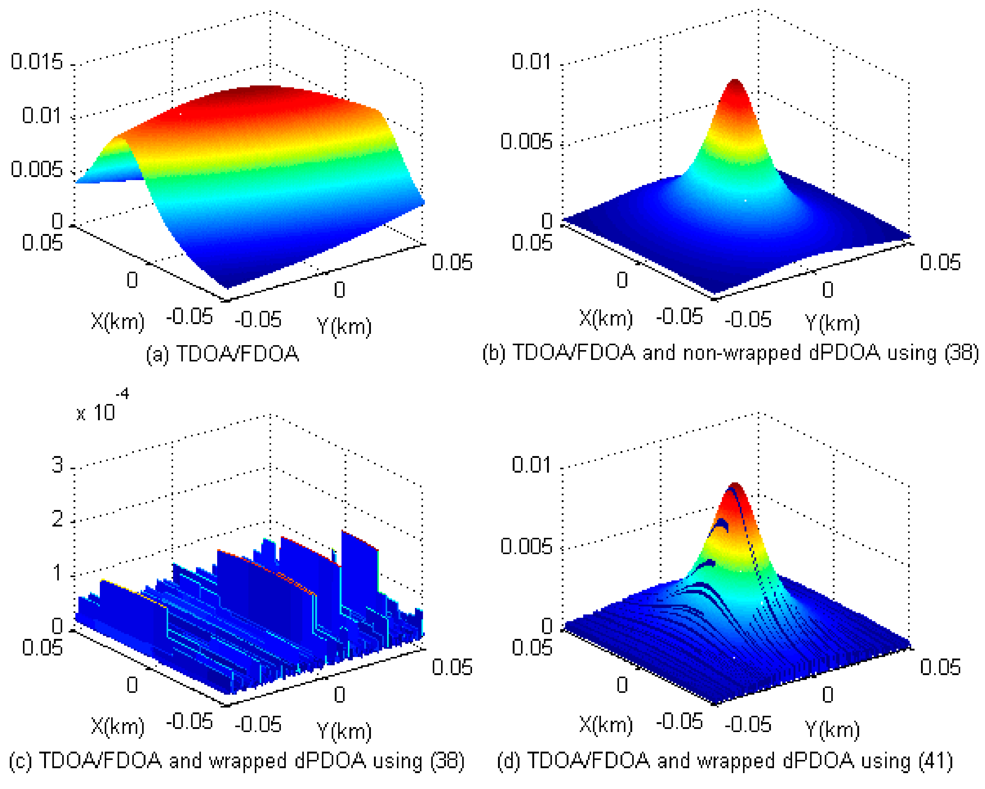
3.1. Solutions for Phase Wrapping Problem

First, the rough estimation of the target position $u_o$ was solved by the two step algorithm [24]. Then, the grid was divided in a small range with its center around the rough estimation of the target position. When the phase wrapping problem is nonexistent, the cost functions for TDOA/FDOA/PDOA and TDOA/FDOA/dPDOA localization scenarios are given, respectively, as follows.

$$\begin{array}{l}Cos{t}_1\left(x,y\right)={\left({\alpha }_1-{\left.{\alpha }_1\right|}_{u=u_o}\right)}^T{Q}_1^{-1}\left({\alpha }_1-{\left.{\alpha }_1\right|}_{u=u_o}\right)\\ ={\left(r-{\left.r\right|}_{u=u_o}\right)}^T{Q}_r^{-1}\left(r-{\left.r\right|}_{u=u_o}\right)+{\left(\dot{r}-{\left.\dot{r}\right|}_{u=u_o}\right)}^T{\dot{Q}}_r^{-1}\left(\dot{r}-{\left.\dot{r}\right|}_{u=u_o}\right)\\ +{\left(\mathsf{\psi }-{\left.\mathsf{\psi }\right|}_{u=u_o}\right)}^T{Q}_{\psi }^{-1}\left(\mathsf{\psi }-{\left.\mathsf{\psi }\right|}_{u=u_o}\right)\end{array}$$

(37)

$$\begin{array}{l}Cos{t}_2\left(x,y\right)={\left({\alpha }_2-{\left.{\alpha }_2\right|}_{u=u_o}\right)}^T{Q}_2^{-1}\left({\alpha }_2-{\left.{\alpha }_2\right|}_{u=u_o}\right)\\ ={\left(r-{\left.r\right|}_{u=u_o}\right)}^T{Q}_r^{-1}\left(r-{\left.r\right|}_{u=u_o}\right)+{\left(\dot{r}-{\left.\dot{r}\right|}_{u=u_o}\right)}^T{\dot{Q}}_r^{-1}\left(\dot{r}-{\left.\dot{r}\right|}_{u=u_o}\right)\\ +{\left(\Phi -{\left.\Phi \right|}_{u=u_o}\right)}^T{Q}_{\mathrm{\Phi }}^{-1}\left(\Phi -{\left.\Phi \right|}_{u=u_o}\right).\end{array}$$

(38)

Due to the existence of the phase wrapping problem, PDOA and dPDOA measurements may contain a period ambiguity of $2\pi$, which is shown in Figure 6b,c; the optimal position of the target cannot be estimated by (37) and (38). Therefore, it is necessary to modify the cost functions.

For the case of precise phase synchronization between observation stations, the measured PDOA and the calculated PDOA $\left(\mathsf{\psi }-{\left.\mathsf{\psi }\right|}_{u=u_o}\right)$ in (37) are prone to cycle reversal error. Thus, the following modifications are utilized.

$$\begin{array}{l}if\hspace{1em}\hspace{1em}\left(\mathrm{mod}\left(\mathsf{\psi }\right)-\mathrm{mod}\left({\left.\mathsf{\psi }\right|}_{u=u_o}\right)\right)\ge \pi \\ \mathrm{\Delta }\mathsf{\psi }=\left(\mathrm{mod}\left(\mathsf{\psi }\right)-\mathrm{mod}\left({\left.\mathsf{\psi }\right|}_{u=u_o}\right)\right)-2\pi \\ elseif\hspace{1em}\left(\mathrm{mod}\left(\mathsf{\psi }\right)-\mathrm{mod}\left({\left.\mathsf{\psi }\right|}_{u=u_o}\right)\right)\le -\pi \\ \mathrm{\Delta }\mathsf{\psi }=\left(\mathrm{mod}\left(\mathsf{\psi }\right)-\mathrm{mod}\left({\left.\mathsf{\psi }\right|}_{u=u_o}\right)\right)-2\pi \\ end\end{array}$$

(39)

where $\mathrm{mod}\left(\right)$ is the function that limits the term between $-\pi$ and $\pi$. In this time, cost function in (37) for TDOA/FDOA/PDOA method can be modified as:

$$\begin{array}{l}Cos{t}_3\left(x,y\right)={\left(r-{\left.r\right|}_{u=u_o}\right)}^T{Q}_r^{-1}\left(r-{\left.r\right|}_{u=u_o}\right)+{\left(\dot{r}-{\left.\dot{r}\right|}_{u=u_o}\right)}^T{\dot{Q}}_r^{-1}\left(\dot{r}-{\left.\dot{r}\right|}_{u=u_o}\right)\\ +{\left({\left.\mathrm{\Delta }\mathsf{\psi }\right|}_{u=u_o}\right)}^T{Q}_{\psi }^{-1}\left({\left.\mathrm{\Delta }\mathsf{\psi }\right|}_{u=u_o}\right).\end{array}$$

(40)

When the phases are asynchronous between observation stations, there are unknown asynchronous phases. Because the measured PDOA still exhibits period ambiguity with $2\pi$, the measured dPDOA and the calculated dPDOA $\left(\Phi -{\left.\Phi \right|}_{u=u_o}\right)$ in (38) are prone to cycle reversal error. Thus, PDOA is corrected based on (39) and substituted into (38), then the corrected cost function is expressed as:

$$\begin{array}{l}Cos{t}_4\left(x,y\right)={\left(r-{\left.r\right|}_{u=u_o}\right)}^T{Q}_r^{-1}\left(r-{\left.r\right|}_{u=u_o}\right)+{\left(\dot{r}-{\left.\dot{r}\right|}_{u=u_o}\right)}^T{\dot{Q}}_r^{-1}\left(\dot{r}-{\left.\dot{r}\right|}_{u=u_o}\right)\\ +{\left(B{\left.\mathrm{\Delta }\mathsf{\psi }\right|}_{u=u_o}\right)}^T{Q}_{\mathrm{\Phi }}^{-1}\left(B{\left.\mathrm{\Delta }\mathsf{\psi }\right|}_{u=u_o}\right)\end{array}$$

(41)

where $B$ is defined in (18).

The phase wrapping problems are solved based on the modified cost functions in (40) and (41) for TDOA/FDOA/PDOA and TDOA/FDOA/dPDOA, respectively.

The estimation of target position can be obtained directly from the modified cost functions for both TDOA/FDOA/PDOA and TDOA/FDOA/dPDOA scenarios. However, the computation overhead is significantly high. Iterative localization algorithms based on maximum likelihood (ML) are proposed in Section 3.2.

3.2. Iterative ML Estimation Algorithms

In this section, two iterative ML estimation algorithms are proposed for TDOA/FDOA/PDOA and TDOA/FDOA/dPDOA methods, respectively. First, the two step localization algorithm in [24] is utilized to estimate a rough position of the target by TDOA and FDOA information. Then, iterative ML estimation algorithms are proposed for TDOA/FDOA/PDOA and TDOA/FDOA/dPDOA methods, respectively.

3.2.1. ML Estimator for Precise Phase Synchronization

For the case of the no phase wrapping problem, the measurement vector is ${\alpha }_1={\left[r^T,{\dot{r}}^T,{\mathsf{\psi }}^T\right]}^T$, and the measurement equation can be expressed as:

$$\mathrm{\Delta }{\alpha }_1={\alpha }_1-{\alpha }_1^o={\alpha }_1-\left({\alpha }_1{|}_{u=u_o}\right)-\left(\frac{\partial {\alpha }_1}{\partial u}{|}_{u=u_o}\right)\left(u-u_o\right).$$

(42)

According to the weighted least squares method, the iterative step $\delta \widehat{\mathit{u}}$ can be estimated as:

$$\delta \widehat{\mathit{u}}={\left[{\left(\frac{\partial {\alpha }_1}{\partial \mathit{u}}{|}_{\mathit{u}={\mathit{u}}_o}\right)}^T{\mathit{Q}}_1^{-1}\left(\frac{\partial {\alpha }_1}{\partial \mathit{u}}{|}_{\mathit{u}={\mathit{u}}_o}\right)\right]}^{-1}{\left(\frac{\partial {\alpha }_1}{\partial \mathit{u}}{|}_{\mathit{u}={\mathit{u}}_o}\right)}^T{\mathit{Q}}_1^{-1}\left[{\alpha }_1-\left({\alpha }_1{|}_{\mathit{u}={\mathit{u}}_o}\right)\right]$$

(43)

where:

$$\frac{\partial {\alpha }_1}{\partial \mathit{u}}{|}_{\mathit{u}={\mathit{u}}_o}={\left[\begin{array}{ccc}{\left(\frac{\partial r}{\partial \mathit{u}}\right)}^T& {\left(\frac{\partial \dot{r}}{\partial \mathit{u}}\right)}^T& {\left(\frac{\partial \psi }{\partial \mathit{u}}\right)}^T\end{array}\right]}^T{|}_{\mathit{u}={\mathit{u}}_o}$$

(44)

$${\mathit{Q}}_1=\left[\begin{array}{ccc}{\mathit{Q}}_r& & \\ & {\dot{\mathit{Q}}}_r& \\ & & {\mathit{Q}}_{\psi }\end{array}\right].$$

(45)

Then, the formula for the first iteration is:

$$u^{(1)}=u_o+\delta \widehat{u}.$$

(46)

Iterative optimization is completed until $‖\delta \widehat{u}‖$ is less than the threshold.

In addition, if there is a phase wrapping problem in the actual PDOA measurements, (43) is corrected based on the modified cost function in (40).

$$\delta \widehat{\mathit{u}}={\left[{\left(\frac{\partial {\alpha }_1}{\partial \mathit{u}}{|}_{\mathit{u}={\mathit{u}}_o}\right)}^T{\mathit{Q}}_1^{-1}\left(\frac{\partial {\alpha }_1}{\partial \mathit{u}}{|}_{\mathit{u}={\mathit{u}}_o}\right)\right]}^{-1}{\left(\frac{\partial {\alpha }_1}{\partial \mathit{u}}{|}_{\mathit{u}={\mathit{u}}_o}\right)}^T{\mathit{Q}}_1^{-1}\left[\begin{array}{c}\mathit{r}-{\left.\mathit{r}\right|}_{\mathit{u}={\mathit{u}}_o}\\ \dot{\mathit{r}}-{\left.\dot{\mathit{r}}\right|}_{\mathit{u}={\mathit{u}}_o}\\ {\left.\mathrm{\Delta }\psi \right|}_{\mathit{u}={\mathit{u}}_o}\end{array}\right]$$

(47)

where ${\left.\mathrm{\Delta }\psi \right|}_{\mathit{u}={\mathit{u}}_o}$ is defined in (39).

3.2.2. ML Estimator for Phase Asynchronization

If there is no phase wrapping problem, the measurement vector is ${\alpha }_2={\left[r^T,{\dot{r}}^T,{\Phi }^T\right]}^T$, and the iterative step $\delta \widehat{\mathit{u}}$ can be estimated as:

$$\delta \widehat{\mathit{u}}={\left[{\left(\frac{\partial {\alpha }_2}{\partial \mathit{u}}{|}_{\mathit{u}={\mathit{u}}_o}\right)}^T{\mathit{Q}}_2^{-1}\left(\frac{\partial {\alpha }_2}{\partial \mathit{u}}{|}_{\mathit{u}={\mathit{u}}_o}\right)\right]}^{-1}{\left(\frac{\partial {\alpha }_2}{\partial \mathit{u}}{|}_{\mathit{u}={\mathit{u}}_o}\right)}^T{\mathit{Q}}_2^{-1}\left[{\alpha }_2-\left({\alpha }_2{|}_{\mathit{u}={\mathit{u}}_o}\right)\right]$$

(48)

where:

$$\frac{\partial {\alpha }_2}{\partial \mathit{u}}{|}_{\mathit{u}={\mathit{u}}_o}={\left[\begin{array}{ccc}{\left(\frac{\partial r}{\partial \mathit{u}}\right)}^T& {\left(\frac{\partial \dot{r}}{\partial \mathit{u}}\right)}^T& {\left(\frac{\partial \mathit{\Phi }}{\partial \mathit{u}}\right)}^T\end{array}\right]}^T{|}_{\mathit{u}={\mathit{u}}_o}$$

(49)

$${\mathit{Q}}_2=\left[\begin{array}{ccc}{\mathit{Q}}_r& & \\ & {\dot{\mathit{Q}}}_r& \\ & & {\mathit{Q}}_{\Phi }\end{array}\right].$$

(50)

Then, the formula for the first iteration is:

$$u^{(1)}=u_o+\delta \widehat{u}.$$

(51)

Iterative optimization is completed until $‖\delta \widehat{u}‖$ is less than the threshold.

In addition, if there is a phase wrapping problem in the actual PDOA measurement, (48) is corrected based on the modified cost function in (41).

$$\delta \widehat{\mathit{u}}={\left[{\left(\frac{\partial {\alpha }_2}{\partial \mathit{u}}{|}_{\mathit{u}={\mathit{u}}_o}\right)}^T{\mathit{Q}}_2^{-1}\left(\frac{\partial {\alpha }_2}{\partial \mathit{u}}{|}_{\mathit{u}={\mathit{u}}_o}\right)\right]}^{-1}{\left(\frac{\partial {\alpha }_2}{\partial \mathit{u}}{|}_{\mathit{u}={\mathit{u}}_o}\right)}^T{\mathit{Q}}_2^{-1}\left[\begin{array}{c}\mathit{r}-{\left.\mathit{r}\right|}_{\mathit{u}={\mathit{u}}_o}\\ \dot{\mathit{r}}-{\left.\dot{\mathit{r}}\right|}_{\mathit{u}={\mathit{u}}_o}\\ {\left.\mathit{B}\mathrm{\Delta }\psi \right|}_{\mathit{u}={\mathit{u}}_o}\end{array}\right]$$

(52)

where ${\left.\mathrm{\Delta }\psi \right|}_{\mathit{u}={\mathit{u}}_o}$ is defined in (39).

4. Simulations

In this section, the authors first analyze the geographic distribution figures of different cost functions for the phase wrapping solution. Then, the performances of the proposed ML estimation algorithms are compared with their CRLBs respectively.

4.1. Simulations for Phase Wrapping Solution

The simulation scenarios are the same as those in Section 2.2.3, which is utilized in [36]. The simulations with precise phase synchronization between observation stations are shown in Figure 7. Figure 7a shows the distribution of cost function using only TDOA and FDOA information. Figure 7b shows the distribution of cost function in (37) with non-wrapped PDOA. Figure 7c shows the distribution of cost function in (37) with wrapped PDOA. Figure 7d shows the distribution of modified cost function in (40) with wrapped PDOA.

As can be seen from the comparison of the cost function in Figure 7a,b, due to the increase in PDOA information, the cost function peak in Figure 7b is sharper than that in Figure 7a, which corresponds to higher localization accuracy. However, as shown in Figure 7b,c, the simulation in Figure 7c cannot estimate the target position while the simulation corresponding to Figure 7b can accurately estimate the target position. This is because the cost function in (37) is relatively ideal and can only be applied to the situation with phase non-ambiguity. By comparing Figure 7b,d, it can be seen that the cost function distribution figures are almost the same. The simulation corresponding to Figure 7d could estimate the target position accurately, which proves the modified cost function in (40) can be used for wrapped PDOA.

Figure 8 gives the simulations for the scenario of phase asynchronization between observation stations. Figure 8a shows the distribution of cost function using only TDOA and FDOA information. Figure 8b shows the distribution of cost function in (38) with the use of non-wrapped dPDOA information. Figure 8c shows the distribution of cost function in (38) with the use of wrapped dPDOA information directly. Figure 8d shows the distribution of modified cost function in (41) with the use of wrapped dPDOA information.

As can be seen from the comparison of the cost functions in Figure 8a,b, due to the increase in dPDOA information, the cost function peak in Figure 8b is sharper than that in Figure 8a, which means higher localization accuracy. However, comparing Figure 7b and Figure 8b, the cost function peak is sharper in Figure 7b, so PDOA information can improve localization accuracy more effectively, which is consistent with the simulations of the CRLB analysis in Section III. As shown in Figure 8b,c, the simulation corresponding to Figure 8c cannot estimate the target position, while the simulation corresponding to Figure 8b can estimate the target position accurately. This is because the cost function in (38) is relatively ideal and can only be applied for the situation with phase non-ambiguity and cannot be realized in most practical applications. By comparing Figure 8b,d, it can be seen that the figures of cost function distribution are almost the same. The simulation corresponding to Figure 8d can accurately estimate the target position, which proves the modified cost function in (41) can be used for the case of wrapped dPDOA.

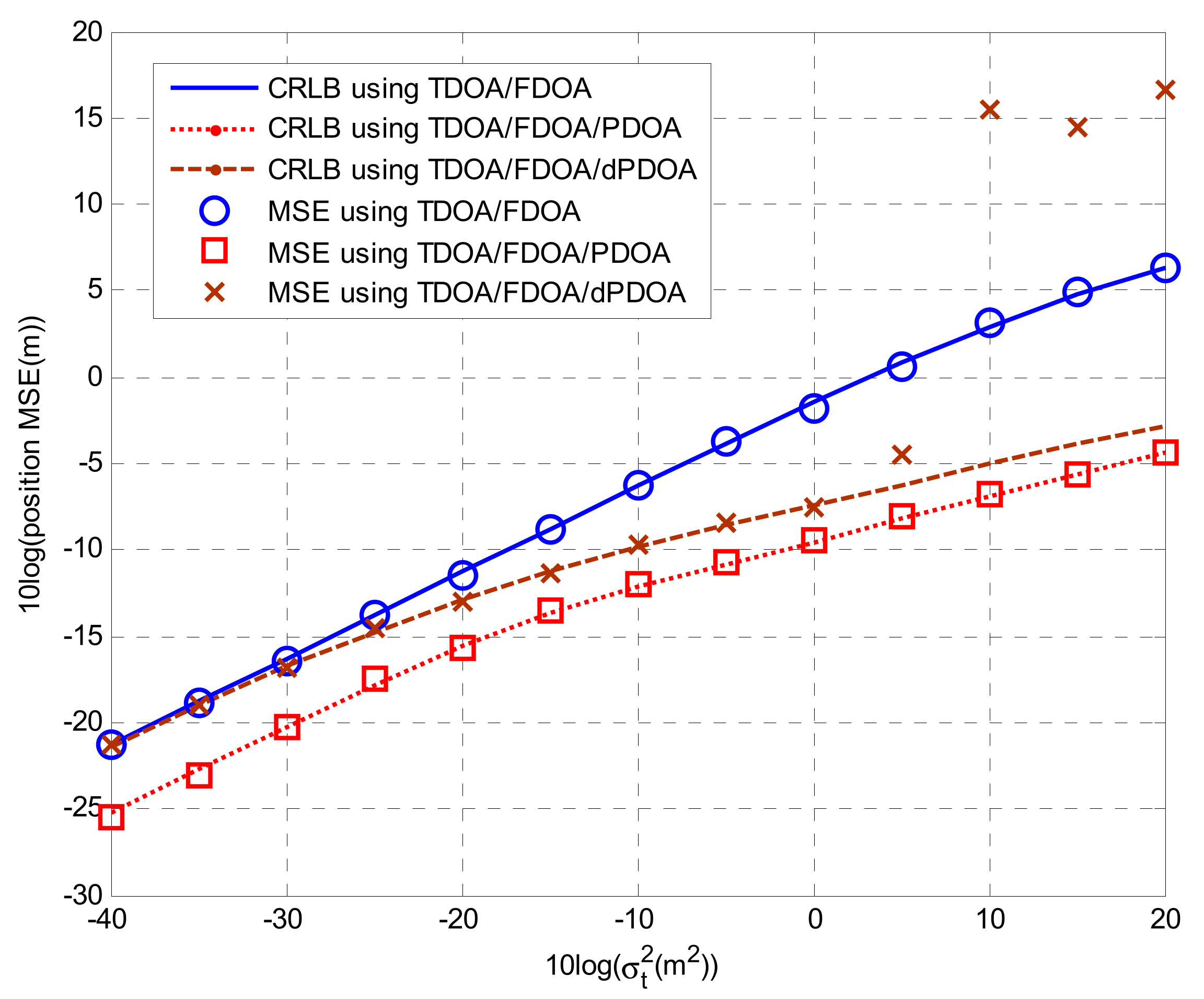
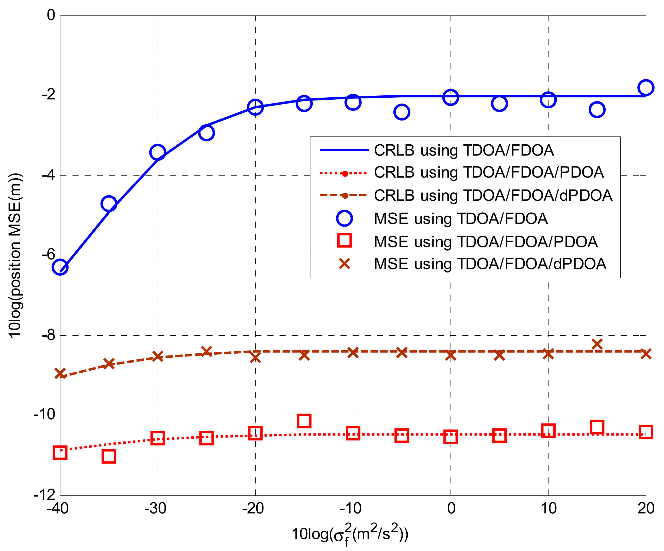
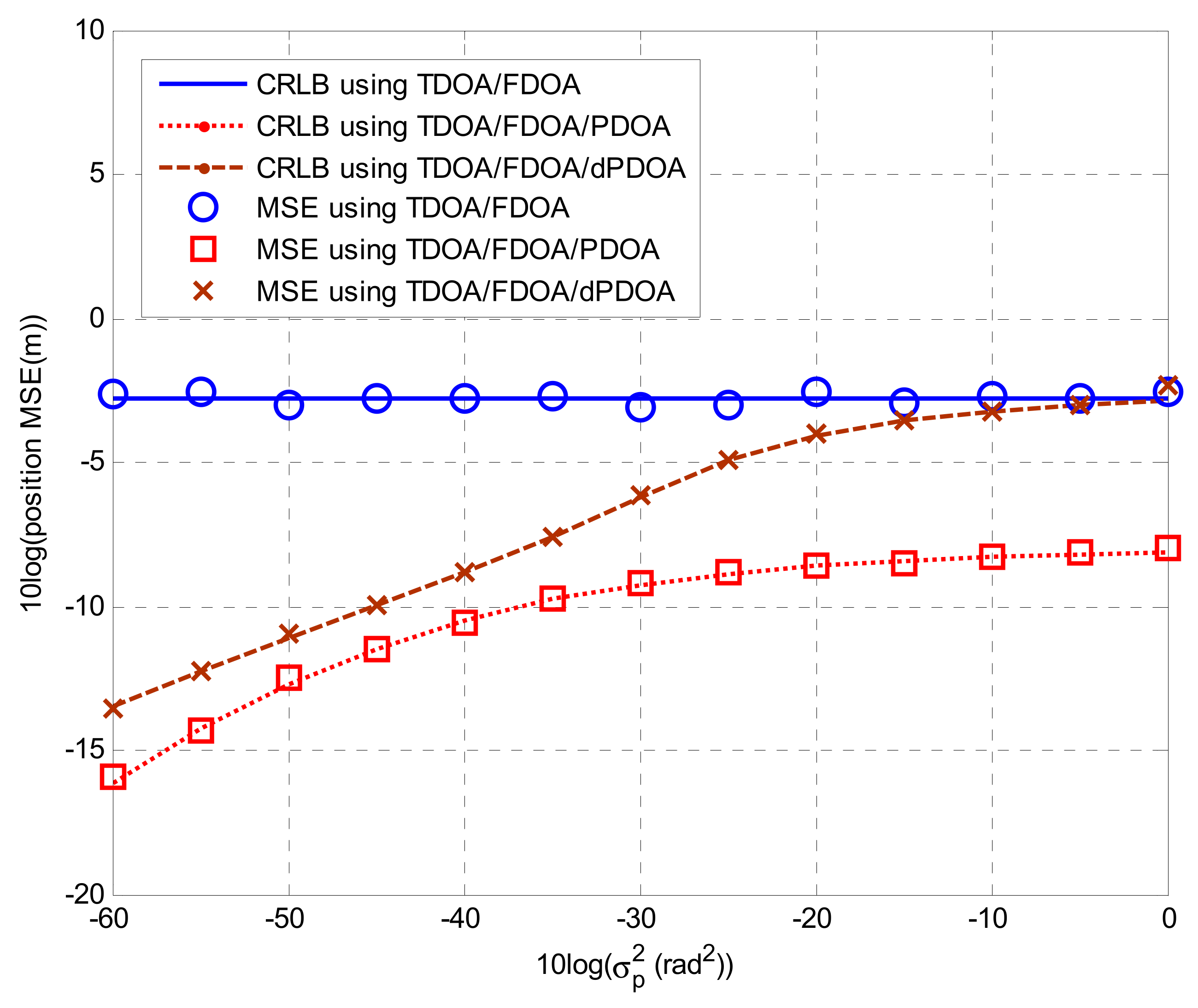
4.2. Solutions for Localization Algorithms

The simulation scenarios in this section are generated randomly. The positions of four stations are generated randomly among the area of (−10,000, −10,000), (−10,000, 10,000), (10,000, 10,000) and (10,000, −10,000). The velocities of four stations are generated randomly between (−100, −100) and (100, 100). The number of random scenarios is 100. For every random scenario, the measurements of TDOA, FDOA and PDOA are generated with 100 Monte Carlo runs. The CRLBs and MSEs in Figure 9,Figure 10,Figure 11 and Figure 12 are generated by the average of the 100 random scenarios.

In a real scenario, the motions of receiving stations, such as satellites and airplanes, is very complicated. In this manuscript, we want to focus on the theoretical performance and ML estimation algorithms of TDOA/FDOA/PDOA and TDOA/FDOA/dPDOA localization scenarios. The simulation scenario is not a real case, and the measurements of TDOA, FDOA and PDOA are generated by theoretical value and Gaussian white noise.

At first, ${\sigma }_f^2$, ${\sigma }_p^2$ and $K$ are fixed at 0.1, ${10}^{-4}$ and 10. The localization performances of different localization systems are analyzed with different TDOA measurement errors. As shown in Figure 9, the TDOA/FDOA localization method and TDOA/FDOA/PDOA localization method can fully reach their respective CRLBs. The TDOA/FDOA/dPDOA localization method will deviate from CRLB when TDOA measurement error ${\sigma }_t^2$ is larger than 5 dB.

Then, ${\sigma }_t^2$, ${\sigma }_p^2$ and $K$ are fixed at 1, ${10}^{-4}$ and 10. The localization performances of different localization systems are analyzed with different FDOA measurement errors. According to Figure 10, three localization methods can approximately reach their respective CRLBs with different FDOA measurement errors for this scenario.

Furthermore, ${\sigma }_t^2$, ${\sigma }_f^2$ and $K$ are fixed at 1, 0.1 and 10. The localization performances of different localization systems are analyzed with different PDOA measurement errors. As shown in Figure 11, three localization methods can approximately reach their respective CRLBs with different PDOA measurement errors in the simulation. It is worth noting that when PDOA measurement error is large, adding dPDOA information hardly improves the localization accuracy, which is coincident with the CRLB analysis in Section 2.2.3.

Finally, ${\sigma }_t^2$, ${\sigma }_f^2$ and ${\sigma }_p^2$ are fixed at 1, 0.1 and ${10}^{-4}$. The localization performance of different localization systems are analyzed with different $K$. It can be seen from Figure 12 that with the increase in the number of signal segments, the localization error decreases gradually, and all the localization algorithms can approximately reach their respective CRLBs.

5. Conclusions

This paper studied the methods of using PDOA information to improve position accuracy of joint TDOA and FDOA localization scenarios. For the cases of phase synchronization and asynchronization between observation stations, the authors first derived the CRLBs of TDOA/FDOA/PDOA and TDOA/FDOA/dPDOA localization methods. The CRLB comparisons showed the added information of PDOA could improve the localization performance obviously for different situations. Due to the phase wrapping in PDOA or dPDOA information, the influence on localization performance was analyzed. Then, solutions for phase wrapping problem were proposed for the localization scenarios of TDOA/FDOA/PDOA and TDOA/FDOA/dPDOA. Finally, two iterative ML estimation algorithms were presented for TDOA/FDOA/PDOA and TDOA/FDOA/dPDOA methods, respectively. Simulation results showed the proposed solutions for the phase wrapping problem are effective, and the ML estimators could achieve their CLRBs. In addition, due to no requirement for phase precision synchronization between observation stations, if the phases of receivers are stable and unchanging, the TDOA/FDOA/dPDOA localization method is more suitable for outdoor scenarios, while the TDOA/FDOA/PDOA localization method may be more suitable for indoor scenarios, where phase synchronization is more easy to accomplish. In future work, we will validate the proposed algorithms by outfield experiments.

References

1. Cater, G.C. Time Delay Estimation for Passive Sonar Signal Processing. IEEE Trans. Acoust. Speech Signal Process. 1981, 29, 462–470. [Google Scholar]
2. Weinstein, E. Optimal Source Localization and Tracking from Passive Array Measurements. IEEE Trans. Acoust. Speech Signal Process. 1982, 30, 69–76. [Google Scholar] [CrossRef]
3. Murata, M.; Ahmetovic, D.; Sato, D.; Takagi, H.; Kitani, K.M.; Asakawa, C. Smartphone-based Indoor Localization for Blind Navigation Across Building Complexes. In Proceedings of the 2018 IEEE International Conference on Pervasive Computing and Communications (PerCom), Athens, Greece, 19–23 March 2018; pp. 1–10. [Google Scholar]
4. Fan, L.; Zhou, C. 3D Lightning Location Method Based on Range Difference Space Projection. Remote Sens. 2022, 14, 1003. [Google Scholar] [CrossRef]
5. Yang, G.; Shi, X.; Feng, L.; He, S.; Shi, Z.; Chen, J. CEDAR: A Cost-effective Crowdsensing System for Detecting and Localizing Drones. IEEE Trans. Mobile Comput. 2019, 19, 2028–2043. [Google Scholar] [CrossRef]
6. Wang, Y.; Zhou, T.; Yi, W.; Kong, L. A GDOP-Based Performance Description of TOA Localization with Uncertain Measurements. Remote Sens. 2022, 14, 910. [Google Scholar] [CrossRef]
7. Sun, Y.; Ho, K.C.; Wan, Q. Solution and Analysis of TDOA Localization of a Near or Distant Source in Close Form. IEEE Trans. Signal Process. 2019, 67, 320–335. [Google Scholar] [CrossRef]
8. Wang, Y.; Sun, G.-C.; Wang, Y.; Yang, J.; Zhang, Z.; Xing, M. A Multi-Pulse Cross Ambiguity Function for the Wideband TDOA and FDOA to Locate an Emitter Passively. Remote Sens. 2022, 14, 3545. [Google Scholar] [CrossRef]
9. Wei, H.-W.; Peng, R.; Wan, Q.; Chen, Z.-X.; Ye, S.-F. Multidimensional Scaling Analysis for Passive Moving Target Localization with TDOA and FDOA Measurements. IEEE Trans. Signal Process. 2010, 58, 1677–1688. [Google Scholar]
10. Sun, Y.; Ho, K.C.; Wan, Q. Eigenspace Solution for AOA Localization in Modified Polar Representation. IEEE Trans. Signal Process. 2020, 68, 2256–2271. [Google Scholar] [CrossRef]
11. Vidal-Valladares, M.G.; Díaz, M.A. A Femto-Satellite Localization Method Based on TDOA and AOA Using Two CubeSats. Remote Sens. 2022, 14, 1101. [Google Scholar] [CrossRef]
12. Jiang, X.; Li, N.; Guo, Y.; Yu, D.; Yang, S. Localization of Multiple RF Sources Based on Bayesian Compressive Sensing Using a Limited Number of UAVs With Airborne RSS Sensor. IEEE Sens. J. 2021, 21, 7067–7079. [Google Scholar] [CrossRef]
13. Huang, S.; Wang, B.; Zhao, Y.; Luan, M. Near-field RSS-based Localization Algorithms Using Reconfigurable Intelligent Surface. IEEE Sens. J. 2022, 22, 3493–3505. [Google Scholar] [CrossRef]
14. Foy, W.H. Position-localization Solutions by Taylor-series Estimation. IEEE Trans. Aerosp. Electron. Syst. 1976, 12, 187–194. [Google Scholar]
15. Chan, Y.T.; Ho, K.C. A Simple and Efficient Estimator for Hyperbolic Localization. IEEE Trans. Signal Process. 1994, 42, 1905–1915. [Google Scholar] [CrossRef]
16. Mikhalev, A.; Ormondroyd, R.F. Comparison of Hough Transform and Particle Filter Methods of Emitter Geolocalization Using Fusion of TDOA Data. In Proceedings of the 2007 4th Workshop Positioning, Navigation and Communication, Hannover, Germany, 22 March 2007; pp. 121–127. [Google Scholar]
17. Bin, Y.Z.; Yan, Q.; Nan, L.A. PSO Based Passive Satellite Localization Using TDOA and FDOA Measurements. In Proceedings of the 2011 10th IEEE/ACIS International Conference on Computer and Information Science, Sanya, China, 16–18 May 2011; pp. 251–254. [Google Scholar]
18. Wang, G.; Li, Y.; Ansari, N.A. Semidefinite Relaxation Method for Source Localization Using TDOA and FDOA Measurements. IEEE Trans. Veh. Technol. 2013, 62, 853–862. [Google Scholar] [CrossRef]
19. Weiss, A.J. Direct Position Determination of Narrowband Radio Frequency Transmitters. IEEE Signal Process. Lett. 2004, 11, 513–516. [Google Scholar] [CrossRef]
20. Weiss, A.J. Direct Geolocalization of Wideband Emitters Based on Delay and Doppler. IEEE Trans. Signal Process. 2011, 59, 2513–2521. [Google Scholar] [CrossRef]
21. Li, J.; Yang, L.; Guo, F.; Jiang, W. Coherent Summation of Multiple Short-time Signals for DirectPositioning of a Wideband Source Based on Delay and Doppler. Digit. Signal Process. 2016, 48, 58–70. [Google Scholar] [CrossRef]
22. Ma, F.; Liu, Z.-M.; Guo, F. Direct Position Determination for Wideband Sources Using Fast Approximation. IEEE Trans. Veh. Technol. 2019, 68, 8216–8221. [Google Scholar] [CrossRef]
23. Ma, F.; Guo, F.; Yang, L. Direct Position Determination of Moving Sources Based on Delay and Doppler. IEEE Sens. J. 2020, 20, 7859–7869. [Google Scholar]
24. Ho, K.C.; Lu, X.; Kovavisaruch, L. Source Localization Using TDOA and FDOA Measurements in the Presence of Receiver Localization Errors: Analysis and Solution. IEEE Trans. Signal Process. 2007, 55, 684–696. [Google Scholar] [CrossRef]
25. Hmam, H. Optimal Sensor Velocity Configuration for TDOA-FDOA Geolocalization. IEEE Trans. Signal Process. 2017, 65, 628–637. [Google Scholar] [CrossRef]
26. Elgamoudi, A.; Benzerrouk, H.; Elango, G.A.; Landry, R. Gauss Hermite H Filter for UAV Tracking Using LEO Satellites TDOA/FDOA Measurement—Part I. IEEE Access 2020, 8, 201428–201440. [Google Scholar] [CrossRef]
27. Wolf, F.; Berg, V.; Dehmas, F.; Mannoni, V.; de Rivaz, S. Multi-Frequency Phase Difference of Arrival for Precise Localization in Narrowband LPWA Networks. In Proceedings of the ICC 2021—IEEE International Conference on Communications, Montreal, QC, Canada, 14–23 June 2021; pp. 1–6. [Google Scholar]
28. Zhang, K.; Shen, C.; Bao, M.; Vaniushkina, D.; Kumushai, K.; Zang, L. Research on Optimization Algorithm Based on PDOA. In Proceedings of the 2021 IEEE 21st International Conference on Communication Technology (ICCT), Tianjin, China, 13–16 October 2021; pp. 1427–1430. [Google Scholar]
29. Sippel, E.; Hehn, M.; Koegel, T.; Groschel, P.; Hofmann, A.; Bruckner, S.; Geiss, J.; Schober, R.; Vossiek, M. Quasi-Coherent Phase-Based Localization and Tracking of Incoherently Transmitting Radio Beacons. IEEE Access 2021, 9, 133229–133239. [Google Scholar] [CrossRef]
30. Gashi, M.; Botler, L.; Koutroulis, G.; Diwold, K. Poster Abstract: Accurate and Efficient Hybrid Indoor Localization using ML Methods. In Proceedings of the 2022 21st ACM/IEEE International Conference on Information Processing in Sensor Networks (IPSN), Milano, Italy, 4–6 May 2022; pp. 523–524. [Google Scholar]
31. Ma, Y.; Wang, B.; Pei, S.; Zhang, Y.; Zhang, S.; Yu, J. An Indoor Localization Method Based on AOA and PDOA Using Virtual Stations in Multipath and NLOS Environments for Passive UHF RFID. IEEE Access 2018, 6, 31772–31782. [Google Scholar] [CrossRef]
32. Zhang, S.; Du, P.; Chen, C.; Zhong, W.-D.; Alphones, A. Robust 3D Indoor VLP System Based on ANN Using Hybrid RSS/PDOA. IEEE Access 2019, 7, 47769–47780. [Google Scholar] [CrossRef]
33. Peng, C.; Jiang, H.; Qu, L. Deep Convolutional Neural Network for Passive RFID Tag Localization Via Joint RSSI and PDOA Fingerprint Features. IEEE Access 2021, 9, 15441–15451. [Google Scholar] [CrossRef]
34. Chen, H.; Ballal, T.; Saeed, N.; Alouini, M.-S.; Ai-Naffouri, T.Y. A joint TDOA-PDOA localization approach using particle swarm optimization. IEEE Wirel. Commun. Lett. 2020, 9, 1240–1244. [Google Scholar] [CrossRef]
35. Zhang, S.; Zhong, W.-D.; Du, P.; Chen, C. Experimental Demonstration of Indoor Sub-Decimeter Accuracy VLP System Using Differential PDOA. IEEE Photonics Technol. Lett. 2018, 30, 1703–1706. [Google Scholar] [CrossRef]
36. Yeredor, A.; Angel, E. Joint TDOA and FDOA Estimation: A Conditional Bound and Its Use for Optimally Weighted Localization. IEEE Trans. Signal Process. 2011, 59, 1612–1623. [Google Scholar] [CrossRef]
Figure 1. The localization geometry.
Remotesensing 15 00915 g001
Figure 2. CRLBs comparison with the variation in TDOA noise σ t 2 .
Remotesensing 15 00915 g002
Figure 3. CRLBs comparison with the variation in FDOA noise σ f 2 .
Remotesensing 15 00915 g003
Figure 4. CRLBs comparison with the variation in PDOA noise σ p 2 .
Remotesensing 15 00915 g004
Figure 5. CRLBs comparison with the variation in signal segment number K .
Remotesensing 15 00915 g005
Figure 6. Phase wrapping phenomenon of PDOA and dPDOA.
Remotesensing 15 00915 g006
Figure 7. Cost functions comparison for the scenario of phase synchronization.
Remotesensing 15 00915 g007
Figure 8. Cost functions comparison for the scenario of phase asynchronization.
Remotesensing 15 00915 g008
Figure 9. Localization accuracy comparison with the variation in TDOA noise σ t 2 .
Remotesensing 15 00915 g009
Figure 10. Localization accuracy comparison with the variation in FDOA noise σ f 2 .
Remotesensing 15 00915 g010
Figure 11. Localization accuracy comparison with the variation in PDOA noise σ p 2 .
Remotesensing 15 00915 g011
Figure 12. Localization accuracy comparison with the variation in signal segment number K .
Remotesensing 15 00915 g012