Estimating Afforestation Area Using Landsat Time Series and Photointerpreted Datasets

Abstract

Afforestation processes, natural and anthropogenic, involve the conversion of other land uses to forest, and they represent one of the most important land use transformations, influencing numerous ecosystem services. Although remotely sensed data are commonly used to monitor forest disturbance, only a few reported studies have used these data to monitor afforestation. The objectives of this study were two fold: (1) to develop and illustrate a method that exploits the 1985–2019 Landsat time series for predicting afforestation areas at 30 m resolution at the national scale, and (2) to estimate afforestation areas statistically rigorously within Italian administrative regions and land elevation classes. We used a Landsat best-available-pixel time series (1985–2019) to calculate a set of temporal predictors that, together with the random forests prediction technique, facilitated construction of a map of afforested areas in Italy. Then, the map was used to guide selection of an estimation sample dataset which, after a complex photointerpretation phase, was used to estimate afforestation areas and associated confidence intervals. The classification approach achieved an accuracy of 87%. At the national level, the afforestation area between 1985 and 2019 covered 2.8 ± 0.2 million ha, corresponding to a potential C-sequestration of 200 million t. The administrative region with the largest afforested area was Sardinia, with 260,670 ± 58,522 ha, while the smallest area of 28,644 ± 12,114 ha was in Valle d’Aosta. Considering elevation classes of 200 m, the greatest afforestation area was between 400 and 600 m above sea level, where it was 549,497 ± 84,979 ha. Our results help to understand the afforestation process in Italy between 1985 and 2019 in relation to geographical location and altitude, and they could be the basis of further studies on the species composition of afforestation areas and land management conditions.

1. Introduction

1.1. Importance of Afforestation Monitoring

Forests are defined by the Food and Agriculture Organization (FAO) agency of the United Nations as “territory with arboreal coverage greater than 10% compared to an extension greater than 0.5 ha, where the trees reach a minimum height of 5 m when mature and a minimum width of 20 m” [1]. Changes between forest and other land use classes include the gain and the loss of arboreal cover. Afforestation constitutes the gain of arboreal cover and is characterized by the conversion of other land uses to forest, while deforestation constitutes the loss of arboreal cover and is characterized as the conversion of forest to other land uses [2]. According to the FAO definition, afforestation can be natural via spontaneous colonization of vegetation or anthropogenic through trees planting or direct sowing on land that was not previously forested.

Afforestation, one of the most important land use transformations, produces many positive effects. Afforestation processes increase the terrestrial carbon sink, create new ecological corridors, protect soil [3] and water, contribute to combating global warming, and increase biodiversity [4,5]. On the one hand, monitoring afforestation is important for evaluating these positive effects; on the other hand, proper monitoring is also needed to assess the negative impacts that mismanaged afforestation processes may impose on a territory such as loss of grazing habitats [4,5,6,7]. Afforestation may also be a symptom of the effect of climate change, such as in the case of movement of the tree line, the elevation or latitude above which trees give way to shrubs, to higher elevations or latitudes [8]. Finally, because of its important contribution to land use evolution, afforestation processes have a central role in the formulation of policies that aim to preserve forest resources and provide ecosystem services [2].

The agreements stipulated by COP 26 (https://ukcop26.org/it/iniziale/, accessed on 10 May 2022), the actions contained in the EU Forest Strategy [9], the Italian national legislation on forestry and forestry supply chain (legislative decree 34/2018), and the Italian National Forest Strategy [10] all raise the profile and priority of reforestation interventions and the construction of a series of cartographic products that collect information on forest heritage, including afforestation. Afforestation should be considered in reforestation programs, making the analysis of afforestation areas a central feature of forest and landscape planning and management. Because few existing datasets or products with appropriate spatial resolution can be used to monitor afforestation effectively, greater research attention should be focused on the development of accurate and up-to-date tools to support afforestation-related decision-making processes.

1.2. Remote Sensing Support for Afforestation Monitoring: The State of the Art

Remotely sensed data are well suited for land monitoring applications at both global and local scales, facilitating analysis of numerous elements at fine spatial resolution [11] preferably using open access data [12,13], cloud computing platforms, and Big Data processing [14].

Afforestation can be analyzed using remotely sensed data. An afforestation classification model can be constructed using a single model that analyzes observations of change between two dates in both the land cover response variable and changes in remotely sensed predictor variables [15]. This method links trends in afforestation during the observation period to trends in variables or indices such as the Normalized Difference Vegetation Index (NDVI) via a predictive model which is then used to classify the afforestation spectral response [16,17,18].

A currently popular algorithm for automated classification of remotely sensed images is the random forest (RF) algorithm [19], which is a classification algorithm that uses a series of decision trees based on a sample of data. RF can be used with large datasets because it is not severely adversely affected by overfitting [20].

Although forest disturbance monitoring through automated analysis of remotely sensed imagery is a common topic [21,22,23,24,25], afforestation assessment is rarely investigated, being treated as a central subject in only a few studies. Among the studies that consider afforestation prediction, Qiu et al. [26] used MODIS images (500 m spatial resolution) to map afforestation areas between 2001 and 2016, in China. They proposed the automated method for detecting multiple vegetation changes (AMCC) based on five temporal indices. Yin et al. [27] used RF with MODIS data and a modified version of LandTrendr with Landsat images to monitor the effect of re-vegetation programs between 2000 and 2014, in China, while Ramírez-Cuesta et al. [28] used MODIS-based NDVI seasonal variables to analyze the main land cover changes that occurred in Europe between 2000 and 2018, focusing on the maximum value of the NDVI that accurately predicted locations where main changes such as afforestation occurred.

Although these studies achieve large accuracies, products with a spatial resolution of 500 m are not useful for monitoring afforestation in the fragmented and morphologically diverse areas typical of Italy and many other Mediterranean countries. Moreover, afforestation processes are characterized by patches of limited size whose accurate prediction requires finer resolution images.

Zhu et al. [29] illustrated a method for land cover classification and continuous land cover change detection, between 1986 and 2010, using Landsat images. Huang et al. [30] used NDVI to analyze land cover dynamics in China, detecting vegetation gain and loss from 1985 to 2015, and then classified the land cover in 2015. However, this approach is not useful for our purposes because continuous change detection is not effective for predicting afforestation which is characterized by longer development times which, therefore, require longer observation periods than other land-cover change approaches. Further, the complex Italian morphology requires a larger number of vegetation indices for accurate classification, not a single index as illustrated in the Huang approach [30]. For example, a larger number of vegetation indices is needed to accommodate shaded areas created by mountains which can adversely affect the classification by limiting the vegetation spectral response.

Therefore, cartographic data derived from satellite images are effective sources of information for predicting locations of phenomena related to land cover and its changes and for facilitating direct calculation of multiple useful indicators [31]. However, the variability of forest changes which differ in type, magnitude, and definition, can contribute to inaccurate map products and therefore, make maps less suitable for direct estimation of the spatial extent of the phenomena under investigation [32]. Integration of maps and sample reference data is a useful and potentially unbiased approach for increasing the precision of estimates of the phenomenon of interest. Moreover, using map classes as strata for stratified sampling and estimation can reduce the required sample size, and thus, can accelerate the data acquisition and analysis procedures [33,34,35].

Multiple issues related to mapping and monitoring afforestation require additional attention. First, afforestation prediction using remotely sensed data is seldom investigated. Second, stratified sampling that is based on selection of a simple random sample from within each stratum [36] supports both accuracy assessment and rigorous and unbiased statistical estimation [33] in support of remote sensing-assisted land cover classification. Third, training data sample sizes needed for calibration of prediction techniques tend to be very large, but increasing the sample size increases acquisition costs and the time needed for analysis. Fourth, stratified random sampling and estimation can increase accuracies with only moderate sample sizes.

1.3. Objectives of the Study

The objectives of this study were two fold: (1) to develop and illustrate a method that exploits the 1985–2019 Landsat time series for predicting afforestation areas at 30 m resolution at the national scale, and (2) to estimate afforestation areas statistically and rigorously within Italian administrative regions and land elevation classes using a unique validation sample. We considered two forms of afforestation, both natural through spontaneous colonization of vegetation succession and anthropogenic through planting or direct sowing. Because afforestation contributes to increasing the carbon sink, we also estimated the potential carbon (t of C) that would be sequestered once the forest has matured, in areas where afforestation occurred between 1985 and 2019.

The research was conducted as follows: the study area was the whole area of Italy (Section 2.1.1). To define forest boundaries, we used a forest mask; to define boundaries of Italian administrative regions we used the corresponding shapefile; to define elevation class boundaries, we used a digital elevation model (DEM) (Section 2.1.2). Because vegetative recovery of forest-disturbed areas has a spectral response which could be similar to afforestation and, thereby, decreases model prediction accuracy, and because forest disturbance does not involve any land use change, we considered disturbed forest areas as forest (Section 2.1.5). Afforestation areas were mapped using RF in combination with Landsat best-available-pixel (BAP) composites (Section 2.1.3). We used photointerpetations of reference polygons (Section 2.1.4) in combination with a corresponding subset of BAP composites as a training dataset to calibrate the RF classification algorithm (Section RF Temporal Predictors), which was then used (Section Random Forests) to construct an afforestation map. Then, we selected an estimation dataset of sample points acquired using stratified random sampling with afforestation-based map classes as strata (Section 2.2.2). This sample dataset was used with the map to estimate the afforestation area at the national level and for both administrative regions and elevation classes (Section 2.2.3). Finally, we estimated the carbon that would potentially be sequestered in the afforestation areas (Section 2.2.4).

While RF and Landsat data have been historically used for land cover classification, in this study, they were combined with a statistically rigorous method to estimate afforestation areas at the national level, at the level of the administrative regions, and at the level of elevation classes, to provide relevant results and, more importantly, missing information that was needed for properly supporting decision makers. In more detail, our study had five main outcomes: (1) the afforestation map (Section 3.1), (2) the accuracy assessment (Section 3.2), (3) the afforestation area estimates obtained from the sample data, (4) the map at the national level map for administrative regions and for elevation classes (Section 3.3 and Appendix A), and (5) the estimate of potential C-sequestration in the afforested areas (Section 3.4 and Appendix E). In the Discussion (Section 4) and Conclusions (Section 5) we present the primary results and suggest future research.

2. Materials and Methods

2.1. Materials

Below, we describe the study area (Section 2.1.1), and then we describe the input data used. First, we introduce three country-wide datasets that were used to stratify the study area with respect to (i) forest/non-forest, (ii) administrative regions, and (iii) different elevation classes (Section 2.1.2). Then, the data used to construct the afforestation map are presented: the Landsat best-available-pixel composites that were used as predictors (Section 2.1.3), the reference dataset that was used to train a RF model (Section 2.1.4), and, finally, a forest disturbance mask was used to identify areas that could not be considered afforestation areas (Section 2.1.5). More details are provided in the following sections.

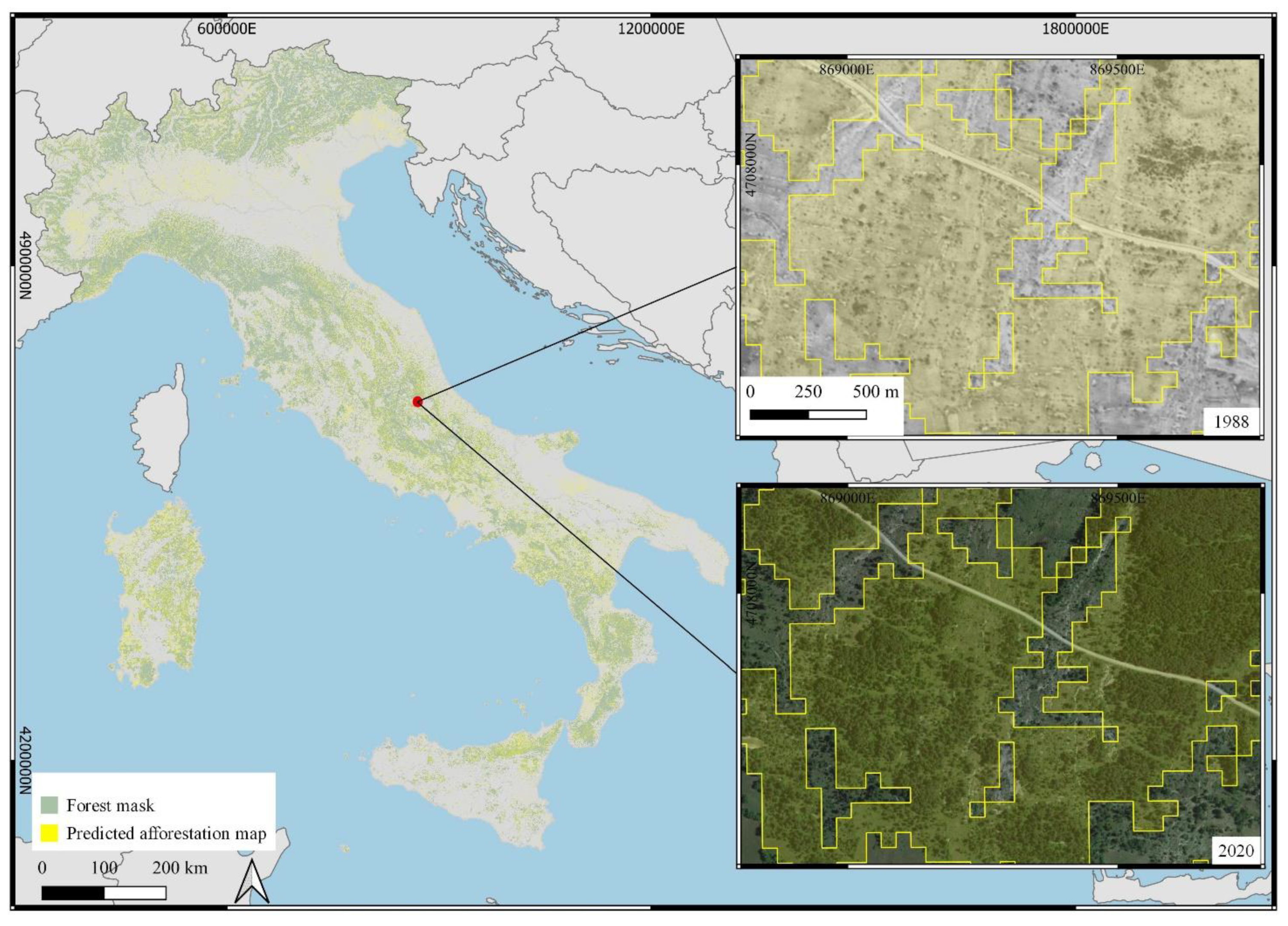
2.1.1. Study Area

The study area included the whole of Italy which covers 301,338 km² and is characterized by mountains (35%), hills (42%), and plains (23%). The maximum elevation of more than 4000 m above sea level (a.s.l.) is observed in the Alps. The climate varies considerably along the Italian peninsula: alpine in the north, continental in internal areas, and Mediterranean along the coasts. Forests occupy almost 35% of the area, about 11 million ha [37]. In some administrative regions, forests cover more than 50% of the territory as in Trentino-Alto Adige, Tuscany, Liguria, Umbria, and Sardinia.

Italian forests are characterized by a rich diversity of plant species, which are predominately deciduous broadleaf forests (Fagus sylvatica, Quercus spp., Castanea sativa, and others), spruce (Picea abies), larch (Larix decidua), black pines (Pinus nigra), and Mediterranean pines forests. Shrublands (above all Mediterranean, thermophilic, and Alpine) cover about one million ha [37].

2.1.2. Forest Mask, Italian Administrative Regions, and Digital Elevation Model

The forest mask of D’Amico et al. [38] was used to distinguish forest from non-forest areas, and therefore, the afforestation process could be analyzed separately inside and outside the forest area as defined by the forest mask. The analysis inside the forest mask, on the one hand, served to identify areas that were previously not forest but are now forest; the analysis outside the mask, on the other hand, served to identify ongoing afforestation, which has not yet been classified by the mask as forest. The mask is based on forest maps for 16 administrative regions at scales between 1:5000 and 1:25,000 and was supplemented with Corine Land Cover or Corine Biotopes data for administrative regions where data were not available. The photointerpretaion was performed using aerial orthophotos, overcoming the limit of the MMU of the input data.. The data were standardized in the reference system, rasterized, and reclassified into “forest” and “non-forest” where FAO defines forest as having canopy cover greater than 10% and minimum area of 0.5 ha [1]. These operations resulted in a 23 × 23 m binary forest/non-forest map with accuracy greater than 85% [39]. Moreover, to predict afforestation areas within administrative regions and elevation classes, the Italian National Institute of Statistics (ISTAT) administrative regions boundary shapefile [40] and the TINITALY/01 DEM with a spatial resolution of 10 m [41,42] were used, respectively.

2.1.3. Landsat Best Available Pixel (BAP) Composite

We used Landsat best-available-pixel (BAP) composites as input data to calibrate the RF classification model and to classify afforestation between 1985 and 2019 by analyzing the trend of 234 temporal predictors (as described in Section RF Temporal Predictors). The BAP composites used as RF calibration data are composed of a subset of the BAP data used to apply the classifier to the study area.

In particular, the BAP data associated with the 1578 training dataset polygons (Section 2.1.4) and the temporal predictors calculated inside training dataset polygons are part of the RF calibration data, while the rest of the BAP composite and the temporal predictors are used as input to the RF classification model applied to the study area.

The BAP procedure was implemented in 2021 in Google Earth Engine (GEE), and the code is openly available (https://code.earthengine.google.com/?accept_repo=users/sfrancini/bap, accessed on 30 January 2022). GEE is a cloud platform for analyzing and processing geospatial data which, by exploiting the computational capacity of Google systems, facilitates the study and monitoring of important environmental phenomena such as changes in land cover including afforestation [14]. GEE makes available and enables the integration of numerous image collections and datasets ready to be processed [43]. GEE permits multiple programming languages, such as Javascript and Python, so that data processing systems can be constructed, easily replicated, and adapted to different situations and needs [44].

GEE provides images preprocessed with respect to multiple factors including surface reflectance and brightness orthorectification (the thermal infrared), atmospheric correction, and cloud masking. We used Landsat 5, 7, and 8 images and all 30 m spatial resolution bands, in the visible spectrum and in the infrared spectrum, to construct the Italian annual composites from 1985 to 2019, from 1 June to 31 August, using the BAP procedure [45]. The period between June and August is usually characterized by the absence of clouds which facilitates acquisition of many clear images. Moreover, the boreal summer is the season in which the photosynthetic activity is greater, thereby producing clearer spectral responses. With BAP, it is possible to obtain a final image that is a composite of the best pixel reflectance values where “best” is characterized using four criteria as defined in White et al., 2014 [46] (i) sensor score to penalize Landsat 7 images where the Scan Line Corrector malfunction (SLC-off) is present; (ii) target day score, to preferably select the images acquired close to a defined acquisition day (in this case 15th of August); (iii) distance to cloud/cloud shadow score, to decrease the scores of those pixels which are in the proximity the cloud cover; and (iv) opacity score (calculated using opacity band produced by LEDAPS), to prefer the pixel with low opacity. Sensor scores and target day are applied to the whole image, while distance to cloud and opacity scores are applied to each pixel.

The BAP application is described on GitHub (https://github.com/saveriofrancini/bap, accessed on 30 January 2022); Griffiths et al., Hermosilla et al. and White et al. [45,46,47,48,49] provide more details.

2.1.4. Training Dataset

The training dataset (Figure 1) was used to define the area to calculate the temporal predictors together with the associated BAP composite to calibrate the RF classification model, which was then applied to the whole of Italy, as described in Section 2.2.1. The training dataset included information for 1578 selected training polygons with sizes ranging from 0.09 ha, the Landsat pixel resolution, to 60 ha, distributed as follows:

• 526 polygons (A) that experienced a change from non-forest to forest between 1985 and 2019;
• 526 polygons (B) in non-forest areas that did not change between 1985 and 2019;
• 526 polygons (C) in forest areas that did not change between 1985 and 2019.

The training dataset was constructed using data from the Land Use Inventory of Italy (IUTI, [50]), which was conducted as part of the Extraordinary Plan of Environmental Remote Sensing by the Italian Ministry of Environment and Protection of Land and Sea in 1990 and was updated between 2000 and 2016. The inventory consists of 1,217,032 randomly selected points that were photointerpreted using a minimum mapping unit (MMU) of 0.5 ha and a minimum mapping width (MMW) of 20 m (RSE < 3%). The classification system considers different land use categories including forest, based on FAO definitions [51]. The 30-year historical dataset can be used to identify areas where afforestation has occurred. We used IUTI data that identify afforestation, and then we added other training data through photointerpretation of composite of BAP (1985–1988), aerial imagery (1988–2012, spatial resolution 50 × 50 cm), and very fine resolution images (2012–2019, spatial resolution 30 × 30 cm).

The training data were selected to represent the diversity of the national Italian forest area and included other cartographic data such as Corine Land Cover, both coniferous and broadleaf forest types and multiple environmental conditions. Photointerpretation of aerial images and very fine resolution images for different years facilitated prediction of areas that had been subject to afforestation and areas that had not been affected by such changes but had maintained either stable forest or stable non-forest cover during the study period. The photointerpretation incorporated the FAO minimum canopy cover percentage of 10% when attributing the forest class (C) to a polygon. A square-meshed grid aligned with the Landsat pixels was constructed so that the photointerpreted polygons corresponded to groups of Landsat pixels. Each polygon was drawn following the shape of the afforestation area and classified as either afforestation, forest, or non-forest classes. The afforestation class was assigned to polygons for which afforestation occurred during the study period and included all areas that satisfied the definition of forest including canopy cover >10% at the end of the afforestation process but excluded areas that did not satisfy the definition such as agricultural areas, mainly olive groves and orchards.

In the afforestation class (A), 44% of the polygons were located at altitudes below 1000 m a.s.l., a percentage that increased to 55% in the forest class (C) and to 72% in the non-forest class (B).

2.1.5. Forest Disturbance Data

Because vegetative recovery of disturbed forest areas (both anthropogenic and natural) that does not involve a conversion of land use is not considered to be afforestation, we considered disturbed forest areas to be forest. The identification of disturbed forest areas was necessary because spectral recovery for these forest disturbances may be similar to spectral trends for afforestation, and therefore, failure to distinguish them from afforestation can adversely influence and decrease the accuracy of the afforestation classification model. To predict forest disturbances that occurred during the study period, we used the forest disturbance map constructed with the unsupervised algorithm Three Indices Three Dimensions (3I3D) algorithm [52,53]. The 3I3D algorithm considers three photosynthetic activity indices (3I) and their trend over three consecutive years using them as the axes of a three-dimensional space (3D). It was recently implemented on GEE [43], where forest disturbances that occurred in Italy between 1985 and 2019 were mapped using Landsat data, with an OA = 99.79% [53]. Forest disturbances predicted by 3I3D include all changes characterized by relevant decreases in the photosynthetic activity including clearcuts, forest fires, wind damage, drought, frost, and pest disease [43].

2.2. Methods

The analyses focused on constructing a map of afforestation that occurred between 1985 and 2019 (Section 2.1.1). The BAP composites, the training dataset (Section 2.1.3 and 2.1.4), and the temporal predictors (Section 2.2.1) were used to calibrate the RF classification model and to construct an afforestation map. Accuracy was assessed and the map was used to support estimation of the area of afforestation, using an estimation dataset selected using stratified sampling (Section 2.2.2 and 2.2.3). Finally, the potential C-sequestration that would occur in areas afforested between 1985 and 2019 when the forest in those areas mature was estimated (Section 2.2.4). 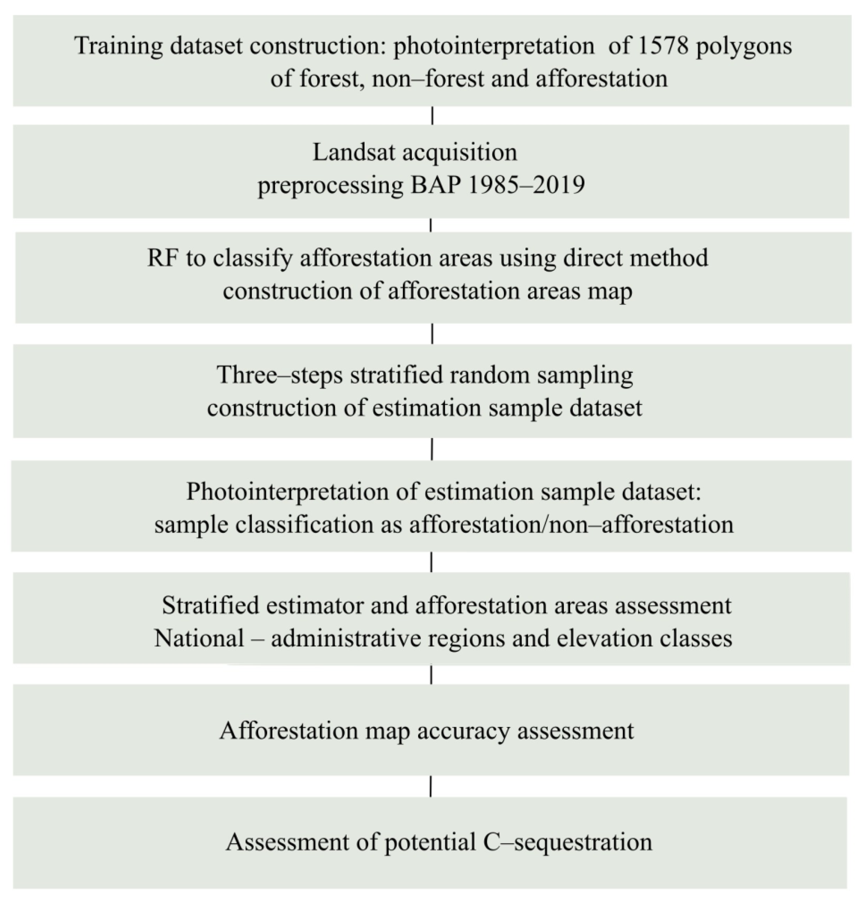Figure 2 illustrates the flowchart of the methods.

2.2.1. Afforestation Map Construction

RF Temporal Predictors

The six bands of the Landsat BAP composites acquired for each year between 1985 and 2019 were augmented with seven vegetation indices (VI): Normalized Difference Vegetation Index NDVI [54]; Normalized Burnt Ratio NBR [55]; Enhanced Vegetation Index EVI [56]; and Tasseled Cap Brightness B, Wetness W, Greeness G, and Angle A Indices [57]. The six bands together with the seven VIs comprised a dataset of 13 annual time series (TS) of 35 years of bands and indices. The bands and indices used to construct the TS were selected from among those considered in the literature to be the most useful for predicting forest changes [43].

Then, 18 temporal statistics were calculated for each TS of each polygon of the training dataset: mean, standard deviation, Kendall correlation [58], 11 percentiles from 0 to 100, mean of the first five years, mean of the last five years yearly minimum and yearly maximum. The result was a set of 234 temporal predictors (13 TS * 18 temporal statistics = 234 temporal predictors) which were used to calibrate the RF classification model, to directly predict afforestation areas in Italy and to construct the afforestation map via analyses of the trends of the temporal statistics linked to afforestation (A), non-forest (B), forest (C).

Random Forests

For classifying Italy into afforestation and non-afforestation areas, we used an RF model which was first calibrated using the training dataset and the associated BAP composite using the 234 temporal predictors, and then applied to Italy using the temporal predictors calculated for the rest of the BAP composite. Even though the RF algorithm accuracy is similar to accuracies for linear models, k-nearest neighbors [59,60], and more complex models such as neural networks, it was chosen because it can achieve large accuracy values as illustrated in [61,62] and because it is not excessively influenced by overfitting [20,63].

The RF hyperparameters can be calibrated to minimize error; two were calibrated for this study using a random search procedure [25,64]: (1) maximum features, the maximum number of temporal predictors considered and (2) maximum depth, the maximum depth of the tree, i.e., the longest path between the root node and the leaf node. For the random searches, we defined a grid of maximum features (1–52) and maximum depth (1–40) ranges, from which a subset of 100 combinations were randomly selected. The performance of each combination was assessed using k-fold cross validation (CV) with k = 5. Finally, the k-fold CV overall accuracy was calculated, and we selected the maximum features-maximum depth combination that produced the greatest accuracy. The number of trees in the algorithm was set to 500 and the minimum number of training sample units for splitting a node was set to one [25].

Finally, RF importance rankings were used to estimate the degree to which predictor variables contributed to increasing the accuracy of the map, to assess the most suitable variables for the classification model, and to verify their usefulness. The importance of the variables was calculated using the Mean Decrease Gini Index (MDG) which estimated the contribution of the variable to increasing the classification model accuracy. MDG is directly proportional to the contribution of the variable within the algorithm [65].

2.2.2. Selection of the Estimation Sample

To increase the precision of the afforestation area estimates and to increase the objectivity of the statistical inference from a sample [66], sample units were concentrated in the areas near the forest/non-forest map boundaries where classification errors were more likely. To this end, we used the forest/non-forest mask of Italy [38] described in Section 2.1.2. It was chosen because it has large accuracy (85%) and because as compared with other forest data (as Corine Land Cover and Corine Biotopes) it was the most accurate [39]. We resampled the forest mask to 30 m to be consistent with the afforestation map and to define a buffer of 120 m (four Landsat pixels) on each side of the forest/non-forest boundary to facilitate increasing the sampling intensity in the areas where classification errors were more likely [43]. The mean patch area of 11,104 m² and median of 1512 m² suggest that patches with centers near the forest/non-forest boundary are likely to be entirely within the 240 m total buffer width. By intersecting the buffer and the two classes of the afforestation map we obtained a map, hereafter designated the afforestation-buffer (AB) map, with four map classes: (i) afforestation inside the forest buffer, (ii) non-afforestation inside the forest buffer, (iii) afforestation outside the forest buffer, and (iv) non-afforestation outside the forest buffer.

Then, stratified random sampling with the four AB map classes serving as strata was implemented in three phases.

In the first phase, an initial random sample of points was selected from the four AB map classes, concentrating the larger number of points inside the forest buffer where the classification errors were more likely. A total of 2000 sample points was selected: 660 points were randomly selected in each of the afforestation and non-afforestation map classes inside the buffer, each representing 33% of the total sample, while 340 points were randomly selected in each of the afforestation and non-afforestation map classes outside the buffer, each representing 17% of the total sample.

These 2000 points were photointerpreted following a procedure similar to the procedure described for the training dataset using fine resolution imagery (Section 2.1.4). The photointerpretations were used to construct a confusion matrix for the afforestation/non-afforestation classification. Unlike the training dataset, for which the photointerpretation involved polygons, because the classification of BAP composite to construct the afforestation map is pixel based, the photointerpretation of the estimation sample dataset entailed classification of single Landsat pixels as afforestation or not afforestation. The matrix facilitates use of the stratified estimator described in Francini et al. [43] for estimating the afforestation area.

The second phase aimed at increasing the precision of the estimates. A second sample of 2000 points was selected with new within-class sample sizes proportional to the first phase within-class variance estimates: AB map classes with greater first-phase variances were sampled with greater intensities. In other words, in the second phase, more points were selected in the map classes with lower first-phase accuracies. The second phase distribution was 194 points in afforestation inside the forest buffer class, 835 points in non-afforestation inside the forest buffer class, 75 points in afforestation outside the forest buffer class, and 896 points in non-afforestation outside the forest buffer class. The second-phase sample was photointerpreted and the results were merged with the results of the first-phase sample photointerpretation, resulting in a total sample of 4000 points (

Table A1. Selection of first and second estimation sample dataset. The first estimation sample dataset composed of 2000 sample points. Per-class variance and resulting second sample selection. Through this procedure, the 2000 random points were selected in direct proportion to the variance of the first sample of points. At the end, the estimation sample dataset of 4000 points used for the next steps was extracted.

AB Map Class	Reference Class
	Afforestation	Non-Afforestation	First Sample Total	% Class Variances	Second Sample Total	Final Sample
afforestation inside buffer (i)	164	496	660	9.68	194	854
non-afforestation inside buffer (ii)	329	331	660	41.76	835	1495
afforestation outside buffer (iii)	9	331	340	3.75	75	415
non-afforestation outside buffer (iv)	26	314	340	44.80	896	1236
Total	528	1472	2000	100.00	2000	4000

in Appendix A). As for the first sample, a confusion matrix was constructed.

The third phase augmented the first and second phase samples to facilitate analyses of afforestation for (i) administrative regions and (ii) elevation classes. To align the administrative regions’ boundary shapefile and the DEM raster with the afforestation map, the boundary shapefile was rasterized at 30 m, while the DEM was resampled at 30 m and reclassified into 14 elevation classes (200 m intervals). The 20 administrative regions and the 14 elevation classes were intersected with the four AB map classes to produce a map with, respectively, 80 classes and 56 classes. Then, the 4000 points were assigned to their respective map classes obtained from the intersection of the four AB map classes and the administrative regions and the intersection of the four AB map classes and the elevation classes. The within-class samples were augmented with additional randomly selected points where necessary to obtain at least 30 points per class as a means of assuring reliable estimates of within-class variances.

The original estimation sample dataset of 4000 points was augmented as follows:

-

(i) For administrative region samples, we assigned the 4000 points to the 80 map classes obtained by intersecting the four AB map classes and the 20 administrative regions and augmented the samples for within-class estimation datasets that had fewer than 30 points. For this sample, we photointerpreted 254 additional points for a total of 4254 points.

-

(ii) For elevation class samples, we assigned the 4000 points to the 56 map classes obtained by intersecting the four AB map classes and the 14 elevation classes from the DEM and augmented the samples for within-class estimation datasets that had fewer than 30 points. For this sample, we photointerpreted 401 additional points for a total of 4401 points.

The two separate samples for the administrative regions and elevation classes were used to estimate afforestation areas inside and outside the forest buffer for each administrative region and each elevation class.

2.2.3. Accuracy Assessment and Afforestation Area Estimation

Using the estimation sample of size 4000, the stratified estimator was used to estimate overall accuracy (OA) and the national afforestation area. Then, we used the stratified estimators to estimate afforestation areas for each Italian administrative region using the estimation sample of size 2254 and, for each elevation class, using the estimation sample of size 4401. For individual administrative regions and for the national estimate over administrative regions, we used the stratified estimation with intersections of the 20 administrative regions and the four AB map classes as strata. In the same way, for individual elevation classes and for the national estimate over elevation classes, we used the stratified estimation with intersections of the 14 elevation classes and the four AB map classes as strata.

Following the photointerpretation, similar to that of the first phase (Section 2.1), the confusion matrices for administrative regions and elevation classes were constructed and used with the stratified estimator (

Table 1. Stratified estimator, confusion matrix to area estimates and CI width.

Map Class	Reference Class		Sum	${\mathrm{w}}_{\mathrm{j}}$#1	${\widehat{\mathrm{p}}}_{\mathrm{j}}$	${\mathrm{w}}_{\mathrm{j}}\ast {\widehat{\mathrm{p}}}_{\mathrm{j}}$	$\widehat{\mathrm{Var}}({\widehat{\mathrm{p}}}_{\mathrm{j}})$	${\mathrm{w}}_{\mathrm{j}}^2\ast \widehat{\mathrm{Var}}({\widehat{\mathrm{p}}}_{\mathrm{j}})$
	Afforest- Ation	Non- Afforest- Ation
Afforestation outside buffer	$n_{11}$	$n_{12}$	$n_1=n_{11}+n_{12}$	$w_1$	${\widehat{p}}_1=\frac{n_{11}}{n_1}$	$w_1\ast {\widehat{p}}_1$	$\widehat{Var}({\widehat{p}}_1)=\frac{{\widehat{p}}_1\ast \left(1-{\widehat{p}}_1\right)}{n_1}$	$w_1^2\ast \widehat{Var}({\widehat{p}}_1)$
Afforestation inside buffer	$n_{21}$	$n_{22}$	$n_2=n_{21}+n_{22}$	$w_2$	${\widehat{p}}_2=\frac{n_{21}}{n_2}$	$w_2\ast {\widehat{p}}_2$	$\widehat{Var}({\widehat{p}}_2)=\frac{{\widehat{p}}_2\ast \left(1-{\widehat{p}}_2\right)}{n_2}$	$w_2^2\ast \widehat{Var}({\widehat{p}}_2)$
Non-afforestation outside buffer	$n_{31}$	$n_{32}$	$n_3=n_{31}+n_{32}$	$w_3$	${\widehat{p}}_3=\frac{n_{31}}{n_3}$	$w_3\ast {\widehat{p}}_3$	$\widehat{Var}({\widehat{p}}_3)=\frac{{\widehat{p}}_3\ast \left(1-{\widehat{p}}_3\right)}{n_3}$	$w_3^2\ast \widehat{Var}({\widehat{p}}_3)$
Non-afforestation inside buffer	$n_{41}$	$n_{42}$	$n_4=n_{41}+n_{42}$	$w_4$	${\widehat{p}}_4=\frac{n_{41}}{n_4}$	$w_4\ast {\widehat{p}}_4$	$\widehat{Var}({\widehat{p}}_4)=\frac{{\widehat{p}}_4\ast \left(1-{\widehat{p}}_4\right)}{n_4}$	$w_4^2\ast \widehat{Var}({\widehat{p}}_4)$
	$n_1$	$n_2$	$n={{\displaystyle \sum }}_j^n{n}_j$	${{\displaystyle \sum }}_j^4{w}_j=1$		$\widehat{p}={{\displaystyle \sum }}_{\mathrm{j}}^4{\mathrm{w}}_{\mathrm{j}}\ast {\widehat{\mathrm{p}}}_{\mathrm{j}}{}^{ \#2}$		$\widehat{Var}\left(\widehat{p}\right)={\sum }_j^4{w}_j^2\ast \widehat{Var}\left({\widehat{p}}_j\right)$#3

^#1$w_{j }$ is the proportion of the map in each afforestation/non-afforestation inside/outside buffer class; ^#2 $\widehat{p}={\sum }_j^4{w}_j\ast {\widehat{p}}_j$ is the estimate of the proportion of the total area in one of the afforestation/non-afforestation inside/outside buffer classes; ^#3 $\widehat{Var}\left(\widehat{p}\right)={\sum }_j^4{w}_j^2\ast \widehat{Var }\left({\widehat{p}}_j\right)$ is the variance of the estimate of the total proportion of the area in one of the afforestation/non-afforestation inside/outside buffer classes [43].

). The area of afforestation that occurred between 1985 and 2019, was then estimated. The 95% confidence interval (CI) for the estimated area of each class was calculated following the estimator in Francini et al. [43], as illustrated in Table 1. Moreover, the stratified estimator is unbiased, meaning that the average of estimates over all possible samples of the same size obtained using the same sampling design equals the true value [36,43], although the estimate for any particular sample may deviate from the true value.

The national estimates were calculated by applying the stratified estimator to the confusion matrix for the map. For administrative regions, the intersection of the 20 administrative regions’ raster and the four AB map classes served as strata for the stratified estimator, and for the elevation classes, the intersection of the 14 elevation classes from the DEM raster and the four AB map classes from the afforestation map served as strata for the stratified estimator.

2.2.4. Potential Carbon Sequestration

To estimate the potential carbon that would be sequestered in areas predicted to be afforested between 1985 and 2019 once the forest had matured, we used the estimates of total biomass per unit of forest area over all pools (aboveground biomass, belowground biomass, litter, necromass, and organic and mineral soil) from the National Inventory of Forests and Carbon Sinks [67] for individual administrative regions [37]. For each region, we multiplied the estimated area of afforestation by the INFC estimate of biomass per unit area to obtain an estimate of total biomass once the forest is mature.

To estimate the potential C-sequestration (t), we multiplied the estimate of total biomass by the default carbon fraction in biomass of 0.5 [68,69]. The 95% confidence interval estimates were also calculated for the carbon estimates at the national and administrative region levels; as we did for the potential C-sequestration estimate, we multiplied the CI of the afforestation estimates (ha) and the total carbon stock (t/ha) given by the national forest inventory, and then we multiplied the total biomass CI (t) and the default carbon fraction of 0.5. It is important to emphasize that this estimate was affected by increased uncertainty due to the error associated with the INFC per unit area biomass estimates (SE is linked to the carbon pools and, at the national level, the aboveground biomass, belowground biomass, litter, necromass, and organic and mineral soil SE is about 1.4%) and the assumption of a common biomass to carbon conversion factor.

3. Results

3.1. Afforestation Map

The afforestation map (Figure 3) predicted two classes of land cover: afforestation between 1985 and 2019 and non-afforestation between 1985 and 2019. The afforestation map was intersected with the forest map buffer of 120 m (Section 2.2.2) to obtain the four AB map classes used to assess map accuracy and to estimate afforestation areas.

3.2. Accuracy Assessment

The estimated map OA was 87% with estimated afforestation classification accuracy of 49% inside the forest buffer class and 26% outside the buffer class. Non-afforestation classification accuracy estimates were larger both inside and outside the forest buffer, reaching 90% or greater (

Table A2. Overall accuracy assessment for the map. The table shows the overall and the class accuracies for the map, estimated from the confusion matrix and the sample of 4000 points.

AB Map Classes
	Reference		Total	Accuracy	Weight (Wt)	Wt *Acc
	Afforestation	Non-Afforestation
afforestation inside buffer (i)	418	436	854	0.49	0.11	0.05
non-afforestation inside buffer (ii)	60	1115	1175	0.95	0.30	0.29
afforestation outside buffer (iii)	191	544	735	0.26	0.08	0.02
non-afforestation outside buffer (iv)	16	1220	1236	0.99	0.52	0.51
Overall Accuracy						0.87

in Appendix B).

3.3. Area Estimates

Afforestation did not occur uniformly at the national level; in fact, when considering administrative region boundaries (Figure 4A,A1), estimates of afforestation areas for four administrative regions (Abruzzo, Calabria, Latium, and Sardinia) were greater than 200,000 ha, with the greatest estimate of 260,653 ± 58,522 ha (10.80% of the administrative region area) for Sardinia. Estimates were less than 90,000 ha for Apulia, Friuli Venezia Giulia, Molise, Valle d’Aosta, and Veneto, with the lowest estimate of 28,644 ± 12,114 ha (8.78% of the administrative region area) for Valle d’Aosta. In the remaining administrative regions, the estimated afforestation areas were between 100,000 and 200,000 ha (

Table A3. Stratified area estimates for Italian administrative regions. This table shows the afforestation estimates for each Italian administrative region in ha and percentage, with the associated standard error and 95% confidence interval width.

Administrative Region	Afforestation (ha)	Afforestation (%)	SE (ha)	SE (%)	CI Width (ha)	CI Width (%)
Abruzzo	218,839	20.27	23,035	10.53	46,071	21.05
Apulia	61,313	3.17	11,254	18.36	22,509	36.71
Basilicata	142,766	14.29	22,028	15.43	44,057	30.86
Calabria	222,525	14.75	27,302	12.27	54,604	24.54
Campania	151,133	11.11	24,805	16.41	49,610	32.83
Emilia-Romagna	183,743	8.19	26,858	14.62	53,716	29.23
Friuli Venezia Giulia	64,950	8.20	10,864	16.73	21,727	33.45
Latium	217,336	12.63	31,482	14.49	62,964	28.97
Liguria	108,395	20.00	15,639	14.43	31,277	28.85
Lombardy	129,382	5.42	17,173	13.27	34,346	26.55
Marche	120,337	12.82	15,784	13.12	31,569	26.23
Molise	74,489	16.78	12,987	17.44	25,975	34.87
Piedmont	187,841	7.40	26,166	13.93	52,333	27.86
Sardinia	260,653	10.81	29,261	11.23	58,522	22.45
Sicily	183,561	7.14	27,181	14.81	54,361	29.61
Trentino-Alto Adige	136,171	10.01	22,885	16.81	45,771	33.61
Tuscany	169,211	7.36	26,327	15.56	52,653	31.12
Umbria	104,304	12.34	18,450	17.69	36,900	35.38
Valle d’Aosta	28,644	8.78	6057	21.15	12,114	42.29
Veneto	89,398	4.88	21,365	23.90	42,731	47.80
National	2,855,009	9.53	98,087	3.44	196,175	6.87

in Appendix C). Abruzzo and Liguria had the greatest percentage afforestation estimates relative to the administrative region area.

The estimated afforestation area estimates for the elevation classes and at the national level are illustrated in Figure 4B,B1 and

Table A4. Stratified area estimates for elevation classes. This table shows the afforestation estimates for each elevation class in ha and percentage, with the associated standard error and 95% confidence interval width.

Elevation Classes	Afforestation (ha)	Afforestation (%)	SE (ha)	SE (%)	CI Width (ha)	CI Width (%)
<200	359,769	3.37	37,499	10.42	74,998	20.85
200–400	498,396	8.20	40,165	8.06	80,330	16.12
400–600	549,497	13.94	42,489	7.73	84,979	15.46
600–800	468,891	17.49	39,854	8.50	79,708	17.00
800–1000	354,437	19.55	37,065	10.46	74,131	20.92
1000–1200	226,546	18.53	29,391	12.97	58,782	25.95
1200–1400	94,722	10.56	11,994	12.66	23,988	25.33
1400–1600	101,565	15.18	20,946	20.62	41,891	41.25
1600–1800	64,805	12.55	12,066	18.62	24,133	37.24
1800–2000	47,693	11.26	10,289	21.57	20,578	43.15
2000–2200	55,295	16.01	10,420	18.84	20,841	37.69
2200–2400	16,226	5.92	3620	22.31	7240	44.62
>2400	474	0.11	441	93.14	883	186.27
National	2,801,050	9.35	94,647	3.38	189,293	6.76

in Appendix C. The largest afforestation area between 1985 and 2019 was estimated in the intermediate elevation classes. Below 1200 m a.s.l., estimates were greater than 200,000 ha, with the greatest estimate of 549,497 ± 84,979 ha (13.94%) for the 400–600 m a.s.l. class. For higher altitudes, estimates were less than 100,000 ha, a finding that aligns with the decrease in forest habitats. The greatest percentage afforestation area estimate was about 20.00% for the 600–1200 m a.s.l. class.

With the final estimation sample dataset, we estimated the national afforestation area using the stratified estimator three ways, each with a different set of map classes serving as strata: the four original AB map classes, the 80 classes obtained by intersecting the four AB map classes and the 20 administrative regions, and the 56 classes obtained by intersecting the four AB map classes and the 14 elevation classes. As expected, because the stratified estimator is unbiased and also because the estimates are based on the same afforestation map and on a common estimation sample, all three national estimates for the period 1985–2019 were very similar, approximately 2.8 ± 0.2 million ha, as shown in

Table 2. National afforestation area estimates.

	Area (ha)	SE (ha)	SE (%)	CI Width (ha)	CI Width (%)
National map	2,833,365	101,125	3.57	202,250	7.14
Elevation classes	2,801,050	94,647	3.38	189,293	6.76
Administrative regions	2,855,009	98,087	3.43	196,175	6.87

.

3.4. C-Sequestration Assessment

Considering administrative regions (Figure 5,

Table A5. Potential C-sequestration (t) and CI width (t) estimated in administrative regions in afforestation areas between 1985 and 2019.

Administrative Region	Afforestation(ha)	AfforestationCI Width (ha)	Total Biomass Stock (t/ha)	Afforestation Potential Biomass (t)	Potential C(t)	Potential Biomass CI Width(t)	Potential C CI Width (t)
Calabria	222,525	54,604	157.10	34,958,678	17,479,339	8,578,288	4,289,144
Abruzzo	218,839	46,071	140.00	30,637,460	15,318,730	6,449,940	3,224,970
Latium	217,336	62,964	135.40	29,427,294	14,713,647	8,525,326	4,262,663
Sardinia	260,653	58,522	99.50	25,934,974	12,967,487	5,822,939	2,911,470
Emilia-Romagna	183,743	53,716	140.00	25,724,020	12,862,010	7,520,240	3,760,120
Piedmont	187,841	52,333	136.70	25,677,865	12,838,932	7,153,921	3,576,961
Trentino-Alto Adige	136,171	45,771	181.30	24,687,802	12,343,901	8,298,282	4,149,141
Sicily	183,561	54,361	133.30	24,468,681	12,234,341	7,246,321	3,623,161
Campania	151,133	49,610	158.30	23,924,354	11,962,177	7,853,263	3,926,632
Tuscany	169,211	52,653	130.60	22,098,957	11,049,478	6,876,482	3,438,241
Lombardy	129,382	34,346	160.50	20,765,811	10,382,906	5,512,533	2,756,267
Basilicata	142,766	44,057	135.60	19,359,070	9,679,535	5,974,129	2,987,065
Marche	120,337	31,569	131.20	15,788,214	7,894,107	4,141,853	2,070,926
Liguria	108,395	31,277	131.40	14,243,103	7,121,552	4,109,798	2,054,899
Veneto	89,398	42,731	158.70	14,187,463	7,093,731	6,781,410	3,390,705
Umbria	104,304	36,900	121.50	12,672,936	6,336,468	4,483,350	2,241,675
Molise	74,489	25,975	155.60	11,590,488	5,795,244	4,041,710	2,020,855
Friuli Venezia Giulia	64,950	21,727	159.30	10,346,535	5,173,268	3,461,111	1,730,556
Apulia	61,313	22,509	138.20	8,473,457	4,236,728	3,110,744	1,555,372
Valle d’Aosta	28,644	12,114	102.50	2,936,010	1,468,005	1,241,685	620,843
Italy	2,855,009	196,175	141.80	404,840,276	202,420,138	27,817,615	13,908,808

in Appendix E), the region with the largest estimate of potential sequestered carbon was Calabria with 17,479,338 ± 4,289,144 t, while the region with the smallest estimate of potential carbon sequestrated was Valle d’Aosta with 1,468,005 ± 620,842 t. In 11 of the 20 administrative regions, estimates were greater than 10 million t of potential carbon sequestrated, and nationwide, 202,420,138 ± 13,908,807 t of potential carbon would be sequestrated when the trees in the afforestation areas mature.

4. Discussion

Afforestation processes can be natural via spontaneous colonization of vegetation succession or anthropogenic through planting or direct sowing. Afforestation is a profound and potentially long-lasting land use transformation that has implications for ecosystems and their associated services. It is, therefore, extremely important to monitor afforestation and to locate its occurrence as a means of facilitating development of effective and timely management plans.

4.1. Random Forest for Afforestation Map Construction

Using the RF model with the Landsat BAP composite (spatial resolution 30 m) data, we constructed a map that predicted areas in Italy where afforestation occurred between 1985 and 2019. Implementation of the classification method on GEE produced the afforestation map for the entirety of Italy in about three hours. The methodology is based on the use of Landsat BAP composites because their long historical series facilitates the prediction of slow phenomena such as afforestation. In addition, the use of multiple temporal predictors produced large accuracy estimates. Afforestation classification focused on mapping and predicting the area where afforestation had occurred in the past 35 years, as opposed to the exact year in which the forest was established which involves considering many different variables such as the forest type, elevation, latitude, and aspect.

Finally, the analysis of the importance of the variables (illustrated in Figure A1 and Figure A2 in Appendix D) used in the RF model allowed us to identify the variables that contributed most to the classification, thus, reducing the number of variables and speeding up classification operations. A variable with a greater weight in the classification means that it more accurately distinguishes among the afforestation/non-afforestation classes considered.

The most important predictor in the RF model was Kendall’s correlation (tau) of several bands and indices (mean value MDG > 8) and also the average of the values of several bands and indices (mean value MDG > 1). The predictor variables that had the greatest weight in the algorithm were Swir2 tau (MDG = 15.22), Swir1 tau (MDG = 14.79), TCW, and green band tau (MDG = 13.60).

4.2. Afforestation Map Validation and Accuracy Assessment

The validation of the map was carried out in two phases. A qualitative phase involved the visual analysis of the map and identified the major issues in the mapping process such as afforestation of agricultural areas including orchards, agroforestry and olive groves planted during the observation period, or even trees planted in urban areas. However, the visual analysis also made it possible to observe the accuracy with which the map predicted areas of afforestation due to agricultural abandonment or movement of the tree line to higher altitudes, as well as areas of afforestation, which involved many reforestations.

In the second stage of validation, we estimated the OA = 87%. The estimates of accuracies for the individual classes were quite large in non-afforestation classes (>95%) and smaller for the afforestation class outside the forest buffer where the accuracy was 26%, and 50% for the afforestation class inside buffer; this difference is probably due to the fact that outside the forest buffer the classification method was more influenced by the spectral response of other land cover types such as agricultural areas that can have similar spectral responses as afforestation. These results confirm the utility of constructing the 120 m buffer to increase the precision of the estimates. As before, increasing the sampling intensity where classification errors are more likely and area variance estimates are larger increases the precision of the estimates. Accordingly, we concentrated 18% of points in the class with accuracy 26%, 21% of points in the class with accuracy 49%, and 15% of points in each of the two classes with accuracies >90% (the two non-afforestation classes).

The map has some systematic commission errors, including agricultural areas, some urban areas, and linear elements such as roads. In general, agricultural areas are most prone to these errors. We have observed this feature in other maps and attribute it to crop variability which is subject to periodic cycles of growth. This error is also present in the afforestation inside the forest buffer class which could explain the smaller accuracies for classes inside the buffer as compared with those outside the buffer.

Map errors can also be traced back to the input data. Although the Landsat images have the advantage of a long time series, they can be affected by the diversity of the sensors mounted on different satellites which, in turn, can influence the output of the classification. The analysis of accuracy is important for focusing future research on the classes that have smaller accuracies, looking for an effective method to increase it.

4.3. Afforestation Area Estimates

The statistically rigorous, unbiased stratified estimator resulted in more precise estimates of the afforestation areas. The intermediate result based on the first-phase sample of 2000 random points showed that predicted afforestation between 1985 and 2019 covered 3,273,496 ± 401,557 ha. Following the second-phase sample which produced a total of 4000 random points, the estimate of the area subject to afforestation was 2,833,365 ± 202,250 ha. With the final sample, the area of afforestation between 1985 and 2019 was estimated to be 2,801,050 ± 189,293 ha when using the intersection of the 14 elevation classes and four AB map classes as strata, and 2,855,009 ± 196,175 ha when using the intersection of the 20 administrative regions and the four AB map classes as strata, or an average of ±82,000 ha per year (0.3% of the national area). It is important to note that the increase in the sample size reduced the estimates of the variances and SEs. Overall, all the estimates are reliable, and the SEs are similar and small (from 3.30 to 3.50%), moreover the estimate for any estimate is included in the CIs for the other estimates, e.g., the CI of the national afforestation estimate assessed using elevation classes (189,239 ha) and administrative regions (196,175 ha) are included in the CI of the national afforestation (202,250 ha). Confidence interval widths as percentages of the estimates were between 6.76% for the elevation classes, 6.87% for the administrative regions, and 7.14% for the national map.

Afforestation estimates at the national level corresponded well with results from the National Inventory of Forests and Carbon Sinks (INFC) which estimated an annual percentage increase of 0.2–0.3% in the national area, equal to approximately 77,960 ha between 1985 and 2005 and 52,856 ha between 2005–2015 [37]. The estimates for this study and the INFC estimates are not completely comparable because the INFC estimates afforestation for forest and other wooded land following the FAO definition, whereas this study focused on the definition of afforestation proposed by FAO [2]. Nevertheless, the general comparability of the estimates lends credibility to them.

Studying afforestation within individual administrative regions and elevation classes was important because it facilitated assessment of afforestation in Italy in which it generally differs, not only in terms of the physical characteristics of the land, but also in terms of forest management systems. The DEM facilitates analyses of afforestation in the different elevation classes, and therefore, it is then possible to reflect on the forests and species most subject to afforestation.

The afforestation area estimates for the elevation classes showed that the greatest increase in area has been in deciduous or evergreen broadleaf forests at lower altitudes, while coniferous areas have expanded at higher altitudes. Above 1200 m, but below the tree line, afforestation has been less, so presumably, the expansion of coniferous forests such as Larix decidua has been less than in forests at lower altitudes.

The distribution of afforestation in the Italian administrative regions showed greater estimates in the southern regions, where an increase of 1,315,280 ha was estimated, while in the north and center the estimates were 928 ha and 611 ha, respectively.

These results can be attributed to agricultural abandonment which occurred at lower altitudes and in southern Italy which generally have fewer intensive forms of management than in center-north Italy where farms are more specialized.

In addition to INFC afforestation estimates, another result which is consistent with our afforestation results, was reported by Pompei [70] for Abruzzo, specifically that between 1954 and 2002 estimated afforestation areas covered almost 18% of the administrative region area with an annual percentage increase of 0.4%. These estimates corresponded to our estimates in which the estimate of afforestation area between 1985 and 2019 in Abruzzo covered 20% of the administrative region area with an annual percentage increase of 0.6%.

4.4. Potential C-Sequestration

Afforestation estimates were also used to estimate the potential C-sequestration in areas where afforestation occurred between 1985 and 2019. Potential C-sequestration refers to the amount of carbon (t) which would be absorbed by trees in the afforestation areas when they are mature. The estimates of the potential carbon sequestered in afforestation areas showed a slight decoupling between administrative region afforestation areas and the amount of carbon sequestered. In fact, while Sardinia had the greatest afforestation area, it was not the administrative region with the greatest amount of potential carbon sequestered. This is because carbon content in forests depends on different distributions of carbon in different forest pools, a result influenced both by climatic and geographic factors.

Considering the average 50-year age of Italian forests, it is important to note that because afforestation areas are not yet mature forests, our results illustrate the potential C-sequestration, therefore, the amount of carbon which a mature forest would sequester. To precisely assess the amount of C-sequestration, it would be important to know the forest age and other elements such as the geographical location, as well as the environmental and soil characteristics.

The large uncertainty in the potential C-sequestration estimates is due to the association of several errors arising from the uncertainty in the conversion of biomass to carbon which is used together with afforestation areas to approximately estimate the carbon from biomass values.

4.5. Future Developments

Afforestation is an extremely important environmental phenomenon. On the one hand, it is a topical issue and it is included in many international and national programs and legislation. On the other hand, afforestation mapping through remote sensing imagery analysis is still unexplored, very few studies have been reported, most of which have focused on small study areas [71].

The analysis of afforestation areas can be strengthened by improving the classification to decrease omission and commission errors using additional auxiliary data related to the afforestation process such as aspect, slope, pedology, and geographical area. The analysis of afforestation could also be useful for accurately predicting the vegetation associations and, therefore, the species that have been the protagonists of afforestation over the last 35 years, and for establishing the year when the afforestation process ended. This could also be useful to define a minimum time range in which afforestation could be estimated with consideration of the different growth rates for different species.

The method of afforestation classification can be the basis for studying afforestation dynamics. Future research can involve the classification method to assess many ecosystem services such as C-sequestration which can be estimated using both the classification method and chronosequences [72]. The classification method can be useful to predict where afforestation is occurring in support of ad hoc forest management strategies. Since the beginning of the 20th century until the 1970s, afforestation in Italy has occurred mainly by tree planting. Currently, afforestation in Italy is mostly via spontaneous vegetative succession [73], therefore, the classification method and the analysis of the afforestation spectral response can be adjusted to distinguish anthropogenic and natural afforestation. Finally, the classification method facilitates assessment of the rate of afforestation within elevation classes or ecoregions, and to characterize afforestation trends.

5. Conclusions

In this study, we constructed a 30 m map of afforestation areas that occurred between 1985 and 2019 using random forests and Landsat composite BAP data, and we estimated afforestation areas using the statistically rigorous stratified estimator. Three main conclusions were drawn from the study. Firstly, thanks to remotely sensed data with fine spatial resolution and available for long time series, it is possible to predict locations of afforestation areas by analyzing their evolution over time. Secondly, predicted afforestation maps can be integrated with a photointerpretation phase and auxiliary information such as administrative region boundaries and the DEM to facilitate analyses of territorial differences of the afforestation phenomenon, offering estimates that can be important from a management point of view. Finally, integration of the map with sample data in combination with the statistically rigorous stratified estimators has shown that afforestation in Italy over the last 35 years has been about 2 million ha, associated with 202 million t of carbon sequestrated. The uncertainties of the results are relatively small, about 7.14% for the national estimates, 6.76% for the elevation classes, and 6.87% for the administrative regions, and these results confirm the effectiveness of the stratified estimator in increasing the accuracy of the estimates using an initial sample of points that is supplemented as needed. These results contribute to a greater understanding of the evolution of tree cover which is fundamental for monitoring climate change. For these reasons it will be important to strengthen the analysis and to improve the quality of the information that can be extracted from cartographic data in support of decision making.

References

- FAO. Global Forest Resources Assessment 2000 Main Report. Land Use Policy 2003, 20, 195. [Google Scholar] [CrossRef]
- FAO. Global Forest Resources Assessment 2020 Main Report; FAO: Rome, Italy, 2020. [Google Scholar]
- Spadoni, G.L.; Cavalli, A.; Congedo, L.; Munafò, M. Analysis of Normalized Difference Vegetation Index (NDVI) Multi-Temporal Series for the Production of Forest Cartography. Remote Sens. Appl. 2020, 20, 100419. [Google Scholar] [CrossRef]
- Intergovernmental Panel on Climate Change Agriculture, Forestry and Other Land Use (AFOLU). Climate Change 2014 Mitigation of Climate Change; Cambridge University Press: Cambridge, UK, 2015; pp. 811–922. [Google Scholar] [CrossRef]
- Shukla, P.R.; Skea, J.; Slade, R.; van Diemen, R.; Haughey, E.; Malley, J.; Pathak, M.; Pereira, J.P. Foreword Technical and Preface. In Climate Change and Land: An IPCC Special Report on Climate Change, Desertification, Land Degradation, Sustainable Land Management, Food Security, and Greenhouse Gas Fluxes in Terrestrial Ecosystems; Cambridge University Press: Cambridge, UK, 2019; pp. 35–74. [Google Scholar]
- Buscardo, E.; Smith, G.F.; Kelly, D.L.; Freitas, H.; Iremonger, S.; Mitchell, F.J.G.; O’Donoghue, S.; McKee, A.M. The Early Effects of Afforestation on Biodiversity of Grasslands in Ireland. Biodivers. Conserv. 2008, 17, 1057–1072. [Google Scholar] [CrossRef]
- Veldman, J.W.; Overbeck, G.E.; Negreiros, D.; Mahy, G.; le Stradic, S.; Fernandes, G.W.; Durigan, G.; Buisson, E.; Putz, F.E.; Bond, W.J. Where Tree Planting and Forest Expansion Are Bad for Biodiversity and Ecosystem Services. Bioscience 2015, 65, 1011–1018. [Google Scholar] [CrossRef]
- Chersich, S.; Rejšek, K.; Vranová, V.; Bordoni, M.; Meisina, C. Climate Change Impacts on the Alpine Ecosystem: An Overview with Focus on the Soil—A Review. J. For. Sci. 2015, 61, 496–514. [Google Scholar] [CrossRef]
- European Commission. New EU Forest Strategy for 2030; COM(2021) 572 final; European Commission: Brussels, Belgium, 2021. [Google Scholar]
- MIPAAF. Strategia Forestale Nazionale; MIPAAF: Rome, Italy, 2018. [Google Scholar]
- Nabuurs, G.-J.; Harris, N.; Sheil, D.; Palahi, M.; Chirici, G.; Boissière, M.; Fay, C.; Reiche, J.; Valbuena, R. Glasgow Forest Declaration Needs New Modes of Data Ownership. Nat. Clim. Change 2022, 12, 415–417. [Google Scholar] [CrossRef]
- Francini, S.; Chirici, G. A Sentinel-2 Derived Dataset of Forest Disturbances Occurred in Italy between 2017 and 2020. Data Brief 2022, 42, 108297. [Google Scholar] [CrossRef]
- Wulder, M.A.; Coops, N.C. Satellites: Make Earth Observations Open Access. Nature 2014, 513, 30–31. [Google Scholar] [CrossRef]
- Gorelick, N.; Hancher, M.; Dixon, M.; Ilyushchenko, S.; Thau, D.; Moore, R. Google Earth Engine: Planetary-Scale Geospatial Analysis for Everyone. Remote Sens. Environ. 2017, 202, 18–27. [Google Scholar] [CrossRef]
- McRoberts, R.E.; Næsset, E.; Gobakken, T.; Bollandsås, O.M. Indirect and Direct Estimation of Forest Biomass Change Using Forest Inventory and Airborne Laser Scanning Data. Remote Sens. Environ. 2015, 164, 36–42. [Google Scholar] [CrossRef]
- Fuller, R.M.; Smith, G.M.; Devereux, B.J. The Characterisation and Measurement of Land Cover Change through Remote Sensing: Problems in Operational Applications? Int. J. Appl. Earth Obs. Geoinf. 2003, 4, 243–253. [Google Scholar] [CrossRef]
- Bollandsås, O.M.; Gregoire, T.G.; Næsset, E.; Øyen, B.H. Detection of Biomass Change in a Norwegian Mountain Forest Area Using Small Footprint Airborne Laser Scanner Data. Stat. Methods Appl. 2013, 22, 113–129. [Google Scholar] [CrossRef]
- Skowronski, N.S.; Clark, K.L.; Gallagher, M.; Birdsey, R.A.; Hom, J.L. Airborne Laser Scanner-Assisted Estimation of Aboveground Biomass Change in a Temperate Oak-Pine Forest. Remote Sens. Environ. 2014, 151, 166–174. [Google Scholar] [CrossRef]
- Breiman, L. Random Forest. Mach. Learn. 2001, 45, 5–32. [Google Scholar] [CrossRef]
- Belgiu, M.; Drăgu, L. Random Forest in Remote Sensing: A Review of Applications and Future Directions. ISPRS J. Photogramm. Remote Sens. 2016, 114, 24–31. [Google Scholar] [CrossRef]
- Kennedy, R.E.; Yang, Z.; Cohen, W.B. Detecting Trends in Forest Disturbance and Recovery Using Yearly Landsat Time Series: 1. LandTrendr-Temporal Segmentation Algorithms. Remote Sens. Environ. 2010, 114, 2897–2910. [Google Scholar] [CrossRef]
- Hansen, M.C.; Potapov, P.V.; Moore, R.; Hancher, M.; Turubanova, S.A.; Tyukavina, A.; Thau, D.; Stehman, S.V.; Goetz, S.J.; Loveland, T.R.; et al. High-Resolution Global Maps of 21st-Century Forest Cover Change. Science 2013, 342, 850–853. [Google Scholar] [CrossRef]
- Coops, N.C.; Shang, C.; Wulder, M.A.; White, J.C.; Hermosilla, T. Change in Forest Condition: Characterizing Non-Stand Replacing Disturbances Using Time Series Satellite Imagery. For. Ecol. Manag. 2020, 474, 118370. [Google Scholar] [CrossRef]
- Murillo-Sandoval, P.J.; van Dexter, K.; van den Hoek, J.; Wrathall, D.; Kennedy, R. The End of Gunpoint Conservation: Forest Disturbance after the Colombian Peace Agreement. Environ. Res. Lett. 2020, 15, 34033. [Google Scholar] [CrossRef]
- Laurin, G.V.; Francini, S.; Luti, T.; Chirici, G.; Pirotti, F.; Papale, D. Satellite Open Data to Monitor Forest Damage Caused by Extreme Climate-Induced Events: A Case Study of the Vaia Storm in Northern Italy. Forestry 2021, 94, 407–416. [Google Scholar] [CrossRef]
- Qiu, B.; Zou, F.; Chen, C.; Tang, Z.; Zhong, J.; Yan, X. Automatic Mapping Afforestation, Cropland Reclamation and Variations in Cropping Intensity in Central East China during 2001–2016. Ecol. Indic. 2018, 91, 490–502. [Google Scholar] [CrossRef]
- Yin, H.; Pflugmacher, D.; Li, A.; Li, Z.; Hostert, P. Land Use and Land Cover Change in Inner Mongolia-Understanding the Effects of China’s Re-Vegetation Programs. Remote Sens. Environ. 2018, 204, 918–930. [Google Scholar] [CrossRef]
- Ramírez-Cuesta, J.M.; Minacapilli, M.; Motisi, A.; Consoli, S.; Intrigliolo, D.S.; Vanella, D. Characterization of the Main Land Processes Occurring in Europe (2000–2018) through a MODIS NDVI Seasonal Parameter-Based Procedure. Sci. Total Environ. 2021, 799, 149346. [Google Scholar] [CrossRef] [PubMed]
- Zhu, Z.; Woodcock, C.E. Continuous Change Detection and Classification of Land Cover Using All Available Landsat Data. Remote Sens. Environ. 2014, 144, 152–171. [Google Scholar] [CrossRef]
- Huang, H.; Chen, Y.; Clinton, N.; Wang, J.; Wang, X.; Liu, C.; Gong, P.; Yang, J.; Bai, Y.; Zheng, Y.; et al. Mapping Major Land Cover Dynamics in Beijing Using All Landsat Images in Google Earth Engine. Remote Sens. Environ. 2017, 202, 166–176. [Google Scholar] [CrossRef]
- Luti, T.; de Fioravante, P.; Marinosci, I.; Strollo, A.; Riitano, N.; Falanga, V.; Mariani, L.; Congedo, L.; Munafò, M. Land Consumption Monitoring with Sar Data and Multispectral Indices. Remote Sens. 2021, 13, 1586. [Google Scholar] [CrossRef]
- Chirici, G.; Giannetti, F.; Mazza, E.; Francini, S.; Travaglini, D.; Pegna, R.; White, J.C. Monitoring Clearcutting and Subsequent Rapid Recovery in Mediterranean Coppice Forests with Landsat Time Series. Ann. For. Sci. 2020, 77, 40. [Google Scholar] [CrossRef]
- Olofsson, P.; Foody, G.M.; Stehman, S.V.; Woodcock, C.E. Making Better Use of Accuracy Data in Land Change Studies: Estimating Accuracy and Area and Quantifying Uncertainty Using Stratified Estimation. Remote Sens. Environ. 2013, 129, 122–131. [Google Scholar] [CrossRef]
- Olofsson, P.; Foody, G.M.; Herold, M.; Stehman, S.V.; Woodcock, C.E.; Wulder, M.A. Good Practices for Estimating Area and Assessing Accuracy of Land Change. Remote Sens. Environ. 2014, 148, 42–57. [Google Scholar] [CrossRef]
- Marcelli, A.; Mattioli, W.; Puletti, N.; Chianucci, F.; Gianelle, D.; Grotti, M.; Chirici, G.; D’Amico, G.; Francini, S.; Travaglini, D.; et al. Large-Scale Two-Phase Estimation of Wood Production by Poplar Plantations Exploiting Sentinel-2 Data as Auxiliary Information. Silva Fenn. 2020, 54, 1–15. [Google Scholar] [CrossRef]
- Wagner, J.E.; Stehman, S.V. Optimizing Sample Size Allocation to Strata for Estimating Area and Map Accuracy. Remote Sens. Environ. 2015, 168, 126–133. [Google Scholar] [CrossRef]
- RAF. RaFITALIA 2017–2018. In Rapporto Sullo Stato Delle Foreste e del Settore Forestale in Italia; Compagnia delle Foreste S.R.L.: Arezzo, Italy, 2019; ISBN 978-88-98850-34-1. [Google Scholar]
- D’amico, G.; Vangi, E.; Francini, S.; Giannetti, F.; Nicolaci, A.; Travaglini, D.; Massai, L.; Giambastiani, Y.; Terranova, C.; Chirici, G. Are We Ready for a National Forest Information System? State of the Art of Forest Maps and Airborne Laser Scanning Data Availability in Italy. IForest 2021, 14, 144–154. [Google Scholar] [CrossRef]
- Vangi, E.; D’amico, G.; Francini, S.; Giannetti, F.; Lasserre, B.; Marchetti, M.; McRoberts, R.E.; Chirici, G. The Effect of Forest Mask Quality in the Wall-to-wall Estimation of Growing Stock Volume. Remote Sens. 2021, 13, 1038. [Google Scholar] [CrossRef]
- ISTAT. Descrizione dei Dati Geografici dei Confini Delle Unità Amministrative a Fini Statistici; ISTAT: Rome, Italy, 2019. [Google Scholar]
- Tarquini, S.; Isola, I.; Favalli, M.; Mazzarini, F.; Bisson, M.; Pareschi, M.T.; Boschi, E. TINITALY/01: A New Triangular Irregular Network of Italy. Ann. Geophys. 2009, 50, 407–425. [Google Scholar] [CrossRef]
- Tarquini, S.; Vinci, S.; Favalli, M.; Doumaz, F.; Fornaciai, A.; Nannipieri, L. Release of a 10-m-Resolution DEM for the Italian Territory: Comparison with Global-Coverage DEMs and Anaglyph-Mode Exploration via the Web. Comput. Geosci. 2012, 38, 168–170. [Google Scholar] [CrossRef]
- Francini, S.; McRoberts, R.E.; D’Amico, G.; Coops, N.C.; Hermosilla, T.; White, J.C.; Wulder, M.A.; Marchetti, M.; Mugnozza, G.S.; Chirici, G. An Open Science and Open Data Approach for the Statistically Robust Estimation of Forest Disturbance Areas. Int. J. Appl. Earth Obs. Geoinf. 2022, 106, 102663. [Google Scholar] [CrossRef]
- Gomes, V.C.F.; Queiroz, G.R.; Ferreira, K.R. An Overview of Platforms for Big Earth Observation Data Management and Analysis. Remote Sens. 2020, 12, 1253. [Google Scholar] [CrossRef]
- White, J.C.; Wulder, M.A.; Hobart, G.W.; Luther, J.E.; Hermosilla, T.; Griffiths, P.; Coops, N.C.; Hall, R.J.; Hostert, P.; Dyk, A.; et al. Pixel-Based Image Compositing for Large-Area Dense Time Series Applications and Science. Can. J. Remote Sens. 2014, 40, 192–212. [Google Scholar] [CrossRef]
- White, J.C.; Wulder, M.A.; Hermosilla, T.; Coops, N.C.; Hobart, G.W. A Nationwide Annual Characterization of 25 Years of Forest Disturbance and Recovery for Canada Using Landsat Time Series. Remote Sens. Environ. 2017, 194, 303–321. [Google Scholar] [CrossRef]
- Griffiths, P.; van der Linden, S.; Kuemmerle, T.; Hostert, P. Erratum: A Pixel-Based Landsat Compositing Algorithm for Large Area Land Cover Mapping. IEEE J. Sel. Top. Appl. Earth Obs. Remote. Sens. 2013, 6, 2088–2101. [Google Scholar] [CrossRef]
- Hermosilla, T.; Wulder, M.A.; White, J.C.; Coops, N.C.; Hobart, G.W. An Integrated Landsat Time Series Protocol for Change Detection and Generation of Annual Gap-Free Surface Reflectance Composites. Remote Sens. Environ. 2015, 158, 220–234. [Google Scholar] [CrossRef]
- Hermosilla, T.; Wulder, M.A.; White, J.C.; Coops, N.C.; Hobart, G.W. Regional Detection, Characterization, and Attribution of Annual Forest Change from 1984 to 2012 Using Landsat-Derived Time-Series Metrics. Remote Sens. Environ. 2015, 170, 121–132. [Google Scholar] [CrossRef]
- Sallustio, L.; Munafò, M.; Riitano, N.; Lasserre, B.; Fattorini, L.; Marchetti, M. Integration of Land Use and Land Cover Inventories for Landscape Management and Planning in Italy. Environ. Monit. Assess. 2016, 188, 48. [Google Scholar] [CrossRef]
- Marchetti, M.; Bertani, R.; Corona, P.; Valentini, R. Changes of Forest Coverage and Land Uses as Assessed by the Inventory of Land Uses in Italy. For.@-Riv. Di Selvic. Ed Ecol. For. 2012, 9, 170–184. [Google Scholar] [CrossRef]
- Francini, S.; McRoberts, R.E.; Giannetti, F.; Marchetti, M.; Scarascia Mugnozza, G.; Chirici, G. The Three Indices Three Dimensions (3I3D) Algorithm: A New Method for Forest Disturbance Mapping and Area Estimation Based on Optical Remotely Sensed Imagery. Int. J. Remote Sens. 2021, 42, 4697–4715. [Google Scholar] [CrossRef]
- Francini, S.; Amico, G.D.; Vangi, E.; Borghi, C. Integrating GEDI and Landsat: Spaceborne Lidar and Four Decades of Optical Imagery for the Analysis of Forest Disturbances and Biomass Changes in Italy. Sensors 2022, 22, 2015. [Google Scholar] [CrossRef]
- Rouse, J.W., Jr.; Haas, R.H.; Deering, D.W.; Schell, J.A.; Harlan, J.C. Monitoring the Vernal Advancement and Retrogradation (Green Wave Effect) of Natural Vegetation, NASA/GSFC Type III Final Report 1974; Texas A&M University Remote Sensing Center: Greenbelt, MD, USA, 1973; 371p. [Google Scholar]
- Key, C.H.; Benson, N.C. Landscape Assessment (LA) Sampling and Analysis Methods. In USDA Forest Service-General Technical Report RMRS-GTR; USDA Forest Service, Rocky Mountain Research Station: Ogden, UT, USA, 2006. [Google Scholar]
- Huete, A.R. Modis vegetation index algorithm theoretical basis v3. Environ. Sci. 1999. [Google Scholar]
- Kauth, R.J. Tasselled Cap—A Graphic Description of the Spectral-Temporal Development of Agricultural Crops as Seen By Landsat; Purdue University: West Lafayette, IN, USA, 1976; pp. 41–51. [Google Scholar]
- Knight, W.R. A Computer Method for Calculating Kendall’s Tau with Ungrouped Data. J. Am. Stat. Assoc. 1966, 61, 436–439. [Google Scholar] [CrossRef]
- Tomppo, E. Satellite image based national forest inventory of Finland. Int. Arch. Photogramm. Remote Sens. 1991, 28, 419–424. [Google Scholar]
- Chirici, G.; Mura, M.; McInerney, D.; Py, N.; Tomppo, E.O.; Waser, L.T.; Travaglini, D.; McRoberts, R.E. A Meta-Analysis and Review of the Literature on the k-Nearest Neighbors Technique for Forestry Applications That Use Remotely Sensed Data. Remote Sens. Environ. 2016, 176, 282–294. [Google Scholar] [CrossRef]
- Nguyen, H.T.T.; Doan, T.M.; Tomppo, E.; McRoberts, R.E. Land Use/Land Cover Mapping Using Multitemporal Sentinel-2 Imagery and Four Classification. Remote Sens. 2020, 12, 1367. [Google Scholar] [CrossRef]
- Thanh Noi, P.; Kappas, M. Comparison of Random Forest, k-Nearest Neighbor, and Support Vector Machine Classifiers for Land Cover Classification Using Sentinel-2 Imagery. Sensors 2017, 18, 18. [Google Scholar] [CrossRef]
- Hawryło, P.; Francini, S.; Chirici, G.; Giannetti, F.; Parkitna, K.; Krok, G.; Mitelsztedt, K.; Lisańczuk, M.; Stereńczak, K.; Ciesielski, M.; et al. The Use of Remotely Sensed Data and Polish NFI Plots for Prediction of Growing Stock Volume Using Different Predictive Methods. Remote Sens. 2020, 12, 3331. [Google Scholar] [CrossRef]
- Bergstra, J.; Bengio, Y. Random Search for Hyper-Parameter Optimization. J. Mach. Learn. Res. 2012, 13, 281–305. [Google Scholar]
- Nicodemus, K.K. Letter to the Editor: On the Stability and Ranking of Predictors from Random Forest Variable Importance Measures. Brief. Bioinform. 2011, 12, 369–373. [Google Scholar] [CrossRef]
- Fattorini, L. Design-Based Methodological Advances to Support National Forest Inventories: A Review of Recent Proposals. IForest 2014, 8, 6–11. [Google Scholar] [CrossRef]
- INFC. Inventario Nazionale Delle Foreste e dei Serbatoi Forestali di Carbonio; Ministero delle Politiche Agricole Alimentari e Forestali, Ispettorato Generale-Corpo Forestale dello Stato-CRA-Unitò di ricerca per il monitoraggio e la Pianificazione forestale: Rome, Italy, 2005. [Google Scholar]
- Intergovernal Panel on Climate Change. Revised 1996 IPCC Guidelines for National Greenhouse Gas Emission Inventories. In Reference Manual, Reporting Guidelines and Workbook; Cambridge University Press: Cambridge, UK, 1997; Volume 3. [Google Scholar]
- Vitullo, M.; de Lauretis, R.; Federici, S. La Contabilità Del Carbonio Contenuto Nelle Foreste Italiane. Silvae 2008, 9, 91–104. [Google Scholar]
- Pompei, E. Espansione Delle Foreste Italiane Negi Ultimi 50 Anni: Il Caso Della Regione Abruzzo. Ph.D. Thesis, Tuscia University, Viterbo, WI, USA, 2007; p. 162. [Google Scholar]
- Ershov, D.V.; Gavrilyuk, E.A.; Koroleva, N.V.; Belova, E.I.; Tikhonova, E.V.; Shopina, O.V.; Titovets, A.V.; Tikhonov, G.N. Natural Afforestation on Abandoned Agricultural Lands during Post-Soviet Period: A Comparative Landsat Data Analysis of Bordering Regions in Russia and Belarus. Remote Sens. 2022, 14, 322. [Google Scholar] [CrossRef]
- Alberti, G.; Peressotti, A.; Piussi, P.; Zerbi, G. Forest Ecosystem Carbon Accumulation during a Secondary Succession in the Eastern Prealps of Italy. Forestry 2008, 81, 1–11. [Google Scholar] [CrossRef]
- Agnoletti, M.; Piras, F.; Venturi, M.; Santoro, A. Cultural Values and Forest Dynamics: The Italian Forests in the Last 150 Years. For. Ecol. Manag. 2022, 503, 119655. [Google Scholar] [CrossRef]