Article

Calibration of the ESA CCI-Combined Soil Moisture Products on the Qinghai-Tibet Plateau

1
School of Hydrology and Water Resources, Nanjing University of Information Science and Technology, Nanjing 210044, China
2
School of Environmental and Municipal Engineering, Lanzhou Jiaotong University, Lanzhou 730070, China
*
Author to whom correspondence should be addressed.
Remote Sens. 2023, 15(4), 918; https://doi.org/10.3390/rs15040918
Submission received: 23 November 2022 / Revised: 3 February 2023 / Accepted: 6 February 2023 / Published: 7 February 2023
(This article belongs to the Special Issue Remote Sensing and Land Surface Process Models for Permafrost Studies)

Abstract

:
Soil moisture (SM) retrieved from satellite and spaceborn sensors provides useful parameters for earth system models (ESMs). The Climate Change Initiative (CCI) SM products released by the European Space Agency have been widely used in many humid/semi-humid climatic regions due to their relatively long-term record. However, the performance of these products in cold and arid regions, such as the Qinghai-Tibetan Plateau (QTP), is largely unknown, necessitating urgent evaluation and calibration in these areas. In this work, we evaluated the reliability and improved the accuracy of the active-passive combined CCI products (CCI-C) using in-situ measured SM contents (SMC) under different underlying surface conditions. First, some conventional models were used to investigate the relationship between the CCI-C and the in-situ observed SMC, yielding similar fitting performances. Next, the random forest method and multiple linear regression were used to contrast the conventional models to calibrate and validate the CCI-C SM product based on the in-situ observed SMC, and the random forest method was found to have the highest accuracy. However, calibration of the CCI-C SM data with the best-performed random forest method based on different spatial zonation methods, e.g., by climate, topography, land cover, and vegetation, resulted in distinct spatial patterns of SM. Compared to a widely-used satellite SM product, namely the Soil Moisture Active Passive (SMAP) SM dataset, the calibrated CCI-C SM data based on climatic and vegetation zonation were larger but had similar spatial patterns. This study also points to the value of the calibrated CCI-C SM product to support land surface studies on the QTP.

1. Introduction

Near-surface soil moisture (SM) conditions influence the energy balance between the land surface and the atmosphere [1,2] by changing surface albedo and the partitioning of latent and sensible heat. SM also plays an important role in the water cycle, sediment transportation, and ecological succession [3]. Currently, there are three main methods to determine SM dynamics: field observation, remote sensing inversion, and model simulation. In many areas, field observation data are scarce due to the sparse distribution of observation sites. As a result, remote sensing inversion is a potentially useful method for obtaining SM data on a large scale. However, the remote sensing-acquired SM products should be evaluated against ground observation data [4] before they can be used for any SM-related studies or models [5]. For example, the Soil Moisture and Ocean Salinity (SMOS) products appear to be affected by radio frequency interference, resulting in large discrepancies from the ground truth [6]. The Soil Moisture Active Passive (SMAP) product performed well in barren land but tended to underestimate SM content (SMC) in cold regions and woody vegetative areas [7].
The Qinghai-Tibet Plateau (QTP), which occupies the largest permafrost zone in the mid- and low-latitudes, is highly sensitive to climate change [8,9]. Through interaction with the Asian monsoon and global atmospheric circulation, hydrological processes on the QTP have important impacts on the ecological environment and provide feedbacks to the climate system in China, Asia, and even around the globe [10,11]. Therefore, changes in SM conditions on the QTP have raised many concerns. From previous reports [12], SM conditions on the QTP were characterized by great heterogeneity on the land surface and substrates. In wet seasons, rainfall predominately controls SM dynamics, while temperature significantly affects SM in dry seasons [13]. These SM studies were mainly based on field observations representative of only small areas. For a region such as the QTP with a vast area, remote sensing-based time-series SM data become extremely important to understand the temporal and spatial dynamics and trends of change in SM [14].
Using field observation data, a previous study evaluated the performance of various remote sensing and reanalysis data sets on SM during 2002–2012 on the QTP [15]. The results showed that the Advanced Microwave Scanning Radiometer-Earth Observing System (AMSR-E) significantly underestimated SMC and failed to detect seasonal changes in SMC on the QTP. Based on the field observation data, three SM products from the Japan Aerospace Exploration Agency (JAXA), the National Aeronautics and Space Administration (NASA), and the Vrije Universiteit Amsterdam (VUA) were assessed on the QTP [16]. The results showed that the JAXA product more accurately represented SM conditions on barren land than the NASA and VUA products. The spatial distribution of SMC from the NASA and VUA products was largely consistent with the in-situ observations on the QTP, but the values differed greatly from the in-situ observations. In addition to these products, SM data from FY-3B, a polar orbiting satellite, was found to overestimate SMC on the QTP during frequent precipitation periods while also exhibiting a westward weakening trend in SM on the QTP [17].
Mohanty et al. [18] highlighted the challenges of using single sensor datasets for long-term monitoring of SM changes. However, it is difficult to use multiple sensor-based SM datasets in the presence of large deviations in datasets acquired by different sensors for the same observation period [19]. To obtain accurate, long time-series data as part of the Climate Change Initiative program (CCI), the European Space Agency (ESA) released SM data products in 2012 combining data acquired by different sensors [20,21,22], known as CCI-Combined (CCI-C) SM products. The latest version of the CCI-C SM product includes data from several new satellite sensors and has covered the globe since 1978. Comparing to GLDAS-Noah (the Global Land Data Assimilation System) and ERA-Interim (the latest global atmospheric reanalysis product), the CCI-C SM product provides both long-term and short-term changes in SM, i.e., they are able to capture soil wetting and drying processes [23]. The CCI-C product was evaluated and found to have good capabilities for capturing SM variations [24,25,26,27,28], manifesting the strength of multi-sensor combined SM products over single-sensor products.
Despite the generally good performance of CCI-C SM data as reported, the performance varied regionally due to heterogeneity of topography and surface conditions [19]. No evaluation was conducted specially for the QTP, which is characterized by complex terrain and a unique climate. As a result, the applicability of CCI-C SM data on the QTP remains largely unknown. The objectives of this study are (1) to evaluate the applicability of the CCI-C SM product on the QTP using field observation data; (2) to find a solution to improve the accuracy of CCI-C data by experimenting with various methods; and (3) to investigate spatial patterns of SM on the QTP based on the best-calibrated CCI-C SM data. The results can improve our understanding of SM dynamics on the QTP and provide an important data basis for subsequent QTP studies.

2. Materials and Methods
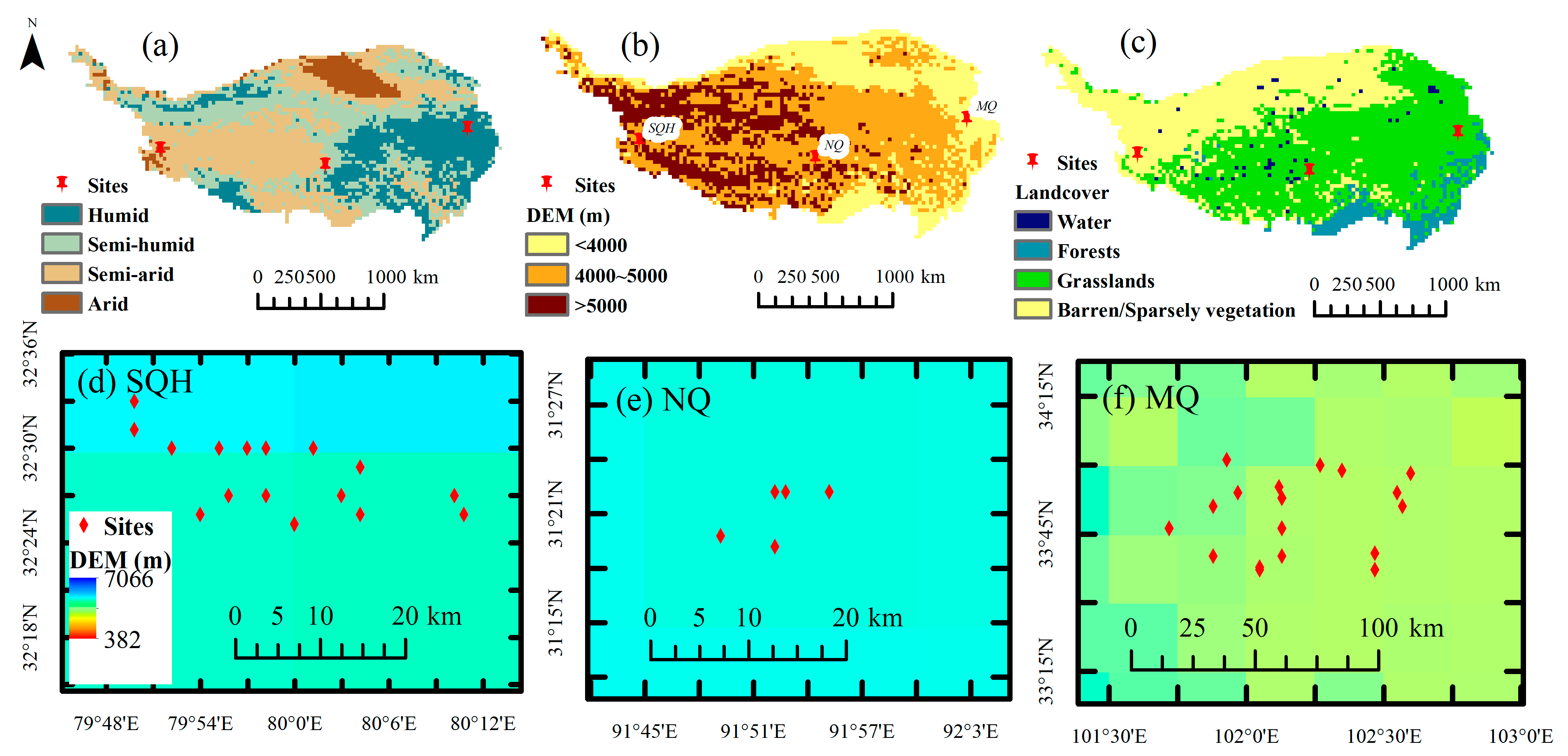
2.1. Study Area

The Qinghai-Tibet Plateau (QTP) is located in southwest China in the range from 73°18′52″ E to 104°46′59″ E and 26°00′12″ N to 39°46′50″ N, which covers the most permafrost in the mid- and low-latitudes. The annual precipitation ranges from 100 to 600 mm, and the maximum air temperature is about 10 ℃ in the summer and almost below 0 ℃ in the other seasons. The climate zonation is based on the aridity index (AI), which can be calculated from precipitation and potential evapotranspiration, as shown in Figure 1a. With an average elevation exceeding 4500 m (Figure 1b), the plateau is surrounded by high mountains. The land covers are forest, grassland, and barren/sparse vegetation from the southeast to the northwest, with grassland accounting for more than half of the QTP (Figure 1c).

2.2. Data

2.2.1. Field Measurement Data

The available in-situ SM monitoring data in the Maqu (MQ), Naqu (NQ), and Shiquanhe (SQH) areas in the growing seasons of June–September in 2014 and 2015 were obtained from the National Tibetan Plateau Data Center. In each area, a varying number of field observation sites were set up to form a network to simultaneously monitor soil temperature and soil moisture. Locations and more details about the three networks are provided in Figure 1 and Table 1.
The MQ, NQ, and SQH monitoring areas are located at the east, central, and southwestern parts of the QTP, covering alpine steppe, typical alpine meadows, and barren land/sparse grassland, respectively [29]. In each area, the observations from the member sites (at site scale) were averaged to match the scale of the CCI-C SM product (at grid scale). At each site, SMC were recorded using soil moisture sensors (ECH2O) at depths of 5, 10, 30, 50, and 80 cm every 15 min. Because microwave signals in the surface layer can only reflect SM of a few centimeters, the SM data for this study was set at 5 cm. The grid daily precipitation, net radiation, relative humidity, and digital elevation model (DEM) data with 0.05° × 0.05° spatial resolution were obtained from the Chinese National Meteorological Centre.

2.2.2. Remote Sensing Data

The CCI-C SM datasets were obtained from the European Space Agency’s (ESA) CCI Soil Moisture website. The datasets of leaf area index (LAI), land surface temperature (LST), and land cover types during 2014 and 2015 were acquired from the MODIS sensors. The SMAP L3 and L4 data with the spatial resolutions of 36 km and 9 km in 2015 from the NASA website were considered as the high accuracy SM product and also used to compare with the results in this work.
There are three types of CCI soil moisture data released by ESA: active product (CCI-A), passive product (CCI-P), and combined product (CCI-C). The CCI products provide daily global surface SMC information at a spatial resolution of 0.25°. The CCI-A products were based on observations from the C-band scatterometers onboard the ERS-1, ERS-2, and MetOp-A and MetOp-B satellites. The CCI-P products utilized passive microwave observations from Nimbus 7 SMMR, DMSP SSM/I, TRMM TMI, Aqua AMSR-E, Coriolis WindSat, GCOM-W1 AMSR2, and SMOS. The CCI-C products were generated by merging all active and passive L2 products. Many previous studies have shown that the CCI-C SM product had higher correlation coefficients and lower errors than the CCI-A or CCI-P products when compared to ground observations [25,30,31]. Thus, the CCI-C SM product was calibrated and validated in this work.

2.3. Models

Figure 2 shows the flowchart of the methodology in this work. Six models were attempted to calibrate the CCI-C SM product, including the simple linear regression model, the logarithmic model, the polynomial model, the logic model, the random forest (RF), and the multiple linear regression (MLR). The first four methods are conventional fitting methods, and they were used to test the linear and nonlinear relationships between the CCI-C and in-situ observations independently of other factors. RF and MLR were used to calibrate the CCI-C SM data using 70% of the in-situ observations from the three networks, while the remaining 30% were used to validate the results. Both RF and MLR were informed by the CCI-C SMC, net radiation (Rn), relative humidity (RH), precipitation, LAI, and LST as inputs.
The best model was determined based on the accuracy assessment. Next, we applied the best model to calibrate the CCI-C product on a zonal basis in recognition of the heterogeneity of surface conditions on the QTP. Different schemes of zonation were tested, namely those based on climate (AI), topography (elevation), and land cover types (Figure 1). We also tried a zonation based on a composite of climate and vegetation (AI + LAI). The climate zones on the QTP include humid, sub-humid, semi-arid, and arid regions based on AI. The established models were applied to the regions that matched the area regarding aridity in which the model was built, i.e., the established model of the MQ area was applied to the humid regions, the model of the NQ area was applied to semi-humid and semi-arid regions, and the model of the SQH area was applied to the arid region. The elevations were divided into three levels (DEM < 4000, 4000 ≤ DEM < 5000, DEM ≥ 5000), and the land covers also were stratified into three types (forest, grass, and barren land or sparse vegetation). The established models were accordingly applied to the matched regions of these levels or types. For the zonation by the AI-LAI composite, which reflects both climate and vegetation characteristics, the regions that the established models were applied to were determined by a similarity approach on a pixel basis, where the similarity is measured by a Euclidean distance between the pixel to be determined and the three networks.

2.4. Accuracy Assessment

Four statistical metrics, including unbiased root mean square error (ubRMSE), Nash-Sutcliffe efficiency coefficient (NSE), Kling–Gupta efficiency (KGE) score, and Pearson correlation coefficient (R), were used to quantitatively evaluate the accuracy of the datasets under study compared to the in-situ observations. The metrics were calculated by the equations listed in Table 2. The ubRMSE measures error without bias, and the larger the ubRMSE, the greater the bias of simulated SMC. The NSE, KGE, and R represent the agreement between the simulation and observations, and the closer to 1, the better the established models performed.

3. Results

3.1. Comparison of CCI-C SM Data with In-Situ Observations

The changes of CCI-C, SMAP L3, and in-situ observed SM during June–September in 2014 and 2015 are shown in Figure 3. The CCI-C SMC was in good agreement in the NQ area, underestimated in the MQ area, and overestimated in the SQH area. Although the SMAP L3 SM performed better than the CCI-C SM, there were a lot of missing data points.
In the MQ area, the precipitation increased significantly from August to September in 2014, resulting in a sharp increase in SMC. The precipitation events were most frequent in 2015, and the SMC in the MQ area was the highest among the three areas. In the NQ area, from June to September 2014, precipitation occurred frequently, and SMC was relatively stable. There was almost no precipitation from 15 July to 30 July in 2015, and the SMC showed the lowest values. From 25 August to 30 September 2015, the precipitation decreased gradually, which caused a decreasing SMC. In the SQH area, there were two typical precipitation events in July and August both in 2014 and 2015, corresponding to the two peaks of SMC. Obviously, precipitation was the main factor affecting SM during the study period.

3.2. Performance of Conventional Fitting Methods

The four fitting methods were used in the three areas to establish the relationship between the in-situ observed and CCI-C SM data (Figure 4). In the MQ area, the linear and logic fitting curves almost coincided, and the logarithmic and polynomial fitting curves were higher when SMC > 0.25 m3/m3 or SMC < 0.15 m3/m3 (Figure 4a). In the NQ area, polynomial and logic fitting curves almost coincided, and linear and logarithmic fitting curves were higher when SMC > 0.25 m3/m3 or SMC < 0.15 m3/m3, but the logarithmic fitting curve was lower when 0.15 < SMC < 0.25 m3/m3 (Figure 4b). In the SQH area, the four fitting curves showed larger differences when SMC > 0.30 m3/m3 or SMC < 0.20 m3/m3 (Figure 4c).
According to the statistical scores, the accuracy of the calibrated CCI-C SM by the four fitting methods was similar in the three areas (Table 3). The highest accuracy was found in the NQ area, and the average values of NSE, KGE, ubRMSE, and R were 0.754, 0.813, 0.028, and 0.868, respectively. They were close to the statistical scores of the in-situ observed and CCI-C SMC, with 0.704, 0.861, 0.028, and 0.870, respectively. However, based on the statistical scores between the in-situ observed and CCI-C SMC in MQ and SQH areas, the four fitting methods significantly improved the CCI-C SMC’s accuracy (Table 3).
In brief, there was no obvious difference among the four fitting methods. The simple linear model could also be a useful method to calibrate the CCI-C SM compared with other methods.

3.3. Calibrated Results Using Machine Learning Method

The daily precipitation, net radiation, relative humidity, LAI, and LST were input as the forcing data of the random forest (RF) and multiply linear regression (MLR) to simulate the SMC in the MQ, NQ, and SQH areas (Figure 5). Since the accuracy of simple linear regression (LR) was similar to that of other statistical methods, we compared the accuracy of this method with that of the random forest and multiple linear regression.
In the MQ area, almost all of the red marks were below the 1:1 line, and the blue marks concentrated around the 1:1 line, indicating that the CCI-C product underestimated SMC and the RF, MLR, and LR improved the accuracy of the CCI-C SMC. The MLR and LR overestimated the SMC when the in-situ observed SM > 0.45 m3/m3 compared with RF. The NSE and KGE of RF were higher than those of MLR and LR, while the ubRMSE and R values had no obvious difference (Figure 6).
In the NQ area, the CCI-C SMC was consistent with the in-situ observed SMC, and both the calibrated and validation data concentrated around the 1:1 line. The simulated SMC between 0.2 and 0.3 m3/m3 by RF were closer to the 1:1 line, but the SMC were underestimated by MLR and LR. According to the statistical scores, the NSE, KGE, and R of RF were higher than those of MLR and LR, and the ubRMSE had no obvious difference (Figure 6).
In the SQH area, the CCI-C product overestimated SMC. In comparison to the statistical scores, the MLR performed better than the RF and LR. The statistical scores of the calibration and validation data had larger differences than those in MQ and SQH. However, the simulated SMC also concentrated around the 1:1 line, and the accuracy of CCI-C SMC was significantly improved.

3.4. Spatial Performance of the Calibrated SM Data in 2015 for Demonstration

The CCI-C SMC was calibrated based on the established models by RF with the three networks in the growing season (June–Sept) of 2015. The mean daily calibrated SMC based on the zonation of DEM, AI, land cover, and composite climate-vegetation (AI + LAI) are shown in Figure 7a–d, respectively.
In Figure 7a, the calibrated SMC based on the DEM zonation on the north of QTP was higher than that based on the AI zonation and land cover zonation. Because the elevation on the north side of QTP was largely lower than 4000 m, the SMC calibrated by the established MQ network was overestimated, especially in the Qaidam basin (referring to Figure 7b–d). In Figure 7b, the high values of the calibrated SMC based on the AI zonation occurred in a small part of the northwest and the majority of the southeast on QTP. The SMC was extremely low in the Qaidam basin and a small portion of the ’TP’s southeast. In Figure 7c, there was barren or sparse vegetation on the northwestern QTP, and thus the SMC calibrated by the models established from the SQH network was lower than that in Figure 7a,b,d. The patterns of Figure 7b,c were similar to those of AI and land cover in Figure 1. Based on the composite of AI and LAI zonation, the SMC was calibrated and shown in Figure 7d. The areas with higher values were reduced from the southeast to the northwest of the QTP.
The SMAP L3 SM performed better than the CCI-C SM, but there were a lot of missing data points on the QTP (Figure 3). The SMAP L4 SM filled the gaps, and the mean daily SMC in June–September 2015 is shown in Figure 8. The high values of SMAP SMC were mainly distributed in the southeastern QTP and declined from the southeast to the northwest of the QTP. Although the values of SMAP SMC were lower than the calibrated CCI-C SMC on the composite of AI and LAI zonation (Figure 7d), the spatial pattern of SMAP SM was similar to Figure 7d. According to the in-situ observed SMC in Figure 3, the SMAP product underestimated SMC in the SQH area. Therefore, the CCI-C SM calibrated based on the composite of AI and LAI zonation is a useful SM dataset on the QTP.

4. Discussion

4.1. Applicability of CCI-C SM Product on the QTP

The CCI-C SM product was found to be able to represent the temporal variations of the SM on the QTP while tending to be larger than the in-situ observations, as observed in all three validation areas. The tendency to overestimate was also observed in previous studies conducted in Spain [32], East Africa [25], North China [28], and Southwest China [26], respectively.
The accuracy of CCI-C SMC was significantly higher in the NQ area than in the other areas. This may be due to the fact that the NQ area is characterized by a land cover type of alpine meadow, which has a relatively low above-ground biomass and little effect on satellite retrieval [33]. In the MQ area, the high above-ground biomass has a greater impact on microwave signals [7,34]. As a result, the CCI-C product underestimated the SM in the MQ area, although it had a higher correlation coefficient with the in-situ measurements. The higher correlation coefficient can probably be explained by the fact that dense vegetation affects the magnitude of SM obtained from microwave signals but not the detection of temporal variations in SM. In arid regions, microwave signals may penetrate deeper into the soil due to soil dryness, resulting in an overestimated SMC [7,35]. The CCI-C product failed to detect the temporal SM changes in the SQH area due to the large amount of unavailable data in this area. It is always a challenge for the CCI missions to acquire SM information in very wet or very dry areas where extensive missing data is present in the data products [19]. In such areas, low signal-to-noise ratios were the main cause of the failure of satellite SM retrievals [36,37]. Furthermore, extreme climatic conditions (dry and cold, covered in snow all year) were to blame for the low satellite signals received [38,39,40,41].
The CCI-C SM product was reported to agree well with field measurements in the Irish and Spanish site networks, while poor results were obtained in Finland [27]. The main reason for low performance in Finland was the long, cold winter and the strong backscattering changes related to the freeze and thaw cycles [42]. Our study concurred with these findings, i.e., the CCI-C SM product performs better in semi-arid areas, but it is not satisfactory to track the temporal dynamics of SM in arid regions.
The active and passive sensors complemented each other under different underlying surface conditions [43,44,45]. Generally, radiometers perform better in dry areas, while scatterometers perform better in areas with dense vegetation [39,42]. The CCI-C product, combining the synergy of the CCI-A and CCI-P microwave products, reduces the errors [20] through a merging algorithm [46]. Many previous studies [21,27,42] found that the CCI-C product performed best at reflecting SM conditions. The assessment of CCI-C on the QTP also well demonstrated the ability of this product in an extremely high-altitude, cold, and climatically complex region. Our study also indicated the CCI-C product biased the magnitude of SMC on the QTP. Previous studies suggested that statistical regression methods can be utilized to remove biases in passive microwave SM data [47]. Our results indicate a random forest method as a promising method to rectify the satellite SM data.

4.2. Temporal and Spatial Changes in SMC on the QTP

Previous studies have shown that the accuracy of remote sensing SM data is highly dependent on underlying surface conditions, soil types [18,48], and climatic conditions [49]. In search of better performance in calibrating SM data, we tested several models, as suggested in the literature, based on different zonation by topography, land cover, vegetation, and climate. Our investigation revealed that SMC peaks in each area were closely associated with typical precipitation events, which is consistent with previous findings that precipitation is the primary factor influencing SM [50]. This is particularly meaningful when the QTP is changing toward a warmer and wetter climate [51]. The calibrated CCI-C product exhibited a typical distribution pattern of SMC on the QTP [15,16,52,53], decreasing from the southeast to the northwest.
The values of the calibrated CCI-C SM data in the humid area were relatively high, while the values in the arid and semi-arid areas were relatively low. Similar spatial distributions of SMC were also reported in previous results [14,17,53,54]. In the arid climate zone, SMC was low throughout the study period. The average SMC on the QTP from June to September 2015 ranged from 0–0.51 m3/m3. Previous reports indicated that the surface SMC is relatively high in the southeastern plateau, relatively low in the middle plateau, and dry in the semi-desert and desert regions of the western plateau [52]. Our results align well with climatic patterns on the QTP, i.e., from the southeast to the northwest, alpine humid regions transition to semi-humid regions, alpine semi-arid regions, and then arid regions [11].
Air temperature, precipitation, and LAI showed similar decreasing spatial distribution patterns toward the northwest as SM. During the growing seasons, changes in SM were mainly affected by precipitation and evaporation [50,55,56]. Therefore, the high SMC in the arid regions of the QTP in July to August, as recorded by our calibrated dataset, was mainly attributed to precipitation events because precipitation can immediately increase SMC in these regions [57]. The higher SMC in the southeast is a combined result of abundant rainfall and the high water-holding capacity of soils due to the prevalent distribution of finer particle soils in this region [3,56]. The northwestern plateau in the arid and semi-arid climatic zones is characterized by barren land and sparse grassland as land cover, low temperatures, and low SMC due to low precipitation [58].

5. Conclusions

Using field observations of SM data, we evaluated the applicability of CCI-C SM products on the QTP. Our results showed that the CCI-C SM data were biased. Several methods were developed to calibrate the CCI-C SM data on a zonal basis based on the spatial discrimination of climatic, topographical, land cover, and vegetation characteristics in the QTP. The results showed that the random forest method performed the best among the methods. The calibrated CCI-C SM data reveal a spatial pattern of soil moisture decreasing from the southeast to the northwest on the QTP, which is consistent with what the SMAP data present. The main factors affecting the SMC from June to September on the QTP include air temperature, precipitation, and land cover types. Our results demonstrate that the random forest method based on composite climate and vegetation zonation can effectively improve the accuracy of CCI-C SM products on the QTP. The calibrated CCI-C SM products can thus serve as an important data basis for land surface studies in data-scarce regions such as the QTP.
However, there are some limitations to the method used in this work. It depended on the spatial zonation method, which affected the results of the random forest method directly. In addition, the spatial zonation was limited by the observed data, which affected the distribution of the calculated SM. In the next work, we hope we can define a more suitable spatial zonation method with more observation data to improve the simulation accuracy.

Author Contributions

Conceptualization, Y.L.; Data curation, G.L.; Writing—original draft, W.Y. All authors have read and agreed to the published version of the manuscript.

Funding

This research was funded by the National Natural Science Foundation of China, grant number 41901076, 41931180, and 41701019.

Data Availability Statement

Not applicable.

Acknowledgments

The authors thank Zhuotong Nan from Nanjing Normal University for improving the language.

Conflicts of Interest

The authors declare no conflict of interest.

References

  1. Dickinson, R.E. Land surface processes and climate—Surface albedos and energy balance. Adv. Geophys. 1983, 25, 305–353. [Google Scholar]
  2. Li, R.; Zhao, L.; Wu, T.; Ding, Y.; Xiao, Y.; Hu, G.; Zou, D.; Li, W.; Yu, W.; Jiao, Y.; et al. The impact of surface energy exchange on the thawing process of active layer over the northern Qinghai–Xizang Plateau, China. Environ. Earth Sci. 2014, 72, 2091–2099. [Google Scholar] [CrossRef]
  3. Li, H.; Shen, W.; Zou, C.; Jiang, J.; Fu, L.; She, G. Spatio-temporal variability of soil moisture and its effect on vegetation in a desertified aeolian riparian ecotone on the Tibetan Plateau, China. J. Hydrol. 2013, 479, 215–225. [Google Scholar]
  4. Zucco, G.; Brocca, L.; Moramarco, T.; Morbidelli, R. Influence of land use on soil moisture spatial–temporal variability and monitoring. J. Hydrol. 2014, 516, 193–199. [Google Scholar] [CrossRef]
  5. Stamenkovic, J.; Guerriero, L.; Ferrazzoli, P.; Notarnicola, C.; Greifeneder, F.; Thiran, J.P. Soil moisture estimation by SAR in Alpine fields using Gaussian process regressor trained by model simulations. IEEE. Geosci. Remote Sens. 2017, 55, 4899–4912. [Google Scholar] [CrossRef]
  6. Lee, J.H.; Cosh, M.; Starks, P.; Toth, Z. Self-Correction of Soil Moisture Ocean Salinity (SMOS) Soil Moisture Dry Bias. Can. J. Remote Sens. 2019, 45, 814–828. [Google Scholar]
  7. Ma, C.F.; Li, X.; Wei, L.; Wang, W.Z. Multi-scale validation of SMAP soil moisture products over cold and arid regions in northwestern China using distributed ground observation data. Remote Sens. 2017, 9, 327. [Google Scholar] [CrossRef]
  8. Qin, D.; Ding, Y.; Xiao, C.; Kang, S.; Ren, J.; Yang, J.; Zhang, S. Cryospheric Science: Research framework and disciplinary system. Natl. Sci. Rev. 2018, 5, 255–268. [Google Scholar]
  9. Yang, M.; Nelson, F.E.; Shiklomanov, N.I.; Guo, D.; Wan, G. Permafrost degradation and its environmental effects on the Tibetan Plateau: A review of recent research. Earth Sci. Rev. 2010, 103, 31–44. [Google Scholar] [CrossRef]
  10. Ma, Y.; Su, Z.; Koike, T.; Yao, T.; Ishikawa, H.; Ueno, K.; Menenti, M. On measuring and remote sensing surface energy partitioning over the Tibetan Plateau––from GAME/Tibet to CAMP/Tibet. Phys. Chem. Earth. 2003, 28, 63–74. [Google Scholar] [CrossRef]
  11. Yang, K.; Ye, B.; Zhou, D.; Wu, B.; Foken, T.; Qin, J.; Zhou, Z. Response of hydrological cycle to recent climate changes in the Tibetan Plateau. Clim. Chang. 2011, 109, 517–534. [Google Scholar] [CrossRef]
  12. Li, C.; Sun, H.; Wu, X.; Han, H. An approach for improving soil water content for modeling net primary production on the Qinghai-Tibetan Plateau using Biome-BGC model. Catena 2020, 184, 104253. [Google Scholar] [CrossRef]
  13. Yang, J.; Ma, Y.M. Soil temperature and moisture features of typical underlying surface in the Tibet Plateau. J. Glaciol. Geocryol. 2012, 34, 813–820. [Google Scholar]
  14. Liu, Q.; Du, J.; Shi, J.; Jiang, L. Analysis of spatial distribution and multi-year trend of the remotely sensed soil moisture on the Tibetan Plateau. Sci. China Earth Sci. 2013, 56, 2173–2185. [Google Scholar]
  15. Zeng, J.; Li, Z.; Chen, Q.; Bi, H.; Qiu, J.; Zou, P. Evaluation of remotely sensed and reanalysis soil moisture products over the Tibetan Plateau using in-situ observations. Remote Sens. Environ. 2015, 163, 91–110. [Google Scholar]
  16. Xi, J.J.; Tian, H.; Zhang, T. Applicability evaluation of AMSR-E remote sensing soil moisture products in Qinghai-Tibet plateau. Trans. CSAE 2014, 30, 194–202. [Google Scholar]
  17. Wan, H.; Gao, P.; Guo, P. Applicability evaluation of FY—3B remote sensing soil moisture products in the Tibetan plateau. J. Arid Land Res. Environ. 2017, 32, 132–137. [Google Scholar]
  18. Mohanty, B.P.; Cosh, M.H.; Lakshmi, V.; Montzka, C. Soil moisture remote sensing: State-of-the-Science. Vadose Zone J. 2017, 16, 1–9. [Google Scholar]
  19. Dorigo, W.; Wagner, W.; Albergel, C.; Albrecht, F.; Balsamo, G.; Brocca, L.; Chung, D.; Ertl, M.; Forkel, M.; Gruber, A.; et al. ESA CCI Soil Moisture for improved Earth system understanding: State-of-the art and future directions. Remote Sens. Environ. 2017, 203, 185–215. [Google Scholar]
  20. Liu, Y.Y.; Parinussa, R.M.; Dorigo, W.A.; De Jeu, R.A.M.; Wagner, W.; van Dijk, A.I.J.M.; McCabe, M.F.; Evans, J.P. Developing an improved soil moisture dataset by blending passive and active microwave satellite-based retrievals. Hydrol. Earth Syst. Sci. 2011, 15, 425–436. [Google Scholar]
  21. Liu, Y.Y.; Dorigo, W.A.; Parinussa, R.M.; de Jeu, R.A.M.; Wagner, W.; McCabe, M.F.; Evans, J.P.; van Dijk, A.I.J.M. Trend-preserving blending of passive and active microwave soil moisture retrievals. Remote Sens. Environ. 2012, 123, 280–297. [Google Scholar] [CrossRef]
  22. Wagner, W.; Dorigo, W.; de Jeu, R.; Fernandez, D.; Benveniste, J.; Haas, E.; Ertl, M. Fusion of active and passive microwave observations to create an essential climate variable data record on soil moisture. ISPRS Ann. 2012, 7, 315–321. [Google Scholar] [CrossRef]
  23. Dorigo, W.A.; de Jeu, R.A.M.; Chung, D.; Parinussa, R.M.; Liu, Y.; Wagner, W.; Fernandez-Prieto, D. Evaluating global trends (1988–2010) in harmonized multi-satellite surface soil moisture. Geophys. Res. Lett. 2012, 39, L18405. [Google Scholar]
  24. Albergel, C.; de Rosnay, P.; Balsamo, G.; Isaksen, L.; Muñoz-Sabater, J. Soil moisture analyses at ECMWF: Evaluation using global ground-based in situ observations. J. Hydrometeorol. 2012, 13, 1442–1460. [Google Scholar]
  25. McNally, A.; Shukla, S.; Arsenault, K.; Wang, S.; Peters-Lidard, C.; Verdin, J. Evaluating ESA CCI soil moisture in East Africa. Int. J. Appl. Earth Obs. Geoinf. 2016, 48, 96–109. [Google Scholar] [PubMed]
  26. Peng, J.; Niesel, J.; Loew, A.; Zhang, S.Q.; Wang, J. Evaluation of satellite and reanalysis soil moisture products over southwest china using ground-based measurements. Remote Sens. 2015, 7, 15729–15747. [Google Scholar] [CrossRef]
  27. Pratola, C.; Barrett, B.; Gruber, A.; Dwyer, E. Quality assessment of the CCI ECV soil moisture product using ENVISAT ASAR wide swath data over Spain, Ireland and Finland. Remote Sens. 2015, 7, 15388–15423. [Google Scholar]
  28. Wang, S.; Mo, X.; Liu, S.; Lin, Z.; Hu, S. Validation and trend analysis of ECV soil moisture data on cropland in North China Plain during 1981–2010. Int. J. Appl. Earth Obs. 2016, 48, 110–121. [Google Scholar] [CrossRef]
  29. Wang, Z.; Wang, Q.; Zhao, L.; Wu, X.; Yue, G.-Y.; Zou, D.-F.; Nan, Z.-T.; Liu, G.-Y.; Pang, Q.-Q.; Fang, H.-B.; et al. Mapping the vegetation distribution of the permafrost zone on the Qinghai-Tibet Plateau. J. MT Sci. Engl. 2016, 13, 1035–1046. [Google Scholar]
  30. Holmes, T.R.H.; De Jeu, R.A.M.; Owe, M.; Dolman, A.J. Land surface temperature from Ka band (37 GHz) passive microwave observations. J. Geophys. Res. Atmos. 2009, 114, D04113. [Google Scholar]
  31. Fang, L.; Hain, C.R.; Zhan, X.; Anderson, M.C. An inter-comparison of soil moisture data products from satellite remote sensing and a land surface model. Int. J. Appl. Earth Obs. 2016, 48, 37–50. [Google Scholar]
  32. Rahman, K.U.; Shang, S. A Regional Blended Precipitation Dataset over Pakistan Based on Regional Selection of Blending Satellite Precipitation Datasets and the Dynamic Weighted Average Least Squares Algorithm. Remote Sens. 2020, 12, 4009. [Google Scholar] [CrossRef]
  33. González-Zamora, Á.; Sánchez, N.; Pablos, M.; Martínez-Fernández, J. CCI soil moisture assessment with SMOS soil moisture and in situ data under different environmental conditions and spatial scales in Spain. Remote Sens. Environ. 2018, 225, 469–482. [Google Scholar]
  34. Zhang, Z.J.; Sun, G.Q. Model investigation of the effect of vegetation on passive microwave soil moisture retrieval. Microwave Remote Sensing of the Atmosphere and Environment III. In Proceedings of the Third International Asia-Pacific Environmental Remote Sensing Remote Sensing of the Atmosphere, Ocean, Environment, and Space, Hangzhou, China, April 2003; Volume 4894, pp. 140–150. [Google Scholar] [CrossRef]
  35. Parinussa, R.M.; Holmes, T.R.H.; de Jeu, R.A.M. Soil moisture retrievals from the WindSat spaceborne polarimetric microwave radiometer. IEEE. Geosci. Remote Sens. 2012, 50, 2683–2694. [Google Scholar] [CrossRef]
  36. Shi, J.; Jiang, L.; Zhang, L.; Chen, K.S.; Wigneron, J.P.; Chanzy, A.; Jackson, T.J. Physically based estimation of bare-surface soil moisture with the passive radiometers. IEEE. Geosci. Remote Sens. 2006, 44, 3145–3153. [Google Scholar] [CrossRef]
  37. van der Schrier, G.; Barichivich, J.; Briffa, K.R.; Jones, P.D. A scPDSI-based global data set of dry and wet spells for 1901–2009. J. Geophys. Res. Atmos. 2013, 118, 4025–4048. [Google Scholar] [CrossRef]
  38. Gruber, A.; Su, C.-H.; Crow, W.T.; Zwieback, S.; Dorigo, W.A.; Wagner, W. Estimating error cross-correlations in soil moisture data sets using extended collocation analysis. J. Geophys. Res. Atmos. 2016, 121, 1208–1219. [Google Scholar] [CrossRef]
  39. Barichivich, J.; Briffa, K.R.; Myneni, R.; Schrier, G.V.d.; Dorigo, W.; Tucker, C.J.; Osborn, T.J.; Melvin, T.M. Temperature and Snow-Mediated Moisture Controls of Summer Photosynthetic Activity in Northern Terrestrial Ecosystems between 1982 and 2011. Remote Sens. 2014, 6, 1390–1431. [Google Scholar] [CrossRef]
  40. Cosh, M.H.; Ochsner, T.; McKee, L.; Dong, J.; Basara, J.B.; Evett, S.R.; Hatch, C.E.; Small, E.E.; Steele-Dunne, S.C.; Zreda, M.; et al. The soil moisture active passive Marena, Oklahoma, in situ sensor testbed (SMAP-MOISST): Testbed design and evaluation of in situ sensors. Vadose Zone J. 2016, 15, vzj2015.09.0122. [Google Scholar]
  41. Dorigo, W.A.; Wagner, W.; Hohensinn, R.; Hahn, S.; Paulik, C.; Xaver, A.; Gruber, A.; Drusch, M.; Mecklenburg, S.; van Oevelen, P.; et al. The International Soil Moisture Network: A data hosting facility for global in situ soil moisture measurements. Hydrol. Earth Syst. Sci. 2011, 15, 1675–1698. [Google Scholar]
  42. Loew, A.; Stacke, T.; Dorigo, W.; de Jeu, R.; Hagemann, S. Potential and limitations of multidecadal satellite soil moisture observations for selected climate model evaluation studies. Hydrol. Earth Syst. Sci. 2013, 17, 3523–3542. [Google Scholar]
  43. Dorigo, W.A.; Gruber, A.; De Jeu, R.A.M.; Wagner, W.; Stacke, T.; Loew, A.; Albergel, C.; Brocca, L.; Chung, D.; Parinussa, R.M.; et al. Evaluation of the ESA CCI soil moisture product using ground-based observations. Remote Sens. Environ. 2015, 162, 380–395. [Google Scholar] [CrossRef]
  44. Albergel, C.; de Rosnay, P.; Gruhier, C.; Muñoz-Sabater, J.; Hasenauer, S.; Isaksen, L.; Kerr, Y.; Wagner, W. Evaluation of remotely sensed and modelled soil moisture products using global ground-based in situ observations. Remote Sens. Environ. 2012, 118, 215–226. [Google Scholar]
  45. Dorigo, W.A.; Scipal, K.; Parinussa, R.M.; Liu, Y.Y.; Wagner, W.; de Jeu, R.A.M.; Naeimi, V. Error characterisation of global active and passive microwave soil moisture datasets. Hydrol. Earth Syst. Sci. 2010, 14, 2605–2616. [Google Scholar]
  46. Taylor, C.M.; de Jeu, R.A.; Guichard, F.; Harris, P.P.; Dorigo, W.A. Afternoon rain more likely over drier soils. Nature 2012, 489, 423–426. [Google Scholar] [CrossRef] [PubMed]
  47. Gruber, A.; Dorigo, W.A.; Crow, W.; Wagner, W. Triple collocation-based merging of satellite soil moisture retrievals. IEEE. Geosci. Remote Sens. 2017, 55, 6780–6792. [Google Scholar] [CrossRef]
  48. Al-Yaari, A.; Wigneron, J.P.; Kerr, Y.; de Jeu, R.; Rodriguez-Fernandez, N.; Van Der Schalie, R.; Bitar, A.A.; Mialon, A.; Richaume, P.; Dolman, A.; et al. Testing regression equations to derive long-term global soil moisture datasets from passive microwave observations. Remote Sens. Environ. 2016, 180, 453–464. [Google Scholar]
  49. Elnaggar, A.A.; Noller, J.S. Application of remote-sensing data and decision-tree analysis to mapping salt-affected soils over large areas. Remote Sens. 2010, 2, 151–165. [Google Scholar] [CrossRef]
  50. Wu, X.; Fang, H.; Zhao, Y.; Smoak, J.; Li, W.; Shi, W.; Sheng, Y.; Zhao, L.; Ding, Y. A conceptual model of the controlling factors of soil organic carbon and nitrogen densities in a permafrost-affected region on the eastern Qinghai-Tibetan Plateau. J. Geophys. Res. Biogeosci. 2017, 122, 1705–1717. [Google Scholar]
  51. Findell, K.L.; Eltahir, E.A.B. An analysis of the soil moisture-rainfall feedback, based on direct observations from Illinois. Water Resour. Res. 1997, 33, 725–735. [Google Scholar] [CrossRef]
  52. Zhang, G.; Nan, Z.; Zhao, L.; Liang, Y.; Cheng, G. Qinghai-Tibet Plateau wetting reduces permafrost thermal responses to climate warming. Earth Planet. Sci. Lett. 2021, 562, 116858. [Google Scholar] [CrossRef]
  53. Su, Z.; Wen, J.; Dente, L.; van der Velde, R.; Wang, L.; Ma, Y.; Yang, K.; Hu, Z. The Tibetan Plateau observatory of plateau scale soil moisture and soil temperature (Tibet-Obs) for quantifying uncertainties in coarse resolution satellite and model products. Hydrol. Earth Syst. Sci. 2011, 15, 2303–2316. [Google Scholar] [CrossRef]
  54. Shi, L.; Du, J.; Zhou, K.S.; Zhuo, G. Temporal and spatial evolution of soil moisture over the Tibetan Plateau from 1980 to 2012. J. Glaciol. Geocryol. 2016, 38, 1241–1248. [Google Scholar]
  55. Méndez-Barroso, L.A.; Vivoni, E.R.; Watts, C.J.; Rodríguez, J.C. Seasonal and interannual relations between precipitation, surface soil moisture and vegetation dynamics in the North American monsoon region. J. Hydrol. 2009, 377, 59–70. [Google Scholar] [CrossRef]
  56. Yang, M.X.; Yao, T.D.; He, Y.Q. The role of soil moisture-energy distribution and melting-freezing processes on seasonal shift in Tibetan Plateau. J. MT Sci. Engl. 2002, 20, 536–558. [Google Scholar]
  57. Qi, W.; Zhang, B.; Pang, Y.; Zhao, F.; Zhang, S. TRMM-Data-Based Spatial and Seasonal Patterns of Precipitation in the Qinghai-Tibet Plateau. Sci. Geogr. Sin. 2013, 33, 999–1005. [Google Scholar]
  58. Wu, X.; Zhao, L.; Wu, T.; Chen, J.; Pang, Q.; Du, E.; Fang, H.; Wang, Z.; Zhao, Y.; Ding, Y. Observation of CO2 degassing in Tianshuihai Lake Basin of the Qinghai-Tibetan Plateau. Environ. Earth Sci. 2013, 68, 865–870. [Google Scholar] [CrossRef]
Figure 1. Zonation by climate (a), elevation (b), and land cover type (c), and the soil moisture (SM) observation networks in the SQH (d), NQ (e), and MQ (f) areas on the Qinghai-Tibet Plateau (QTP), composed of SM sites marked in red diamonds. The locations of the networks are shown in (b).
Remotesensing 15 00918 g001
Figure 2. The flowchart of methology.
Remotesensing 15 00918 g002
Figure 3. SMC time series from two satellite-based CCI-C and SMAP products and in-situ observations in the MQ (a,b), NQ (c,d), and SQH (e,f) areas from June–September in 2014 and 2015, respectively.
Remotesensing 15 00918 g003
Figure 4. Scatter plots and fitting curves of the in-situ observed and CCI-C SM data (m3/m3) in the MQ, NQ, and SQH areas during June to September in 2014 and 2015. Four fitting methods were used to fit the data.
Remotesensing 15 00918 g004
Figure 5. Contrast of the CCI-C SM data (red mark) versus the simulations (blue mark) by the fit models against the in-situ observed SMC data in the MQ, NQ, and SQH areas. RF: random forest; MLR: multiple linear regression; LR: simple linear regression. The diagonal lines represent a 1:1 line. Squares and dots represent the calibration data (70% of the total) and validation data (the remaining 30%), respectively. SM-obs: in-situ SM data; SM-sim/CCI: the data from model fits or the CCI-C dataset.
Remotesensing 15 00918 g005
Figure 6. Heat map of statistical scores, including the Nash-Sutcliffe efficiency coefficient (NSE), Kling–Gupta efficiency (KGE), unbiased root mean square error (ubRMSE), and correlation coefficient (R), based on the fits by RF, MLR, and LR in MQ, NQ, and SQH. The subscripts c and v indicate the calibration and validation data sets, respectively.
Remotesensing 15 00918 g006
Figure 7. Spatial distributions of the caliburated CCI-C SM data (m3/m3) based on zonation by topography (a), climate (b), land cover type (c), and composite climate-vegetation (d).
Remotesensing 15 00918 g007
Figure 8. Mean daily SMC from the NASA’s Soil Moisture Active Passive (SMAP) instrument during June–September in 2015 as a reference.
Remotesensing 15 00918 g008
Table 1. Descriptions of the SM observation sites forming the three networks of NQ, MQ, and SQH on the QTP.
NetworkSiteLatitude (N)/Longitude (E)Elevation (m)TopographyLand Cover
Naqu
(NQ)
Naqu31°22′/91°53′4509Flat groundGrassland
West31°20′/91°49′4506Flat groundGrassland
South31°19′/91°52′4510Mountain slopeWet meadow
North31°22′/91°52′4507RiverbankGrassland
East31°22′/91°55′4527Flat hill topGrassland
Maqu (MQ)CST_0133°53′/102°08′3431River valleyGrassland
CST_0233°40′/102°08′3449River valleyGrassland
CST_0333°54′/101°58′3507Hill valleyGrassland
CST_0433°46′/101°43′3504Hill valleyGrassland
CST_0533°40′/101°53′3542Hill valleyGrassland
NST_0133°53′/102°08′3431River valleyGrassland
NST_0233°53′/102°08′3434River valleyGrassland
NST_0333°46′/102°08′3513Hill slopeGrassland
NST_0433°37′/102°03′3448River valleyWet meadow
NST_0533°38′/102°03′3476River valleyGrassland
NST_0634°00′/102°16′3428River valleyGrassland
NST_0733°59′/102°21′3430River valleyGrassland
NST_0833°58′/102°36′3473Mountain valleyGrassland
NST_0933°54′/102°33′3434River valleyGrassland
NST_1033°51′/102°34′3512Hill slopeGrassland
NST_1133°41′/102°28′3442River valleyWet meadow
NST_1233°37′/102°28′3441River valleyGrassland
NST_1334°01′/101°56′3519Mountain valleyGrassland
NST_1433°55′/102°07′3432River valleyGrassland
NST_1533°51′/101°53′3752Hill slopeGrassland
Shiquanhe (SQH)SQ0132°29′/80°04′4306Flat groundDesert
SQ0232°30′/80°01′4304Gentle slopeDesert
SQ0332°30′/79°58′4278Gentle slopeDesert
SQ0432°30′/79°57′4269Flat groundSparse grass
SQ0532°30′/79°55′4261Flat groundSparse grass
SQ0632°30′/79°52′4257Flat groundSparse grass
SQ0732°31′/79°50′4280Flat groundDesert
SQ0832°33′/79°50′4306Flat groundDesert
SQ0932°27′/80°03′4275Flat groundDesert
SQ1032°25′/80°00′4275Flat groundGrassland
SQ1132°27′/79°58′4274Flat groundGrassland
SQ1232°27′/79°56′4264Edge of riverbedDesert
SQ1332°26′/79°54′4295Valley bottomDesert
SQ1432°27′/80°10′4368Mountain slopeDesert
SQ1532°26′/80°11′4387Flat groundShrubs
SQ1632°26′/80°04′4288Flat groundDesert
Table 2. Statistical metrics to assess the accuracy of SM data. θ o b s , i and θ C C I , i denote the in-situ observed and CCI-C SM contents (SMC) in the i day, respectively; θ o b s ¯ and θ C C I ¯ denote the average value of the observed and CCI-C SMC, respectively; n is the size of records (Rahman and Shang, 2020).
MetricEquation
NSE
N S E = 1 i = 1 n ( θ o b s , i θ C C I , i ) 2 i = 1 n ( θ o b s , i θ o b s ¯ ) 2
KGE
KGE = 1 ( 1 R ) 2 + ( 1 β ) 2 + ( 1 γ ) 2
β = θ C C I ¯ θ o b s ¯
γ = 1 N I = 1 N ( θ C C I , i θ C C I ¯ ) / θ C C I ¯ / 1 N I = 1 N ( θ o b s , i θ o b s ¯ ) / θ o b s ¯
ubRMSE
ubRMSE = | 1 n i = 1 n ( θ C C I , i θ o b s , i ) 2 ( 1 n i = 1 n ( θ C C I , i θ o b s , i ) ) 2 |
R
R = 1 n i = 1 n [ ( θ C C I , i θ C C I ¯ ) ( θ o b s , i θ o b s ¯ ) ] i = 1 n ( θ C C I , i θ C C I ¯ ) 2 i = 1 n ( θ o b s , i θ o b s ¯ ) 2
Table 3. Statistical scores of four conventional fitting methods measured between the in-situ observed and the calibrated CCI-C SMC data in the three network areas; the underlined values were calculated from the in-situ observed and the CCI-C SM data prior to calibration.
SitesMethodNSEKGEubRMSER
MQCCI−2.349 0.412 0.047 0.742
Linear fit0.551 0.636 0.049 0.742
Logarithmic fit 0.566 0.650 0.048 0.752
Polynomial fit0.569 0.653 0.048 0.754
Logic fit0.539 0.631 0.049 0.734
NQCCI0.704 0.861 0.028 0.870
Linear fit0.758 0.817 0.027 0.870
Logarithmic fit 0.729 0.793 0.029 0.854
Polynomial fit0.764 0.822 0.027 0.874
Logic fit0.764 0.821 0.027 0.874
SQHCCI−9.259 −0.187 0.091 0.774
Linear fit0.599 0.680 0.024 0.774
Logarithmic fit 0.577 0.660 0.025 0.760
Polynomial fit0.601 0.682 0.024 0.775
Logic fit0.593 0.684 0.024 0.770
Disclaimer/Publisher’s Note: The statements, opinions and data contained in all publications are solely those of the individual author(s) and contributor(s) and not of MDPI and/or the editor(s). MDPI and/or the editor(s) disclaim responsibility for any injury to people or property resulting from any ideas, methods, instructions or products referred to in the content.

