Abstract
Slope failures, subsidence, earthworks, consolidation of waste dumps, and erosion are typical active deformation processes that pose a significant hazard in current and abandoned mining areas, given their considerable potential to produce damage and affect the population at large. This work proves the potential of exploiting space-borne InSAR and airborne LiDAR techniques, combined with data inferred through a simple slope stability geotechnical model, to obtain and update inventory maps of active deformations in mining areas. The proposed approach is illustrated by analyzing the region of Sierra de Cartagena-La Union (Murcia), a mountainous mining area in southeast Spain. Firstly, we processed Sentinel-1 InSAR imagery acquired both in ascending and descending orbits covering the period from October 2016 to November 2021. The obtained ascending and descending deformation velocities were then separately post-processed to semi-automatically generate two active deformation areas (ADA) maps by using ADATool. Subsequently, the PS-InSAR LOS displacements of the ascending and descending tracks were decomposed into vertical and east-west components. Complementarily, open-access, and non-customized LiDAR point clouds were used to analyze surface changes and movements. Furthermore, a slope stability safety factor (SF) map was obtained over the study area adopting a simple infinite slope stability model. Finally, the InSAR-derived maps, the LiDAR-derived map, and the SF map were integrated to update a previously published landslides’ inventory map and to perform a preliminary classification of the different active deformation areas with the support of optical images and a geological map. Complementarily, a level of activity index is defined to state the reliability of the detected ADA. A total of 28, 19, 5, and 12 ADAs were identified through ascending, descending, horizontal, and vertical InSAR datasets, respectively, and 58 ADAs from the LiDAR change detection map. The subsequent preliminary classification of the ADA enabled the identification of eight areas of consolidation of waste dumps, 11 zones in which earthworks were performed, three areas affected by erosion processes, 17 landslides, two mining subsidence zone, seven areas affected by compound processes, and 23 possible false positive ADAs. The results highlight the effectiveness of these two remote sensing techniques (i.e., InSAR and LiDAR) in conjunction with simple geotechnical models and with the support of orthophotos and geological information to update inventory maps of active deformation areas in mining zones.
1. Introduction
Mining areas are usually affected by active deformations caused by subsidence and slope instabilities phenomena, as well as other processes such as erosion and consolidation of mining waste dumps, which may appear both during operation and after closure. Mining earthmoving operations (i.e., excavations and waste dumps) also alter the topography of the ground surface.
Ground movements in mining areas are usually monitored using surface (e.g., leveling) and subsurface techniques (e.g., surveying, settlement cells, or inclinometers), which require in situ measurements and represent a costly solution [1]. Optical remote sensing has the ability to detect and map some ADAs based on their geomorphological features (e.g., tension cracks), although it is highly susceptible to external factors such as the subjective opinion of experts and their expertise, and very time-consuming [2]. Interferometric Synthetic Aperture Radar (InSAR) is a technique that has been proven very effective for the detection, the delineation of boundaries, and the assessment of ADAs [3,4,5]. InSAR can provide displacement time series estimations up to submillimeter accuracy [6]. However, the interferometric quality is often affected by the inherent presence of temporal decorrelation when the SAR images are collected in the repeat-pass mode, which leads to interferometric coherence loss, especially in forested and anthropogenically modified areas.
In contrast, multi-temporal LiDAR (Light Detection and Ranging) datasets used to produce an inventory map are not only conducive to a loss of resolution but also allow a better capture of subtle changes on quick deformation [7,8,9]. In fact, previous studies have demonstrated the capability of differential LiDAR to measure changes caused by earthquakes [10,11,12], coastal processes [13,14], mining subsidence [12], and landslides [7,12,15], among other events [9]. LiDAR enables us to obtain of high-quality three-dimensional terrain data in terms of density and accuracy [16]. Typically, the accuracy of LiDAR can reach a very few centimeters of root-mean-square error and a pulse density of 0.5–1 pulses per square meter [16,17,18]. Similar to LiDAR, unmanned aerial vehicle (UAV) photogrammetry enables monitoring ground displacements based on the high-resolution differential DEMs (digital elevation models) [19,20,21].
Consequently, to improve the ability to detect and update the active deformation inventory maps, the application of LiDAR has been adopted as a complementary technique for the updating of active areas in this work. Consequently, the complementarities between both techniques enable to increase the capability to automatically map changes on the ground surface. In the case of landslides, the phenomenon is controlled by geotechnical processes. Then, the addition of external information derived from the implementation of slope stability models permits the identification of the areas prone to landslides (i.e., the areas exhibiting a safety factor lower than one) and thus contributes to the improvement of the identification of potentially unstable slopes. Finally, the use of geological maps and the expert analysis of orthophotos enables the identification of geomorphological features and landforms for the preliminary classification of the ADAs.
The Sierra de Cartagena-La Union (Murcia) has been intensively exploited since the Roman period. From the 19th century up to 1991, the area was intensively exploited using both underground and open-pit mining. Currently, the mining activity has ceased, although multiple deformational processes remain active, constituting a threat to the closest urban areas and becoming an important drawback for the economic and environmental recuperation of this mining area [4].
Previous studies have addressed some issues related to the study of active deformation areas (ADAs), such as stability analyses of abandoned open pit mines and waste dumps [22], ground movements mapping [23], and mining subsidence analysis [24,25,26,27,28,29] in specific areas of the Sierra de Cartagena-La Union. Thus, this work not only updates the existing ADA datasets for the whole Sierra de Cartagena-La Union but also proposes a comprehensive systematic methodology for the automatic mapping and preliminary classification of the ADAs affecting the region.
Therefore, the aim of this paper is to propose a methodology to exploit synergies of LiDAR and InSAR remote sensing techniques to detect active deformation areas in mining areas. This information, jointly with the external geotechnical stability model, the geological map, and the support of orthophotos used to identify geomorphological features, will enable us to update existing inventory maps and to perform a preliminary classification of the phenomena over wide areas. It should be highlighted that the proposed method not only enables the identification of landslides but also the mapping and preliminary classification of other phenomena which usually develop in mining areas, such as consolidation of waste dumps, earthworks, subsidence, and erosion.
The paper is organized as follows. Section 2 provides a general overview of the Sierra Minera and a summary of the datasets used in this study. Section 3 includes a detailed explanation of the proposed methodology. Section 4 shows the main results. Section 5 discusses in detail the obtained results, the classification of the ADAs, and the differences between both technologies for the detection and classification of ADAs. Finally, Section 6 provides the most relevant conclusions of this work.
2. Study Area and Datasets
2.1. Study Area
The Sierra de Cartagena-La Union (Murcia) belongs to the Internal Zones of the Betic Cordillera, in the convergence margin between the African and the Iberian plates, in the south-eastern part of Spain, which is a coastal mountain region [22] (Figure 1).
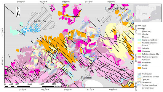
Figure 1.
Geological map of the study area adapted from [22].
The geology of the study area is composed of three tectonically superimposed complex nappes, which are from bottom to top the Nevado-Filábride, the Alpujárride, and the Maláguide complexes. The Nevado-Filábride complex is mainly comprised of Paleozoic to Permo-Triassic marbles, schists, mica schists, and quartzites. The Alpujárride complex is mostly represented by Permian quartzites and phyllites and by a carbonate series of Triassic age containing igneous intrusions [30]. Following, the Maláguide complex, which constitutes the topmost tectonic complex, is composed of Neogene sedimentary rocks (e.g., limestone, sandstone, silt, and conglomerate) [31]. These geological units are covered by thin, loose alluvial Quaternary deposits of gravel, clay, silt, and sand. Figure 1 summarizes the geological units of the study area.
The geological and structural complexity of the region leads to a complex hydrological relation between the different units. Although most of the geological units are not permeable, the Alpujárride marbles, the detritic Miocene rocks, and the Quaternary formations (sand, silt, and clays) are permeable. Yet the permeability values of these units are low according to pumping tests developed by the Spanish Geological and Mining Institute (IGME) in some good points [25].
The Pb and Zn ore deposits, which are associated with the mantle and seam structural setting of the region, have been exploited from the Iberian period [32] and were intensively mined from 1940 to 1990 [29]. This was first carried out by underground mining using the room-and-pillar method. Later, starting in the 1960s, several open-pit mines were developed. Finally, the mining activity in the region ceased in 1991. Currently, there exist some landfills for inert waste in the area.
2.2. Datasets
An original landslide inventory map and a geological map, including the mining facilities (e.g., open pit mines and waste dumps), obtained through photo interpretation and fieldwork, were provided by IGME [23,33] (Figure 1). It should be noted that the landslide inventory map was first elaborated in 1996 and updated in 2010 with the aid of InSAR data and fieldwork [25].
The geo-mechanical properties (i.e., density, friction angle, and cohesion) of the dominant lithologies used for the slope stability analysis presented herein were derived from the work published by López-Vinielles et al. [22]. These values were, in turn, derived from laboratory tests performed by IGME [33].
Elevation normally relates to the potential energy of a slope, being the slope angle a key factor for stability. To determine the dip angle of a slope, the most common strategy is to use a digital terrain model (DTM). In this work, the slope angle values used for the stability analysis performed were derived from a freely available DTM with 5 m grid spacing from the National Geographical Institute of Spain (IGN) [34].
Additionally, two open-access non-specifically acquired, and non-customized LiDAR point cloud datasets covering the study area were downloaded from the online Geoportal of the National Plan for Aerial Orthophotography (PNOA) of Spain [35]. As shown in Table 1, the point clouds were captured with a density of 0.5 points/m2 and automatically classified and colored by RGB (red, green, and blue) obtained from orthophotos of the PNOA with a pixel size of 25 or 50 cm [36].

Table 1.
Basic parameters of the LiDAR datasets from La Unión used in this study [37,38].
Finally, two stacks of descending and ascending Sentinel-1 Single Look Complex (SLC) SAR images were utilized to generate ground deformation maps using InSAR along the line of sight (LOS). A total of 131 Sentinel-1 images in ascending orbit (track No. 103) and 131 in descending orbit (track No. 8) spanning the time interval from 7 October 2016 to 10 November 2021 were processed. A digital surfaces model (DSM) with a 5 m grid spacing from the National Geographical Institute of Spain (IGN) [34] was also employed for the standard Differential- InSAR (D-InSAR) processing.
3. Methodology
This paper introduces a straightforward methodology based on the joint exploitation of InSAR and LiDAR datasets to update inventory maps of active deformation areas and to perform their preliminary classification. The application of the proposed methodology in the study area was carried out as follows (Figure 2).
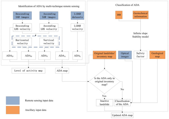
Figure 2.
Flowchart of the proposed methodology.
Firstly, the Line of Sight (LOS) displacement velocity maps and time series were derived both in ascending and descending geometry. Subsequently, InSAR LOS displacements derived from images acquired in ascending and descending orbits were converted into vertical and horizontal components by means of the module LOS2HV from ADATools [39,40,41].
Secondly, LiDAR-derived velocity was calculated, comparing both available point clouds with the multiscale model-to-model cloud comparison (M3C2) algorithm, as described in [8,42].
Third, different sets of ADAs were automatically mapped using the module ADAfinder from ADATools [39,40,41]. To this aim, five different inputs were used to generate different maps: the ascending LOS velocity that provided the ascending ADA dataset (ADAA), the descending LOS velocity map, which enabled the mapping of the ADAD, the InSAR-derived horizontal and vertical velocity maps which provided the ADAH and ADAV, respectively, and the LiDAR velocity map, from which the ADAL was derived.
Once the ADAs were identified and mapped using the different techniques, the frequency ratio method was used to calculate the number of times that every ADA was detected by the different approaches. This index can be considered as a “reliability” index of the mapped ADAs since a higher index indicates that an ADA has been detected by different techniques. In addition, the different ADAs obtained were cross-compared to build a series of confusion matrices that define the performance of the different approaches.
Finally, the ADAs were classified into different types of phenomena using ancillary information.
A detailed description of the above-described steps of the methodology is provided in the following subsections.
3.1. InSAR Processing
After data collection, the two stacks of Sentinel-1 images described in Section 2.2, covering the period from 2016 to 2021, were processed using the Sentinel Application Platform (SNAP) [43] to carry out the co-registration of the images and the generation of the interferograms. LOS displacement velocity maps of the ascending and descending orbits were processed by the Stanford Method for Persistent Scatterers (StaMPS) PSI-InSAR processing chain [44,45]. The image acquired on 6 June 2019 was selected as the reference image to process the ascending stack of images, featuring a mean-looking angle of 38.720° and a mean heading angle of 350.095°. The calculated interferograms presented a maximum spatial baseline of 130.12 m and a maximum temporal baseline of 972 days. On the other hand, the SAR image captured on 20 December 2018 was selected as the reference image to process the descending stack, featuring a mean-looking angle of 33.875° and a mean heading angle of 190.046°. The calculated interferograms had a maximum spatial baseline of 138.36 m and a maximum temporal baseline of 1056 days. A reference point located in [−0.986836W, 37.612156N] was chosen in the city of Cartagena, which was considered a stable region.
Horizontal and vertical components were computed using a reference grid with a grid spacing of 80 m, which corresponds to four times the PS size and considering the average incidence angle of the master image.
To automatically delineate the ADAs with ADAfinder, a displacement rate threshold of 3 mm/year was used in all cases. It is worth noting that the displacement rate threshold was judged according to the standard deviation of all PS velocities of the deformation map. Finally, the extent of the InSAR-derived ADAs was delineated for the four InSAR ADA maps using ADAfinder [39,40,41]. Then the four InSAR velocity maps (i.e., LOS descending, LOS ascending, horizontal, and vertical) were used to derive four ADA maps (i.e., ADAA, ADAD, ADAH, and ADAV).
3.2. LiDAR Processing
Prior to the generation of the LiDAR displacement velocity map, both point clouds were separated into ground and non-ground points. This classification was carried out by selecting a conservative ground detection method by means of the “Classify LAS ground” tool in ArcGIS [46]. Then, both point clouds were aligned in the stable area by using the iterative closest point (ICP) algorithm, which allowed obtaining the transformation matrix. It should be noted that hard rocks (e.g., dolomite, marble, dacite, and andesite) outcrops were selected as stable areas in view of the geotechnical information collected. Subsequently, the two entire point clouds were aligned by using the transformation matrix obtained in the previous step. Then, the changes between the two LiDAR acquisitions were vertically estimated from the two point clouds by means of the multiscale model-to-model cloud comparison (M3C2) in CloudCompare v2.12 software [47], which allows avoiding the need for interpolation or gridding. Finally, ground velocity values were calculated by dividing the obtained displacement by the time interval between the two acquisitions. A detailed description of the LiDAR processing method can be found in Hu et al. [8]. The resulting ground velocity map was then used to delineate the corresponding ADAs by setting a rate threshold of 3 mm/year using ADAfinder. As a result, a new ADAs map was derived from LiDAR data (ADAL).
3.3. Infinite Slope Stability Model
Slope stability is modeled in this work using an infinite slope stability model [48]. This is a simple and traditional slope stability limit equilibrium method [49] that enables to evaluate of the slope stability of a translational landslide on the soil along a planar rupture surface by means of a safety factor (SF). Despite its simplicity, the method offers the advantage that it can be easily implemented at a regional scale in a geographical information system, providing a reasonable approximation to the slope stability problem.
If we ignore the effect of vegetation on the stability of the slope, the expression for the calculation of the SF can be simplified from Escobar-Wolf et al. [50] as follows:
where:
CS is the cohesive strength of the soil.
φ is the internal friction angle of the soil.
γm is the unsaturated or moist (above the phreatic surface) soil unit weight.
γsat is the saturated (under the phreatic surface) soil unit weight.
γw is the water unit weight, a constant equal to 9.81 kN/m3 in SI units.
D is the depth of the slip surface.
HW is the height of the phreatic surface above the slip surface, normalized relative to soil thickness.
β is the terrain slope.
Note that a slope is considered unstable when SF is lower than 1.0. Moreover, we will consider the slopes poorly stable when SF varies between 1.0 and 1.2, moderately stable when SF varies between 1.2 and 1.5, and stable when SF is higher than 1.5.
In the absence of information on the depth of the slip surface, which seriously affects the slope stability, we adopted variable values from 5 to 100 m according to the range of plausible values obtained by López-Vinielles et al. [22]. Additionally, the height of the water table, which varies from completely dry (HW = 0) to completely saturated (HW = 1), represents another important factor influencing slope stability. Although previous studies [22,51] suggest that most of the time, the slopes of the study area are completely dry, we also considered the situation of saturation that might be reached in some slopes during extremely rainy weather conditions typical in this area [52]. It should be noted that although the study area presents a relatively high seismic activity [53], we only considered static conditions since no important earthquakes have struck this area during the studied period [54].
3.4. Calculation of the Level of Activity
Once the InSAR ADA maps (i.e., ADAD, ADAA, ADAH, and ADAV), the LiDAR ADA map (ADAL), and the original landslides’ inventory map were obtained, the six maps were jointly superimposed to calculate the level of activity of every ADA. The level of activity of an ADA indicates the number of times that the considered ADA has been detected by the different techniques. It ranges from 1 to 6, being 1 for those ADAs detected by only one ADA map or the original landslides’ inventory map. In contrast, for those ADAs identified in all ADA maps, including the original landslides’ inventory map, the level of activity assigned is 6. Consequently, the higher the level of activity, the higher the number of sources in which the deforming area was detected and the reliability of the active deformation area.
To evaluate the similarity and accuracy between different ADAs, the ADAs and the areas exhibiting an unstable condition in terms of safety factors were superimposed to derive two confusion matrices. The first confusion matrix analyzes the number of overlapping polygons, while the second one aims to analyze the percentage of overlap between polygons. It should be noted that only those areas with an unstable condition (i.e., with SF < 1) were taken into account for the analysis. Such areas were determined considering only the two extreme scenarios (in terms of depth of the slip surface) defined for the stability analyses, both in saturated (i.e., HW = 1 and D = 10 m; HW = 1 and D = 100 m) and unsaturated conditions (i.e., HW = 0 and D = 10 m; HW = 0 and D = 100 m). The confusion matrix that evaluates the number of times that an ADA has been detected by the different techniques can be expressed as follows:
where n is the number of ADA types (which in this case is 6, taking into account the original landslides’ inventory), m is the number of ADA types and the four different SF cases, is the overlapping number of the ADAs from the i-th ADA map with the ADAs from the j-th ADA map (i = 1, 2, …, n; j = 1, 2, …, m). If i = j, the value of is the number of ADAs of the corresponding ADA map.
The confusion matrix aimed to analyze the percentage of overlap between polygons can be expressed as follows:
where = 1, and .
3.5. Classification of ADA
The classification of the ADAs has been performed considering the capability of the remote sensing techniques to measure the displacements (e.g., large displacements, as those caused by earthworks, cannot be measured by InSAR due to the important changes in reflectivity that cause decorrelation), the characteristics of the phenomena (e.g., consolidation of waste dumps causes slow and low-magnitude displacements) and ancillary information (e.g., the original landslides’ inventory map and the SF map) (Table 2).
Table 2.
The ability of the different remote sensing techniques and the slope stability model to detect different phenomena.
Therefore, firstly, if an ADA was only included in the original landslides’ inventory map, it was classified as an inactive landslide. It was active in the past or when it was mapped by photointerpretation, but currently, it is inactive and consequently, the remote sensing techniques are not capable of capturing it.
Secondly, those ADAs that totally or partially overlapped with the original landslides’ inventory map were classified as landslides. Since they were mapped in the past and have been currently detected by remote sensing techniques, we can conclude that these ADAs are active landslides. These areas usually present a low SF in the slope stability map and important horizontal displacements.
Thirdly, if an ADA is detected by remote sensing techniques but is not mapped in the original landslides’ inventory map, then we do not have previous information about the underlying phenomenon. Then, we can perform a preliminary classification of the ADA using the available ancillary information (i.e., the SF map, the geological map, and the orthophotos), considering the capability of remote sensing techniques to measure the displacements expected for every different phenomenon (Table 2).
Those ADAs derived from InSAR, LiDAR, or both, partially placed over areas exhibiting SF values lower than one in the slope stability map, can be classified as probable landslides. These areas usually exhibit important horizontal displacements. We also should take into account that landslides can develop on waste dumps (i.e., tailing dumps), slopes of open pit mines, and natural slopes mapped in the geological map.
When an ADA is only detected by LiDAR (i.e., it is included in the ADAL map) but not by InSAR, a high or quick mass loss or gain (e.g., erosion or earthworks) could be the cause of the loss of the interferometric coherence, which prevents their monitoring by means of InSAR. More specifically, erosion mainly develops in steep areas, and the magnitude of the phenomenon is usually a few centimeters or decimeters in the study area. It can develop on the open pit slopes, waste dump slopes, and natural slopes represented in the geological map. Complementarily, earthworks cause very big changes (even of several meters). Both erosion and earthworks are easily recognizable in the optical images.
Those ADAs not mapped in the ADAL but in the ADAs derived from InSAR, or those ADAs mapped by both techniques which exhibit a high SF, correspond to small magnitude gradual processes such as waste dump consolidation or subsidence. The main difference between both phenomena is that consolidation develops on areas of accumulated soil, as waste dumps or areas of the previous filling (after earthworks), which can be easily identified in optical images and are mapped in the geological map.
Finally, some of the above-mentioned processes can overlap in space and time. For example, mining waste deposits can be affected by consolidation processes, as well as landslides and erosion near the slopes. In these cases, differentiating the extent of the different processes is not possible, and then, they are pre-classified as compound processes.
It should be noted that there is a probability that the ADAs, which theoretically should be detected by InSAR and LiDAR, are missing due to different issues (e.g., atmospheric, and unwrapping errors or insensitivity to northwards and southwards displacements for InSAR), which will affect the judgment.
Furthermore, some ADAs detected by LiDAR can be associated with changes in the vegetation cover or in the water level of mining lakes but not with a deformational geological-geotechnical process. Consequently, these ADAs are classified as false ADAs.
Moreover, it is worth mentioning that this methodology must be considered as a pre-classification procedure for wide areas and thus, further expert analysis and in situ work is necessary to confirm the deformation process underlying each ADA.
4. Results and Analyses
4.1. InSAR-Derived ADA Maps
As described in the previous section, four ADA maps were directly derived from the InSAR-derived ground deformation results. Thus, an ascending LOS ADA map (ADAA), a descending LOS ADA map (ADAD), a horizontal ADA map (ADAH), and a vertical ADA map (ADAV) were obtained (Figure 3). Note that negative values (red color) in Figure 3a,b,d represent the movements away from the sensor, whereas positive values (blue color) represent the movements toward the radar. In contrast, negative values (red color) in Figure 3c represent westward movement, whereas positive values (blue color) indicate eastward movement. Furthermore, the LOS velocity thresholds selected to represent the stable points in Figure 3 were set at +5 and −5 mm/year.
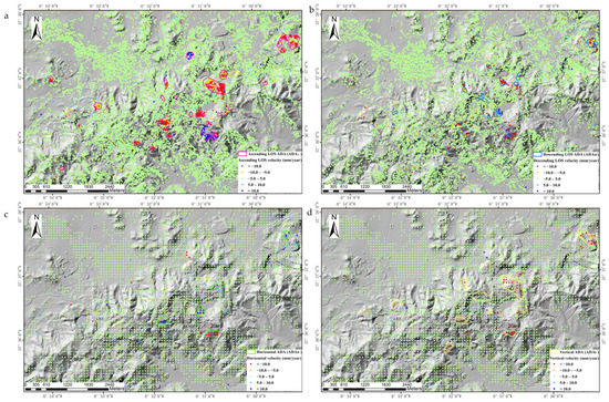
Figure 3.
InSAR ascending LOS velocity map (a), descending LOS velocity map (b), horizontal (east-west) velocity map (c) and vertical velocity map (d) for the period from October 2016 to November 2021. The pink solid polygons, blue solid polygons, green solid polygons and yellow solid polygons indicate the boundaries of the ADAA, ADAD, ADAH and ADAV, respectively.
As shown in Figure 3a,b, 28 and 19 active areas were derived from the ascending (ADAA) and descending (ADAD) ground velocity maps, respectively.
Although both LOS velocity maps allow us to define the location and the spatial extent of each of the mapped ADAs, it is hard to determine the contributions of the horizontal and vertical components of the displacements by using LOS displacement velocities. In order to overcome this limitation, the two LOS velocity maps were used to generate both a horizontal and a vertical velocity map, from which two sets of ADAs were derived. Figure 3c,d show the two-dimensional (2D) displacement velocity maps obtained in an east-west and vertical direction, respectively. A total of 5 and 12 ADAs were derived from the horizontal and vertical ground deformation maps (ADAH and ADAV), respectively. It should be noted that since the LOS InSAR data were gridded in order to calculate the vertical and horizontal components, there are some ADAs not detected by ADAA and ADAD, which, however, have been detected in ADAH and ADAV.
4.2. LiDAR-Derived ADA Map
Figure 4 shows the LiDAR vertical velocity map calculated for the whole area as described in Section 3.2. Note that negative values (red color) represent downward movement, whereas positive values (blue color) indicate upward movement. It should also be noted that the velocity thresholds selected to represent the stable points in Figure 4 were likewise set at +5 and −5 mm/year. A total of 58 ADAs derived from this map (ADAL) are also depicted in Figure 4 as black polygons.
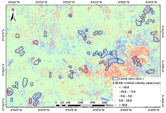
Figure 4.
LiDAR vertical velocity map for the period 2009–2016 and detected ADAs.
4.3. Safety Factor Map
The safety factor (SF), which is calculated by means of Equation (1) for an infinite slope failure, indicates how close the analyzed slopes are to the threshold for a failure to occur. It depends on several geometrical, hydrological, and geomechanical variables. These include, among others, variables such as the depth of the slip surface and the normalized height of the phreatic surface above the slip surface, whose values were completely unknown in the investigated case study. In this work, in order to address these uncertainties, the safety factor maps were computed considering a variable range of values of depth of the slip surface derived from the available literature and two extreme scenarios of pore water pressure (a fully saturated scenario, and a completely dry scenario, the former corresponding to an extreme rainfall situation).
Thus, stability analyses were conducted using a thickness of the soil layer varying from 5 to 100 m. The results obtained using a depth of the slip surface of 5 m reveal that the whole area is stable (i.e., SF > 1), as shown in Table 3 and Figures S1 and S2. This suggests that the area is not susceptible to suffering shallow planar failures. However, as revealed by the analyses conducted using higher soil thickness values, the number of unstable areas (SF < 1) gradually increases with the increase in the depth of the slip surface (Table 3 and Figures S1 and S2).
Table 3.
Distribution of areas featuring an unstable (safety factor SF < 1.0), a poorly stable (1.0 ≤ SF < 1.2), a moderately stable (1.2 ≤ SF < 1.5), and a stable (SF ≥ 1.5) behavior for the two groundwater scenarios considered (HW equal either to 0 or 1) and for depth values of the slip surface (D) varying from 5 to 100 m.
As previously mentioned, the height of the phreatic surface above the slip surface (HW), normalized relative to soil thickness, was set at either 0 (dry) or 1 (saturated) in order to account for the two extreme hydrological scenarios. Although La Union is a very dry area [52], HW could be increased during the rainy seasons and extreme weather. Therefore, two different groundwater conditions were considered by fixing a phreatic ratio value of either 0 or 1. As shown in Table 3 and Figures S1 and S2, the average SF is considerably reduced when HW = 1 and the total unstable area (i.e., that exhibiting an SF < 1) is much greater than that calculated for HW = 0. In addition, the spatial variation of the safety factor results with D can be clearly seen for HW = 0 and HW = 1 in Figure 5a,b.
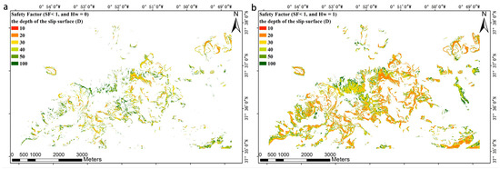
Figure 5.
Distribution of areas exhibiting a safety factor lower than 1 in dry conditions (HW = 0) (a) and in saturated conditions (HW = 1) (b) considering depth values of the slip surface (D) varying from 10 to 100 m.
Figure 5 shows the spatial distribution of the areas exhibiting a safety factor lower than 1 (i.e., the unstable areas). According to these results, it was spatially confirmed that the deeper the depth of the slip surface (D), the larger the unstable region, regardless of the value of HW. Moreover, the results revealed that failures are more likely to be triggered with increasing values of HW.
4.4. Level of Activity Map
As previously described, the level of level activity map activity map was generated by superimposing and merging the five ADA maps obtained (ADAA, ADAD, ADAH, ADAV, and ADAL) on the original landslides’ inventory map. The map thus obtained yielded 100 ADAs (Figure S3), out of which 2 correspond to level 6, 4 to level 5, 4 to level 4, 4 to level 3, 10 to level 2, and 76 to level 1 (Figure 6a). Note that the higher the level of activity of instability, the higher number of maps in which the active deformation area was detected. Therefore, as explained above, this parameter can be considered as a proxy of the probability that such instability is not a false positive. Consequently, the higher the level of activity, the more reliable the detected active deformation area.
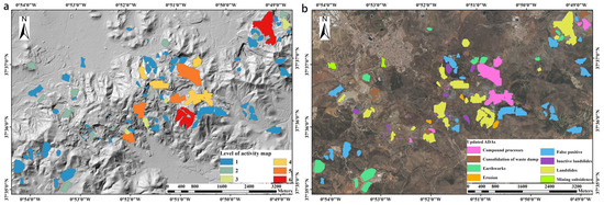
Figure 6.
(a) Level of activity map of the updated inventory map. (b) Classification of the ADA of the updated inventory map according to the underlying deformation process.
4.5. Classification and Updated ADA Map
After this performance assessment, the detected instabilities were classified into different types of deformation phenomena (Figure 6b and Table 4) on the basis of the results derived from the ADA maps, the SF maps, and some ancillary information, basically consisting of a geological map and a series of optical images. Figures S4–S8 show some examples of different ADAs mapped on the study area.
Table 4.
Statistical distribution of the type of phenomena causing displacements.
A total of 29 out of the instabilities included in the original inventory map were neither detected by InSAR nor by LiDAR, which suggests that such instabilities were active between 1996 and 2010 (the period covered by the original inventory map), remaining stable for the time periods covered by the ADA maps. Instabilities detected by either the InSAR or the LiDAR ADA maps were classified as described in the methodology (Section 3.5).
5. Discussion
5.1. Comparison of the Results Obtained Using the Different Techniques
In order to evaluate the performance of the different ADAs, two confusion matrices were derived by superimposing the inventoried landslides, the ADAs, and the areas exhibiting an unstable condition (i.e., with SF < 1). The two confusion matrices were generated considering only the two extreme case scenarios (in terms of depth of the slip surface) defined for the stability analyses, both in saturated and unsaturated conditions. Four different scenarios (i.e., HW = 0, D = 10 m; HW = 1, D = 10 m; HW = 0, D = 100 m; and HW = 1, D = 100 m) were thus taken into account. First, a confusion matrix was obtained to analyze the overlapping number of polygons (Table 5). Then, an additional confusion matrix was derived from the former to analyze the overlapping rate of polygons (Table 6).
Table 5.
Confusion matrix to analyze the overlapping number of polygons.
Table 6.
Confusion matrix to analyze the percentage overlap between polygons.
It is worth noting that the original landslides’ inventory map, the LiDAR-derived ADAs, and the InSAR-derived ADAs cover slightly different time periods with short common time periods. Consequently, only those active deformation areas remaining active between 2010 (i.e., the date in which the original inventory map was updated) and 2022 (i.e., the last date covered by InSAR) can be commonly mapped by the three approaches considered in this work (i.e., photointerpretation and field work performed for the mapping of the landslides’ inventory map, InSAR processing, and LiDAR processing). On the other hand, it has to be taken into account that some of the ADAs detected are related to processes other than landslides (e.g., waste dump consolidation, earthworks, etc.), and thus they are not mapped in the original landslides’ inventory map leading to differences between the compared maps. In contrast, the use of information from different temporal periods presents the benefit of offering the possibility of evaluating the activity of the landslides mapped in the original landslides’ inventory map as well as detecting new active processes not included in the original inventory.
As shown in Table 5 and Table 6, the comparison of the original landslides’ inventory map with the five ADA maps obtained by applying the proposed methodology shows that the ADAA map features the largest number of overlaps, with 34 matches and a match rate of 41.46%. In addition, the comparison of the ADA maps with the original landslides’ inventory indicates that although the ADAA map features the maximum number of matches (a total of 16) as well, in this case, the ADAH map features the highest match rate, with a value of 100%. Table 5 also shows that the ADAL map yields the highest number of ADAs, with a total of 58. Considering only the ADAs, the maximum overlapping number of polygons is obtained by comparing the ADAD map with the ADAA, a total of 14 overlaps. Furthermore, the highest overlapping rate (100%) is obtained by comparing the ADAH map with the ADAA, whereas the lowest overlapping rate (8.62%) is obtained by comparing ADAL with ADAD and ADAH.
As previously mentioned, the difference observed among the different ADA maps obtained through the application of the proposed methodology are related not only to the fact that the five maps cover different time periods but also to the different acquisition geometries and special coverages associated with maps. In addition to the reasons mentioned above for the different time periods, there are other reasons. Firstly, SAR data are acquired along the ascending or descending LOS, while LiDAR data are always acquired in the vertical direction. For this reason, in mountainous areas, the InSAR results obtained in ascending geometry often considerably differ, in terms of spatial coverage, from those obtained in descending geometry. This constitutes an important limitation in relation to the application of ADAfinder since the algorithm implemented by the tool applies an aggregation procedure that delineates the ADAs using a minimum number of points, which must be defined by the user. Thus, when the number of active points in a given area is lower than the selected value, the points are ignored by ADAfinder, and no ADA is obtained.
Finally, the comparison of the original landslides’ inventory map with the unstable areas reveals that the overlapping number of polygons obtained for D = 100 m far exceeds the one obtained for D = 10 m. On the other hand, the comparison of the ADA maps with unstable areas reveals that ADAL features the maximum overlapping number. As shown in Table 5, the number of overlaps between the original landslides’ inventory map and the unstable areas results in 13 and 66 for D, equal to 10 and 100 m, respectively (regardless of the value of HW). When focusing on the ADAs, the results also show that overlapping numbers of polygons obtained with D = 10 m for each of the ADA maps are identical, regardless of the value of HW. In any event but except for ADAD and ADAL, the overlaps obtained with D = 100 m show a negligible difference, which means that the results obtained for each ADA map are identical regardless of the value of HW. These results suggest that the depth of the slip surface D plays a key role in the stability of the slopes, while the soil phreatic ratio HW seems to act as a triggering factor.
5.2. Characteristics of the Different Technologies for the Detection and Classification of ADAs
In this section, the main advantages and drawbacks of the techniques used to map and classify the active deformation areas summarized in Table 7 are discussed in detail.
Table 7.
Comparison of the main features of the different techniques used for the detection and classification of ADAs.
LiDAR is characterized by its ability to delineate rapid and large-gradient movements (e.g., erosion and earthwork) in a detailed way due to the high density of points (i.e., 0.5 points per square meter) acquired through a vertical geometry (see, for example, Figures S4 and S8). In contrast, InSAR enables the detection of slow and small displacements (e.g., consolidation of the waste dump) along the LOS of the satellite and in the vertical and east-west directions, with high accuracy and a wide number of images due to the high temporal sampling (Figures S5–S7). It should be highlighted that both remote sensing techniques are time-consuming due to the wide number of processes that should be performed to obtain the final datasets. Furthermore, by analyzing the results obtained, it was found that the boundaries of the LiDAR-derived ADAs matched much better (compared to those obtained with InSAR) the actual boundaries of the originally mapped instabilities. Thus, the use of LiDAR data not only leads to an increase in the number of mapped ADAs but also to a more detailed delineation of the actual boundaries of the instabilities.
LiDAR has the ability to penetrate vegetation, but there are still many spots reflecting from the vegetation surface [55]. The dense vegetation is mostly located in mountainous areas, in which it is more difficult to distinguish between ground points and vegetation surface points. Therefore, LiDAR is sensitive to changes in dense vegetation. Although the study area is scarcely vegetated and non-ground points were removed from the original point clouds, LiDAR datasets have captured some possible ADAs (e.g., 4, 5, 8, and 16 in Figure S3) that could be related to vegetation changes instead of ground surface displacements leading to false positives (Figure S8). Similarly, a false positive related to the variation of water level changes due to groundwater rise and the contribution of surface water from streams in a mining lake resulting in an abandoned open pit mine [56] has been found in ADA 19. In these cases, in situ inspection is crucial to confirm the ADAs. In contrast, InSAR datasets decorrelate on vegetated and flooded areas, and thus, no ADAs have been detected in these places.
The slope stability model is not a detection technique itself but provides very useful ancillary information for the classification of potential landslide areas exhibiting an SF lower than 1 (Figures S7 and S8). However, it should be noted that this information is strongly affected by the uncertainties in the input data (e.g., geotechnical parameters, failure depth, or hydrological conditions), although it is easy and simple to apply, providing a valuable simplification of the slope instability problem.
Optical images can be effectively used for the identification and mapping of geomorphological features (e.g., tension cracks and scarps of a landslide) and landforms (e.g., earthworks as the construction of a filling or an excavation) associated with active deformations areas. They complement the information of the geological map, which contains different mining facilities (Figures S5 and S6). However, the interpretation of optical images is a very time-consuming task that requires important expertise. Furthermore, cloud and fog, abnormal bands and color, texture clarity, and other image quality issues strongly affect their quality and even sometimes obstruct the view of the ground surface, preventing the mapping of the geomorphological features and landforms.
5.3. Uncertainties of the Method
As described above, mining areas constantly change and evolve. A lot of different processes develop at the same time and can overlap in time and space. The methodology established in this work enables the identification and mapping of active deformation areas in mining regions exploiting the complementarities of LiDAR and InSAR techniques.
As it is well known, InSAR data are affected by different sources of error (e.g., atmospheric delay, topographic residuals, processing approximations, timing errors, and hardware issues) [57]. Similarly, LiDAR datasets are also affected by distinct error sources (e.g., cloud co-registration, georeferencing, and editing) [58]. Furthermore, changes due to non-geological-geotechnical causes (e.g., the growth of vegetation or water level changes in mining lakes) can induce false positives. Consequently, all these sources of error can lead to the identification of unreliable deforming areas in mining areas.
Therefore, the joint use of LiDAR and InSAR exploits the complementarities and similarities of both techniques to update ADAs maps in mining areas, making the process of identification more robust and reliable when the mapped active deformation areas are redundant. In contrast, in those ADAs only captured by one of the techniques, the degree of uncertainty will strongly depend on the quality of the LiDAR or InSAR dataset (i.e., of the inherent uncertainties of the input datasets). In these cases, further ancillary data and/or in situ information can allow the confirmation of the reliability of the detected ADA. Consequently, we recommend using the level of activity of the ADAs as a reliability index.
Some uncertainties can also arise during the process of preliminary classification of the ADAs. When the ADAs are compared to the original landslides’ inventory map, the classification is straightforward since the landslides that overlap the ADA have been previously confirmed on the field and through optical images. However, for the rest of the ADAs, ancillary information must be used, and some conditions are assumed, introducing some uncertainties in the classification. Optical images can play an important role in reducing the uncertainties that arise during the classification process since they enable the identification of key geomorphological features and landforms.
We should also take into account that different processes can overlap over time and space, hampering the classification of ADAs. For example, in Figure S8c,d, surface erosion and a landslide seem to be affecting a waste dump in which an ADA was detected by LiDAR. In these cases, the subsequent fieldwork and in situ monitoring are necessary to state the actual underlying phenomena causing the measured displacements.
In summary, this method allows the exploitation of the synergies between the different techniques to detect and delineate active areas (i.e., areas that are moving) to update existing inventory maps. Then, the ADAs are pre-classified by analyzing the LiDAR and InSAR datasets, the landslides’ inventory map, the safety factor map, and the optical images. However, fieldwork and even in situ monitoring would be necessary to definitively confirm the previous classification and reduce the uncertainties that arose during the identification and classification processes since only the ADAs overlapped with the original landslides’ inventory map could be confirmed as reliable.
6. Conclusions
The mining area of Sierra de Cartagena-La Union has been affected by multiple deformation processes (e.g., slope deformation, waste dump consolidation, and soil erosion) since the mining activity in the region ceased in 1991. These processes are potentially hazardous for populations and infrastructures and, therefore, require early identification.
In this work, we propose a novel multi-technique approach combining InSAR-derived and LiDAR-derived ground velocity maps together with a slope safety factor map, a geological map, and aerial images to identify active deformation areas and update inventory maps in mining areas. It is worth stressing that this is the first time that ADA methodology is applied to automatically analyze LiDAR-derived change detection maps, expanding this type of analysis to the field of LiDAR.
The proposed methodology enabled the generation of five comprehensive ADAs maps. A total of 28, 19, 5, and 12 ADAs were mapped using InSAR deformation results derived from ascending and descending datasets, and horizontal and vertical deformation components, respectively. Additionally, 58 ADAs were derived from LiDAR vertical velocity data. The joint analysis of the ADAs derived from the different remote sensing techniques and an existing landslides’ inventory map enabled the calculation of a map of the level of activity, which is a proxy for the evaluation of the reliability of the mapped ADAs.
Then, the slope stability was systematically analyzed over the study area for different depths of the slip surface (D) and soil phreatic ratio (HW) values by adopting an infinite slope stability modeling approach. Finally, all instabilities detected were classified into different types of deformation processes considering the original landslides’ inventory map, the SF map, the geological map, and the photointerpretation aerial images. A total of 8, 11, 3, 17, 2, and 7 ADAs were classified as consolidation of the waste dump, earthworks, erosion, landslides, mining subsidence, and compound processes, respectively.
The general conclusions drawn from this work can be summarized as follows: (i) The joint use of InSAR and LiDAR techniques to map ADAs improves the capability to detect different types of phenomena in mining areas due to the exploitation of the complementarities of both techniques. LiDAR can play a significant role in the detection of rapid and huge ground movements, such as those induced by earthworks and erosion. In contrast, the InSAR technique presents an advantage in the detection of smaller and slow vertical and horizontal movements. (ii) The infinite slope stability modeling approach is an effective means to generate SF maps, which can be used as complementary information, jointly with the geological maps and optical images, for the identification and classification of ADAs prone to landslides. (iii) Some unavoidable uncertainties arise during the identification and classification of the ADAs. Consequently, the InSAR-derived maps, the LiDAR-derived maps, and the original landslides’ inventory map were used to build a map of the level of activity that considers the overlapping number of ADAs, providing an estimation of the reliability of every ADA.
Finally, it should be highlighted that the methodology established enables the semiautomatic identification and mapping of active deformation areas in mining regions using huge remote sensing datasets and their preliminary classification. However, the final confirmation of the underlying processes will require the availability of field information and expert opinion. The results derived through the proposed methodology will considerably facilitate the management and the subsequent analysis of a huge amount of information and data available in mining areas.
Supplementary Materials
The following supporting information can be downloaded at: https://www.mdpi.com/article/10.3390/rs15040996/s1, Figure S1: Safety factor map computed by the infinite slope stability model in dry conditions (height of phreatic surface above slip surface, normalized relative to soil thickness, HW equal to 0) for depth values of the slip surface (D) varying from 10 to 100 m. Figure S2: Safety factor map computed by the infinite slope stability model in saturated conditions (height of phreatic surface above slip surface, normalized relative to soil thickness, Hw equal to 1) for depth values of the slip surface (D) varying from 10 to 100 m. Figure S3: Map of distribution of updated ADAs. Figure S4: ADA associated to earthworks: (a,c) Optical images of the ADA 24 (see location in Figure S3) from 2007 and 2016, respectively, in which the earthworks performed are clearly recognized. (b) LiDAR changes and contour of the ADAL. Note that the magnitude of the changes reach up to −3 m in some areas of the ADA. (d) Shaded relief map with the updated contour of ADA 24. Figure S5: ADA associated to the consolidation of a waste dump: (a,c) Optical images of the ADA 69 (see location in Figure S3) from 2016 and 2020, respectively. (b) InSAR displacements map and contour of the ADAA and ADAV. (d) Geological map of the ADA. (e) Time series of the ADA in which the gradual attenuation of the settlements is clearly recognized. Figure S6: ADA associated to mining subsidence: (a) 3D view of the ADA 76 (see location in Figure S3). (b) LiDAR results between 2009 and 2016 including the updated ADA contour. (c) Picture of a headframe placed within ADA 76. (d) Picture of an earth fissure identified on the ground surface of ADA 76 related to mining subsidence. (e) InSAR displacements map and contour of the updated ADA. (f) Geological map of the ADA. (g) Shaded relief map of the ADA 76 with the contours of the ADAs detected by LiDAR (ADAL) and InSAR (ADAA). Figure S7: ADA associated to a landslide: (a) 3D view of the ADA 66 (see location in Figure S3). (b) InSAR time series of some points placed within and out of the ADA. See location of the points in Figure S7d. (c) Shaded relief map with the contour of the ADAs detected by InSAR (ADAA), the landslide mapped in the original landslides’ inventory map, and the safety factor calculated by means of the infinite slope model. (d) InSAR displacements map and contour of the updated ADA. Figure S8: Safety factor map and landslide contour of ADA 47 (see location in Figure S3) (a) and InSAR ascending and descending results mapped in the original landslides’ inventory map (b). 3D view with indication of some geomorphological features of the underlying processes (c) and LiDAR results (d) of ADA 3 (see location in Figure S3) affected by a landslide and erosion. 3D view of a possible false positive ADA (e) and its LiDAR results (f) (ADA 16; see location in Figure S3).
Author Contributions
L.H. performed the experiments and produced the results. L.H. and R.T. drafted the manuscript, and X.T. finalized the manuscript. G.H. and J.L.V. provided the geological material and guided outline of this paper. X.T., R.T., J.L.V., G.H., T.L. and Z.L. contributed to the discussion of the results. All authors have read and agreed to the published version of the manuscript.
Funding
This research was funded by the ESA-MOST China DRAGON-5 project (ref. 59339) and funded by a Chinese Scholarship Council studentship awarded to Liuru Hu (Ref. 202004180062).
Data Availability Statement
The Sentinel-1 datasets used in this study were freely downloaded from Copernicus and ESA, and the DEM data were freely downloaded from the website https://centrodedescargas.cnig.es/CentroDescargas/index.jsp (accessed on 1 July 2022). The LiDAR datasets and orthophotos used in this work were freely downloaded from the Centro Nacional de Información Geográfica (CNIG) del Instituto Geográfico Nacional (IGN) de España (https://www.cnig.es/) (accessed on 1 July 2022).
Acknowledgments
The authors would like to thank Joaquín Mulas from the Instituto Geológico y Minero de España (IGME) for providing a technical report of the study area. The figures in this study were prepared using Matlab R2021a and QGIS 3.22. LiDAR datasets were processed using CloudCompare and ArcGIS.
Conflicts of Interest
The authors declare no conflict of interest.
References
- Tomás, R.; Romero, R.; Mulas, J.; Marturià, J.J.; Mallorquí, J.J.; López-Sánchez, J.M.; Herrera, G.; Gutiérrez, F.; González, P.J.; Fernánde, J.; et al. Radar Interferometry Techniques for the Study of Ground Subsidence Phenomena: A Review of Practical Issues through Cases in Spain. Environ. Earth Sci. 2013, 71, 163–181. [Google Scholar] [CrossRef]
- Kyriou, A.; Nikolakopoulos, K. Landslide mapping using optical and radar data: A case study from Aminteo, Western Macedonia Greece. Eur. J. Remote Sens. 2020, 53, 17–27. [Google Scholar] [CrossRef]
- Samsonov, S.; d’Oreye, N.; Smets, B. Ground deformation associated with post-mining activity at the French–German border revealed by novel InSAR time series method. Int. J. Appl. Earth Obs. Geoinf. 2013, 23, 142–154. [Google Scholar] [CrossRef]
- Carlà, T.; Farina, P.; Intrieri, E.; Ketizmen, H.; Casagli, N. Integration of ground-based radar and satellite InSAR data for the analysis of an unexpected slope failure in an open-pit mine. Eng. Geol. 2018, 235, 39–52. [Google Scholar] [CrossRef]
- Xiaojie, L.; Zhao, C.; Zhang, Q.; Lu, Z.; Li, Z.; Yang, C.; Zhu, W.; Liu-Zeng, J.; Chen, L.; Liu, C. Integration of Sentinel-1 and ALOS/PALSAR-2 SAR datasets for mapping active landslides along the Jinsha River corridor, China. Eng. Geol. 2021, 284, 106033. [Google Scholar] [CrossRef]
- Ferretti, A.; Savio, G.; Barzaghi, R.; Borghi, A.; Musazzi, S.; Novali, F.; Prati, C.; Rocca, F. Submillimeter Accuracy of Insar Time Series: Experimental Validation. Geosci. Remote Sens. 2007, 45, 1142–1153. [Google Scholar] [CrossRef]
- Bernard, T.; Lague, D.; Steer, P. Beyond 2D landslide inventories and their rollover: Synoptic 3D inventories and volume from repeat lidar data. Earth Surf. Dyn. 2021, 9, 1013–1044. [Google Scholar] [CrossRef]
- Hu, L.; Navarro-Hernández, M.I.; Liu, X.; Tomás, R.; Tang, X.; Bru, G.; Ezquerro, P.; Zhang, Q. Analysis of regional large-gradient land subsidence in the Alto Guadalentín Basin (Spain) using open-access aerial LiDAR datasets. Remote Sens. Environ. 2022, 280, 113218. [Google Scholar] [CrossRef]
- Scott, C.; Phan, M.; Nandigam, V.; Crosby, C.; Arrowsmith, R. Measuring change at Earth’s surface: On-demand vertical and three- dimensional topographic differencing implemented in OpenTopography. Geosphere 2021, 17, 1318–1332. [Google Scholar] [CrossRef]
- Borsa, A.; Minster, J.B. Rapid Determination of near-Fault Earthquake Deformation Using Differential Lidar. Bull. Seismol. Soc. Am. 2012, 102, 1335–1347. [Google Scholar] [CrossRef][Green Version]
- Scott, C.; Champenois, J.; Klinger, Y.; Nissen, E.; Maruyama, T.; Chiba, T.; Arrowsmith, R. 2016 M7 Kumamoto, Japan, Earthquake Slip Field Derived from a Joint Inversion of Differential Lidar Topography, Optical Correlation, and Insar Surface Displacements. Geophys. Res. Lett. 2019, 46, 6341–6351. [Google Scholar] [CrossRef]
- Okyay, U.; Telling, J.; Glennie, C.L.; Dietrich, W.E. Airborne Lidar Change Detection: An Overview of Earth Sciences Applications. Earth-Sci. Rev. 2019, 198, 102929. [Google Scholar] [CrossRef]
- Brock, J.C.; Sallenger, A.H.; Krabill, W.B.; Swift, R.N.; Wright, C.W. Recognition of Fiducial Surfaces in Lidar Surveys of Coastal Topography. Photogramm. Eng. Remote Sens. 2001, 67, 1245–1258. [Google Scholar]
- Bull, J.M.; Miller, H.; Gravley, D.M.; Costello, D.; Hikuroa, D.C.H.; Dix, J.K. Assessing Debris Flows Using Lidar Differencing: 18 May 2005 Matata Event, New Zealand. Geomorphology 2010, 124, 75–84. [Google Scholar] [CrossRef]
- Mora, O.E.; Lenzano, M.G.; Toth, C.K.; Grejner-Brzezinska, D.A.; Fayne, J.V. Landslide Change Detection Based on Multi-Temporal Airborne Lidar-Derived Dems. Geosciences 2018, 8, 23. [Google Scholar] [CrossRef]
- Liu, X. Airborne Lidar for Dem Generation: Some Critical Issues. Prog. Phys. Geogr. 2008, 32, 31–49. [Google Scholar]
- Treitz, P.; Lim, K.; Woods, M.; Pitt, D.; Nesbitt, D.; Etheridge, D. Lidar Sampling Density for Forest Resource Inventories in Ontario, Canada. Remote Sens. 2012, 4, 830–848. [Google Scholar] [CrossRef]
- Estornell, J.; Ruiz, L.A.; Velázquez-Martí, B.; Hermosilla, T. Analysis of the Factors Affecting Lidar Dtm Accuracy in a Steep Shrub Area. Int. J. Digit. Earth 2011, 4, 521–538. [Google Scholar] [CrossRef]
- Liu, J.; Liu, X.; Lv, X.; Wang, B.; Lian, X. Novel Method for Monitoring Mining Subsidence Featuring Co-Registration of Uav Lidar Data and Photogrammetry. Appl. Sci. 2022, 12, 9374. [Google Scholar] [CrossRef]
- Zhang, Y.; Lian, X.; Ge, L.; Liu, X.; Du, Z.; Yang, W.; Wu, Y.; Hu, H.; Cai, Y. Surface Subsidence Monitoring Induced by Underground Coal Mining by Combining Dinsar and Uav Photogrammetry. Remote Sens. 2022, 14, 4711. [Google Scholar] [CrossRef]
- Lucieer, A.; Jong, S.M.D.; Turner, D. Mapping Landslide Displacements Using Structure from Motion (Sfm) and Image Correlation of Multi-Temporal Uav Photography. Prog. Phys. Geogr. 2013, 38, 97–116. [Google Scholar] [CrossRef]
- López-Vinielles, J.; Fernández-Merodo, J.A.; Ezquerro, P.; García-Davalillo, J.C.; Sarro, R.; Reyes-Carmona, C.; Barra, A.; Navarro, J.A.; Krishnakumar, V.; Alvioli, M.; et al. Combining Satellite InSAR, Slope Units and Finite Element Modeling for Stability Analysis in Mining Waste Disposal Areas. Remote Sens. 2021, 13, 2008. [Google Scholar] [CrossRef]
- Herrera, G.; Tomás, R.; Vicente-Guijalba, F.; Lopez-Sanchez, J.; Mallorqui, J.; Mulas, J. Mapping ground movements in open pit mining areas using differential SAR interferometry. Int. J. Rock Mech. Min. Sci. 2010, 47, 1114–1125. [Google Scholar] [CrossRef]
- Lopez Gayarre, F.; Álvarez-Fernández, M.I.; González Nicieza, C.; Álvarez-Vigil, A.E.; Herrera, G. Forensic analysis of buildings affected by mining subsidence. Eng. Fail. Anal. 2010, 17, 270–285. [Google Scholar] [CrossRef]
- Herrera, G.; Tomás, R.; Lopez-Sanchez, J.; Delgado, J.; Mallorqui, J.; Duque, S.; Mulas, J. Advanced DInSAR analysis on mining areas: La Union case study (Murcia, SE Spain). Eng. Geol. 2007, 90, 148–159. [Google Scholar] [CrossRef]
- Álvarez-Vigil, A.E.; González-Nicieza, C.; López Gayarre, F.; Álvarez-Fernández, M.I. Forensic analysis of the evolution of damages to buildings constructed in a mining area (Part II). Eng. Fail. Anal. 2010, 17, 938–960. [Google Scholar] [CrossRef]
- Herrera, G.; Álvarez-Fernández, M.I.; Tomás, R.; González Nicieza, C.; Lopez-Sanchez, J.; Álvarez-Vigil, A.E. Forensic analysis of buildings affected by mining subsidence based on Differential Interferometry (Part III). Eng. Fail. Anal. 2012, 24, 67–76. [Google Scholar] [CrossRef]
- Álvarez-Fernández, M.I.; Álvarez-Vigil, A.E.; González-Nicieza, C.; López Gayarre, F. Forensic evaluation of building damage using subsidence simulations. Eng. Fail. Anal. 2011, 18, 1295–1307. [Google Scholar] [CrossRef]
- Alvarez-Garcia, I.N.; Ramos-Lopez, F.L.; Gonzalez-Nicieza, C.; Alvarez-Fernandez, M.I.; Alvarez-Vigil, A.E. The mine collapse at Lo Tacón (Murcia, Spain), possible cause of the Torre Pacheco earthquake (2nd May 1998, SE Spain). Eng. Fail. Anal. 2013, 28, 115–133. [Google Scholar] [CrossRef]
- Manteca, J.; Ovejero, G. Los Yacimientos Zn, Pb, Ag-Fe del Distrito Minero de la La Unión-Cartagena, Bética Oriental; CSIC: Madrid, Spain, 1992. [Google Scholar]
- Robles-Arenas, V.M.; Rodríguez, R.; García, C.; Manteca, J.I.; Candela, L. Sulphide-mining impacts in the physical environment: Sierra de Cartagena–La Unión (SE Spain) case study. Environ. Geol. 2006, 51, 47–64. [Google Scholar] [CrossRef]
- Conesa, H.M.; Schulin, R.; Nowack, B. Mining landscape: A cultural tourist opportunity or an environmental problem?: The study case of the Cartagena–La Unión Mining District (SE Spain). Ecol. Econ. 2008, 64, 690–700. [Google Scholar] [CrossRef]
- Instituto Geológico y Minero de España (IGME). Estudio Geotécnico para el Depósito de Residuos de la Bahía de Portman en Corta Minera, Madrid; Instituto Geológico y Minero de España: Madrid, Spain, 1996. [Google Scholar]
- IGN. Plan Nacional de Ortografía Aérea (PNOA). Available online: https://pnoa.ign.es/estado-del-proyecto-lidar (accessed on 1 March 2022).
- CNIG. Digital Elevation Models. 2022. Available online: https://centrodedescargas.cnig.es/CentroDescargas/locale?request_locale=en (accessed on 1 July 2022).
- Monterroso Checa, A. Remote sensing and archaeology from Spanish LiDAR-PNOA: Identifying the amphitheatre of the roman city of torreparedones (Córdoba-Andalucía-Spain). Mediterr. Archaeol. Archaeom. 2017, 17, 15–22. [Google Scholar] [CrossRef]
- IGN. Altimetric Precision Control Information of the Als Campaign Performed in 2009; Internal Report; Instituto Geográfico Nacional: Madrid, Spain, 2009. [Google Scholar]
- IGN. Altimetric Precision Control Information of the Als Campaign Performed in 2016; Internal Report; Instituto Geográfico Nacional: Madrid, Spain, 2016. [Google Scholar]
- Navarro, J.; Tomás, R.; Barra, A.; Pagán, J.; Reyes-Carmona, C.; Solari, L.; Lopez Vinielles, J.; Falco, S.; Crosetto, M. ADAtools: Automatic Detection and Classification of Active Deformation Areas from PSI Displacement Maps. Int. J. Geo-Inf. 2020, 9, 584. [Google Scholar] [CrossRef]
- Tomás, R.; Pagán, J.I.; Navarro, J.A.; Cano, M.; Pastor, J.L.; Riquelme, A.; Cuevas-González, M.; Crosetto, M.; Barra, A.; Monserrat, O.; et al. Semi-Automatic Identification and Pre-Screening of Geological–Geotechnical Deformational Processes Using Persistent Scatterer Interferometry Datasets. Remote Sens. 2019, 11, 1675. [Google Scholar] [CrossRef]
- Navarro, J.A.; María, C.; Roberto, T.; Anna, B.; Michele, C. Automating the Detection and Classification of Active Deformation Areas—A Sentinel-Based Toolset. Proceedings 2019, 19, 15. [Google Scholar]
- Lague, D.; Brodu, N.; Leroux, J. Accurate 3D comparison of complex topography with terrestrial laser scanner: Application to the Rangitikei canyon (N-Z). ISPRS J. Photogramm. Remote Sens. 2013, 82, 10–26. [Google Scholar] [CrossRef]
- ESA. Sentinel Application Platform (SNAP). Available online: http://step.esa.int/main/toolboxes/snap (accessed on 10 December 2022).
- Hooper, A. Persistent Scatter Radar Interferometry for Crustal Deformation Studies and Modeling of Volcanic Deformation; Stanford University: Stanford, CA, USA, 2006. [Google Scholar]
- Hooper, A.; Segall, P.; Zebker, H.A. Persistent scatterer InSAR for crustal deformation analysis, with application to Volcán Alcedo, Galápagos. J. Geophys. Res. 2007, 112, 1–19. [Google Scholar] [CrossRef]
- ArcGIS. How to: Extract LAS Ground Points from a LAS Dataset to a TIN-Based Surface in ArcMap. Available online: https://support.esri.com/en/technical-article/000021888 (accessed on 1 July 2022).
- CloudCompare 2.12.4 (GPL). Available online: http://www.cloudcompare.org/ (accessed on 10 December 2022).
- Skempton, A.W.; deLory, F.A. Stability of Natural Slopes in London Clay. In Geotechnical Engineering for the Preservation of Monuments and Historical Sites, Proceedings of the 4th International Conference on Soil Mechanics and Foundation Engineering, London, UK, 12–24 August 1957; Thomas Telford Publishing: London, UK, 1957; pp. 378–381. [Google Scholar]
- Griffiths, D.V.; Huang, J.; Fenton, G.A. Probabilistic infinite slope analysis. Comput. Geotech. 2011, 38, 577–584. [Google Scholar] [CrossRef]
- Escobar-Wolf, R.; Sanders, J.D.; Vishnu, C.L.; Oommen, T.; Sajinkumar, K.S. A GIS tool for infinite slope stability analysis (GIS-TISSA). Geosci. Front. 2021, 12, 756–768. [Google Scholar] [CrossRef]
- ITGE. Estudio Geotécnico para el Depósito de Residuos de la Bahía de Portman en Cortas Mineras; Ministerio de Obras Públicas, Trasnporte y Medio Ambiente: Madrid, Spain, 1996; p. 714. [Google Scholar]
- Garrido, R.; Palenzuela, J.E.; Bañón, L.M. Atlas Climático de la Región de Murcia; Agencia Estatal de Meteorología: Madrid, Spain, 2014; p. 167. [Google Scholar]
- Ruiz-Constán, A.; Pedrera, A.; Galindo-Zaldivar, J.; Stich, D.; Morales, J. Recent and active tectonics in the western part of the Betic Cordillera. J. Iber. Geol. 2012, 38, 161–174. [Google Scholar] [CrossRef]
- IGN. Spanish Seismic Catalog. Available online: https://www.ign.es/web/ign/portal/terremotos-importantes (accessed on 10 December 2022).
- Hsu, W.C.; Shih, P.T.Y.; Chang, H.C.; Liu, J.K. A Study on Factors Affecting Airborne Lidar Penetration. Terr. Atmos. Ocean. Sci. 2015, 26, 241–251. [Google Scholar] [CrossRef]
- Nixdorf, B.; Lessmann, D.; Deneke, R. Mining Lakes in a Disturbed Landscape: Application of the Ec Water Framework Directive and Future Management Strategies. Ecol. Eng. 2005, 24, 67–73. [Google Scholar] [CrossRef]
- Fattahi, H.; Amelung, F. Uncertainty of InSAR velocity fields for measuring long-wavelength displacement. In AGU Fall Meeting Abstracts; University of Miami: Miami, FL, USA, 2014; Volume 2014, p. G31A-0388. [Google Scholar]
- Barbarella, M.; Fiani, M.; Lugli, A. Uncertainty in Terrestrial Laser Scanner Surveys of Landslides. Remote Sens. 2017, 9, 113. [Google Scholar] [CrossRef]


Disclaimer/Publisher’s Note: The statements, opinions and data contained in all publications are solely those of the individual author(s) and contributor(s) and not of MDPI and/or the editor(s). MDPI and/or the editor(s) disclaim responsibility for any injury to people or property resulting from any ideas, methods, instructions or products referred to in the content. |
© 2023 by the authors. Licensee MDPI, Basel, Switzerland. This article is an open access article distributed under the terms and conditions of the Creative Commons Attribution (CC BY) license (https://creativecommons.org/licenses/by/4.0/).