Technical Note

Combination of Continuous Wavelet Transform and Successive Projection Algorithm for the Estimation of Winter Wheat Plant Nitrogen Concentration

College of Natural Resources and Environment, Northwest A & F University, Xianyang 712100, China
*
Author to whom correspondence should be addressed.
Remote Sens. 2023, 15(4), 997; https://doi.org/10.3390/rs15040997
Submission received: 20 November 2022 / Revised: 2 February 2023 / Accepted: 9 February 2023 / Published: 10 February 2023
(This article belongs to the Special Issue Proximal and Remote Sensing for Precision Crop Management)

Abstract

:
Plant nitrogen concentration (PNC) is a traditional standard index to measure the nitrogen nutritional status of winter wheat. Rapid and accurate diagnosis of PNC performs an important role in mastering the growth status of winter wheat and guiding field precision fertilization. In this study, the in situ hyperspectral reflectance data were measured by handheld SVC HR−1024I (SVC) passive field spectroradiometer and PNC were determined by the modified Kjeldahl digestion method. Continuous wavelet transform (CWT), successive projection algorithm (SPA) and partial least square (PLS) regression were combined to construct an efficient method for estimating winter wheat PNC. The main objectives of this study were to (1) use CWT to extract various wavelet coefficients under different decomposition scales, (2) use SPA to screen sensitive wavelet coefficients as independent variables and combine with PLS regression to establish winter wheat PNC estimation models, respectively, and (3) compare the precision of PLS regression models to find a reliable model for estimating winter wheat PNC during the growing season. The results of this paper showed that properly increasing the decomposition scale of CWT could weaken the impact of high-frequency noise on the prediction model. The number of wavelet coefficients has been significantly reduced after screened by SPA. The PNC estimation model (CWT–Scale6–SPA–PLS) based on the wavelet coefficients of the sixth decomposition scale most accurately predicted the PNC (the determination coefficient of the calibration set (Rc2) was 0.85. Root mean square error of the calibration set (RMSEc) was 0.27. The determination coefficient of the validation set (Rv2) was 0.84. Root mean square error of the validation set (RMSEv) was 0.28 and relative prediction deviation (RPD) was 2.47). CWT-Scale6-SPA-PLS can be used to predict PNC. The optimal winter wheat PNC prediction model based on CWT proposed in this study is a reliable method for rapid and nondestructive monitoring of PNC and provides a new technical method for precision nitrogen management.

1. Introduction

Nitrogen is one of the most important macroelements in plants and performs a key role in the growth of crops. It is generally believed that applying an appropriate amount of nitrogen fertilizer to crops can significantly improve the quality of crops by stimulating the synthesis of carbon and nitrogen compound. However, if nitrogen fertilizer is not applied properly, it can slow down crop growth, affect final yields and even cause environmental problems, such as greenhouse gas emissions and soil acidification [1]. Therefore, the rapid diagnosis of nitrogen status in the field is significant for guiding precise fertilization in the field to achieve efficient green agriculture.
Traditional nitrogen diagnosis is mainly destructive sampling in the field and biochemical analysis in the laboratory [2]. The experimental results obtained by traditional method are more accurate, but the cost is expensive and the analysis speed is slow. In recent years, hyperspectral remote sensing technology, as a kind of noncontact and nondestructive crop growth monitoring methods are developing rapidly, which can obtain narrow and continuous fine spectral information of the target [3]. Hyperspectral remote sensing has gradually become an effective way to rapidly monitor the physical and chemical components of crops in the field. In previous studies, hyperspectral remote sensing has made great achievements in crop parameter estimation, similar to leaf area index (LAI) [4,5,6,7], Leaf chlorophyll content (LCC) [8,9,10,11] and above-ground biomass (AGB) [12,13,14]. Therefore, it is feasible to use hyperspectral remote sensing technology to monitor crop physical and chemical parameters. In this study, hyperspectral remote sensing will be used to evaluate the nitrogen status of winter wheat.
Compared with leaf nitrogen concentration (LNC), which mainly involves the information of individual leaves, the nitrogen status of the whole plant can more comprehensively reflect the growth status of crops. The study of Fageria [15] showed that plant nitrogen concentration (PNC) has been widely used as an effective indicator of crop nitrogen nutrition diagnosis, which was closely related to crop yield [16,17]. Therefore, many researchers tried to accurate diagnosis of crop nitrogen status based on PNC [18,19,20,21]. Chen et al. [22] established a new nitrogen index, double-peak canopy nitrogen index (DCNI), to invert the PNC of wheat and corn. The results showed that compared with the existing estimation of crop nitrogen index, the inversion accuracy of crop PNC model based on DCNI was higher. Stroppiana et al. [23] proposed an optimal normalized difference index (NDIopt) to predict the PNC of rice through a regression model, which was most sensitive to PNC (R2 = 0.65). Wang et al. [24] predicted PNC of rice at different growth stages by calculating more than 20 vegetation indexes and achieved satisfactory research accuracy. However, the above studies mainly estimate PNC by constructing vegetation index. It has to be admitted that this method is very simple to calculate and has a clear physical meaning, but it also has some shortcomings. Most of these vegetation indices are calculated by selecting the spectral reflectance of two or three hyperspectral bands, which cannot make full use of the hyperspectral reflectance data of the whole band range [25]. Additionally, all these vegetation indices were calibrated for specific databases to some extent. Due to differences in external conditions, such as climate, temperature and soil background, specific databases cannot be directly promoted or applied [26]. In order to successfully implement precise nitrogen management, it is necessary to develop an effective technique to quickly and nondestructively diagnose PNC in combination with the full band spectral information of canopy to monitor crop nitrogen status during crop growth.
Continuous wavelet transform (CWT) is a signal processing tool with a good mathematical foundation and can make full use of the rich information of all canopy spectral bands. In the field of precision agriculture, CWT has been used to detect weeds [27], estimate crop chlorophyll content [28], diagnose crop carbon and nitrogen content [29], retrieve crop leaf water content [30], detect diseases [31], etc. CWT has the advantages of multiple analysis and time-frequency local optimization, which can decompose the signal into wavelet coefficients at multiple scales. The essence of CWT is that the similarity coefficient of wavelet function and original signal each wavelet coefficient can be directly compared with the original signal to extract weak information from the spectral signal. Cheng et al. [30] used CWT to analyze the leaf spectra of 47 plants, then invert the water content, obtaining good research results. Liao et al. [32] compared the traditional spectral index and CWT to estimate the chlorophyll content of maize leaves under different nitrogen stress. The research results showed the accuracy of chlorophyll estimation based on CWT is more promising. However, there was no relevant research report on the CWT to monitor PNC of winter wheat.
Although CWT methods have been widely used and some satisfactory research progress has been made, there are still some urgent problems to be solved, especially the choice of regression methods when the combination of hyperspectral remote sensing and CWT to estimate winter wheat PNC. PLS regression model has been well applied to evaluate the relationship between wavelet coefficients and crop LNC [3,33]. Unlike linear regression models used to evaluate the relationship between crop growth parameters and wavelet coefficients [34], PLS is a bilinear multiple regression analysis method, which can remove the collinearity problem between variables to a certain extent and make regression models more stable. However, PLS regression model also contains some invalid independent variables, some models have poor prediction effect, and even over-fitting phenomenon [35]. Therefore, the optimization of feature variables has become a key link in the modeling process of using hyperspectral data analysis too. Previous studies have developed many screening methods for feature variables, including the genetic algorithm (GA) [36], the successive projection algorithm (SPA) [37] and the competitive adaptive reweighting sampling (CARS) [38]. Compared with common correlation analysis methods, SPA is a sensitive feature wavelength selection algorithm, which can significantly reduce the number of independent variables and ensure the minimum collinearity between independent variables. Relevant research has shown the combination of SPA and PLS regression could further improve the prediction accuracy and efficiency of the model [39,40]. In this study, CWT, SPA and PLS regression are combined to construct an efficient method for estimating winter wheat PNC, in order to provide theoretical support for precision nitrogen management during the growth stages of winter wheat.
The main objectives were to (1) use CWT to extract various wavelet coefficients under different decomposition scales, (2) use SPA to screen sensitive wavelet coefficients as independent variables and combine with PLS regression to establish winter wheat PNC estimation models, respectively, and (3) compare the precision of models constructed under objective (2) to find a reliable model for estimating winter wheat PNC during the growing season.

2. Materials and Methods

2.1. Experimental Design

Experimental data from three growing seasons, 2016–2017, 2017–2018 and 2018–2019, were obtained from Qian County (108°07′E, 34°38′N. average altitude: 830 m) in Shaanxi Province, China. In the 2016–2017 trial, 36 plots and 10 field trials were set up, and in 2017–2018 and 2018–2019, 36 plots and 4 field trials were set up. The plot area was 9 m × 10 m = 90 m2. A common local winter wheat cultivar Xiaoyan 22 was sown in early October every year. In the three-year plot tests, six levels of nitrogen treatment (0, 30, 60, 90, 120 and 150 kg ha−1), phosphorus treatment (0, 22.5, 45, 67.5, 90 and 112.5 kg ha−1) and Potassium treatments (0, 22.5, 45, 67.5, 90 and 112.5 kg ha−1) were set, respectively. Each treatment was repeated twice, and nitrogen, phosphorus and potassium fertilizers were applied in the form of urea, phosphate (P2O5) and potash chloride (K2O), respectively. All fertilizers were applied as a base fertilizer at one time, and no additional fertilization was required during the growth stages. All field trials were consistent with the local farmers’ fertilization habits. The management method was the same as the local conventional winter wheat, and no weeds, diseases were ensured in each plot. See Table 1 for detailed information on the sowing and sampling of winter wheat in this study.

2.2. Data Acquisition

2.2.1. Canopy Spectrum Determination

A handheld SVC HR−1024I (SVC) passive field spectroradiometer developed by Spectra Viata in the United States was used to determine the non-imaging hyperspectral reflectance of winter wheat canopy. SVC can obtain the spectral data of 1024 bands in the 350–2500 nm wavelength range of the target object, of which the spectral resolutions of 350–1000 nm, 1000–1850 nm and 1850–2500 nm are 3.5 nm, 3.6 nm and 2.5 nm, respectively. Winter wheat canopy spectrum collection requires clear weather, no wind and no clouds and a solar altitude angle of >45°. According to the actual conditions of the test site, the measurement time is set at 10:30–14:00 Beijing time to minimize the change in solar light intensity. Before each measurement of canopy spectral reflectance, the sensor should be calibrated with a white standard reference plate. During observation, the sensor lens should be vertically downward and placed at a distance of about 1.3 m from the winter wheat canopy, and the field of view angle should be 25°. In this study, two sampling points are randomly set far away from the plot edge, and the average value of the canopy spectral reflectance of each sample point repeated 10 times was taken as the final spectral value. The canopy hyperspectral reflectance of each plot is the average of two sampling points. Real-time kinematics (RTK) was used to mark the position information of each sampling point.

2.2.2. PNC Determination

After the spectral reflectance of the winter wheat canopy was determined, plant samples were collected. The aboveground plants of winter wheat with an area of 0.5 m × 0.5 m was collected near the spectral measurement point and 20 representative samples of uniform growth were selected. Plant samples were taken to the laboratory in a freezer and put into a kraft paper bag. We set the oven temperature to 105 °C to quench the sample for 30 min and dry it at 80 °C for about 48 h until the weight of the sample no longer changes. Then, we crushed the dry sample, weigh about 0.2 g, digest it with concentrated H2SO4 in the presence of a catalyst and PNC was determined by the modified Kjeldahl digestion method. Finally, the average PNC of the two sampling points in each plot was taken as the winter wheat PNC in the plot.

2.2.3. Calibration and Validation

Theoretically, there should be 46 × 5 + 40 × 4 × 2 = 550 winter wheat PNC samples. However, during the 2019 GS5 winter wheat growth period data acquisition activities, reflectance was lost in four plots due to spectrometers and another six samples were deleted due to invalid hyperspectral reflectance data. Therefore, 540 valid data samples were analyzed in the end. As shown in Table 2, the results of the winter wheat PNC dataset were divided in ascending order of the ratio of 4:1. The data set of the PNC prediction model was made up of calibration and validation sets, containing 432 and 108 samples, respectively. The maximum value of the validation set was smaller than the calibration set, and the minimum value of the validation set was smaller than the calibration set, indicating that the division results were reasonable. The coefficient of variation (CV) was 36.56%, which revealed a slight degree of dispersion.

2.3. Canopy Spectrum Pretreatment

Relevant studies have shown that the visible and near-infrared regions of the spectrum are the most important regions for simulating plant biophysical and biochemical processes [41]. Therefore, the hyperspectral reflectance data in the 350–1350 nm range was chosen as the basis for the estimation and analysis of winter wheat PNC. The research of Luo et al. [42] showed that the Savitzky–Golay (S–G) smoothing method can effectively reduce the high frequency noise of spectrum data caused by instrument vibration or electromagnetic interference. All canopy reflectance in this study were processed by the most commonly used second-order polynomial and 9 smoothing points for S–G smoothing filtering, eliminating the noise information attached to the canopy hyperspectrum and resampling the canopy reflectance to 1 nm obtain the original spectrum (OS) of winter wheat. The above operation is performed in matlab2017a software.

2.4. Analytical Methods

2.4.1. Continuous Wavelet Transform (CWT)

As a common linear transformation method, CWT can transform one-dimensional hyperspectral reflectance data into two-dimensional wavelet coefficients (two-dimensional matrix composed of decomposition scale and band range) [43]. In this study, the wavelet basis function could be used to transform winter wheat hyperspectral reflectance into wavelet coefficient under a series of different decomposition scales and the calculation formula was [30]:
W f ( a , b ) = + f ( λ ) ψ a , b ( λ ) d λ  
ψ a , b ( λ ) = 1 a ψ ( λ b a )  
Here, W f ( a , b ) represents wavelet coefficient, f(λ) represents the hyperspectral reflectance data of winter wheat canopy, λ is the selected hyper-spectral band (350–1350 nm), ψ ( λ ) is the wavelet mother function, a and b, respectively represent the scale factor and the translation factor. In order to simplify the data volume, the scale factor of the continuous wavelet transform is set to 21, 22, 23, …, 210, corresponding to the scale 1, scale 2, scale 3, …, scale 10.
As far as we know, there were about 50 mother wavelet functions [25]. However, as to which mother wavelet function to choose and the best decomposition level, no unified conclusion has been given yet. Based on the previous work conclusions of Li et al. [3], sym8 was selected as the mother wavelet function for CWT in this research.

2.4.2. Successive Projections Algorithm (SPA)

Bregman first proposed SPA in 1965, which was an algorithm for forward selection of variables that effectively reduces collinearity between variables [44]. The main principle of SPA is to use projection analysis to project wavelengths to other wavelengths, select the wavelength with the largest projection vector and finally select the optimal wavelength through the correction model, which can eliminate redundant information in the original spectrum matrix and can be used for spectral characteristic wavelengths screening. The characteristic bands filtered by SPA are automatically sorted by importance, which intuitively reflects the degree of contribution of the characteristic bands to the dependent variable. For the specific steps to achieve SPA, see the reference [37]. The relevant operations were completed in Matlab 2017a (Matrix Laboratory, Math-Works, Natick, MA, USA).

2.4.3. Model Construction and Accuracy Evaluation Method

Partial Least Squares (PLS) regression, a bilinear multiple regression analysis method, was used to build winter wheat PNC estimation models. PLS regression maximizes the covariance between the latent variable and response variable by reducing the input data to certain independent latent variables [45,46]. The number of latent variables was determined using the standard error of the leave-one-out cross-validation [47,48]. PLS accounts for strong linearly dependent and independent variables when the number of samples is fewer than the number of variables [25]. The statistical software R was used to accomplish the modeling and parameter optimization.
In this study, the coefficient of determination (R2), root mean square error (RMSE) and relative prediction deviation (RPD) were used to evaluate the stability and accuracy of the winter wheat plant nitrogen concentration estimation model. RPD is defined by the ratio of the sample standard deviation SD and the relative prediction error RMSE. It is generally believed that the model with the closer R2 to 1 and the lower the RMSE is considered the best estimation effect. RPD < 1.4 indicates that the model has no predictive ability; 1.4 < RPD < 2.0 indicates that the model has a rough estimation and predictive ability; and RPD > 2.0 indicates that the model has excellent predictive ability. Rc2, RMSEc, and Rv2, RMSEv represented R2, RMSE in the calibration and validation dataset, respectively.

3. Results

3.1. Analysis of Wavelet Coefficients under Different Decomposition Scales Based on CWT

In this study, CWT was used to decompose the winter wheat spectrum curve smoothed and denoised by S−G filter into wavelet coefficients of scale 1−scale 10. The decomposition result of a sample hyperspectral curve is shown in Figure 1. The wavelet coefficient increases with the increase in the decomposition scale, and the high−frequency noise gradually decreases. Properly increasing the decomposition scale can weaken the impact of high−frequency noise on the prediction model, which is conducive to highlighting the hyperspectral feature information, as shown in the scales 5−8 in Figure 1. However, when the decomposition scale is too large, the hyperspectral curve becomes smooth, leading to the lack of certain helpful feature information, such as scales 9 and 10 in Figure 1.

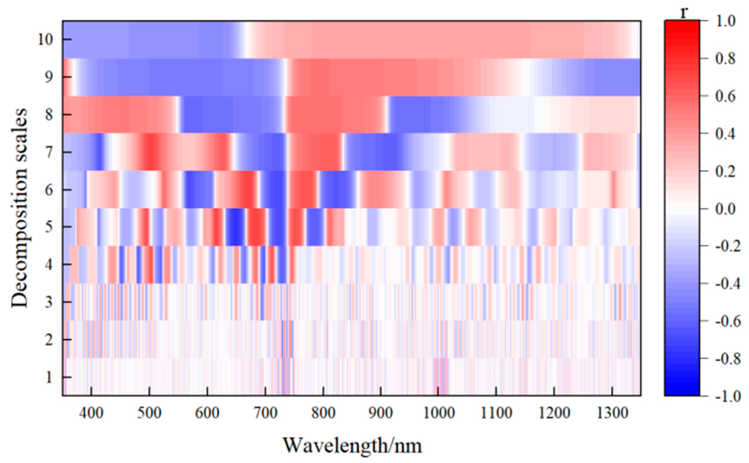
3.2. Correlation Analysis under Different Decomposition Scales Based on CWT

The spectral reflectance of winter wheat canopy is subjected to CWT processing by sym8 wavelet mother function to obtain wavelet energy coefficients. The correlation coefficient matrix diagrams of correlation coefficient and PNC under different decomposition scales are shown in Figure 2. In general, the correlation coefficient increases first, then decreases with the increase in the wavelet decomposition scale. The larger area is mainly concentrated in the 400–900 nm range of the visible and near-infrared regions, and the correlation coefficient is in the range of 900–1350 nm. The overall coefficient is low. In the low decomposition scale 1–3 areas, the correlation coefficient is relatively low and the overall change is not large and there are almost no areas with high correlation coefficients. In the region of medium decomposition scale 4–7, the decomposition scale with lower correlation coefficient is greatly improved and the correlation coefficient can reach 0.65, −0.77, 0.72 and 0.71 at the decomposition scale of 4–7, respectively, while at the high decomposition scale 8–10, the correlation coefficient is relatively evenly distributed and there is no particularly prominent correlation coefficient value. Therefore, the wavelet coefficient used to estimate winter wheat PNC in this study may be located in the 4–7 area of the medium decomposition scale.

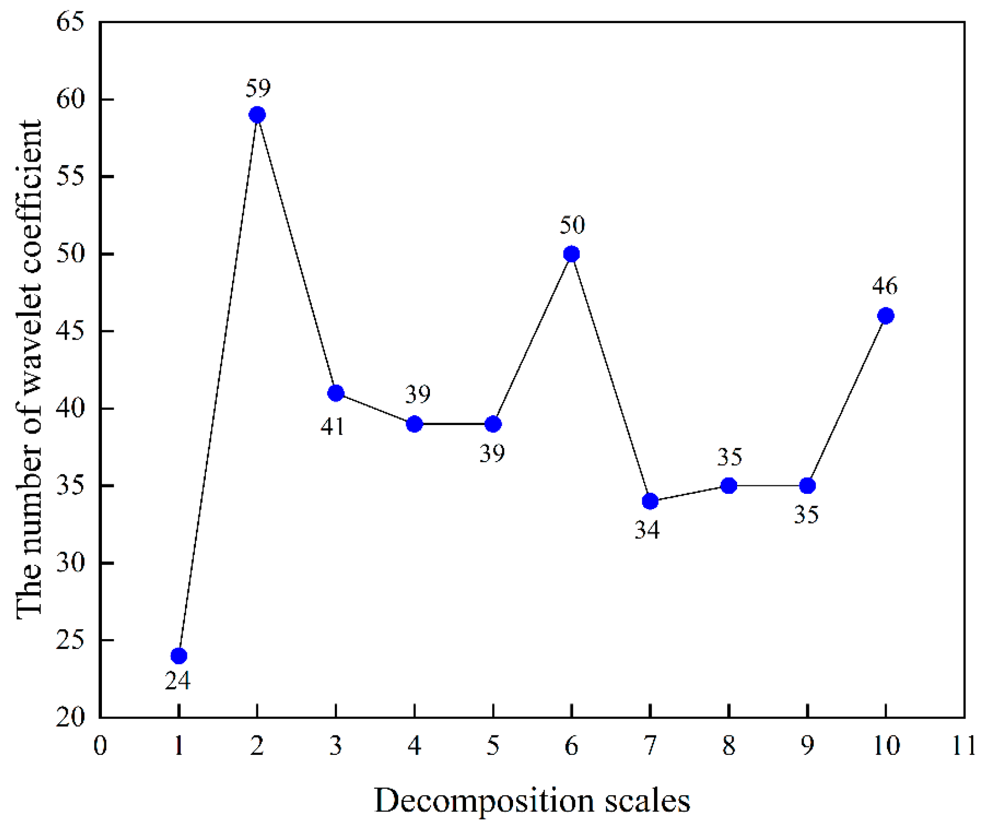
3.3. Screening of Wavelet Coefficient Based on SPA

In order to further eliminate the collinearity and data redundancy between wavelet coefficients based on CWT, obtaining a more promising winter wheat PNC prediction model, SPA was used to filter the variables. Figure 3 shows the number of the screening of wavelet coefficient by SPA based on different decomposition scales. Among them, CWT has relatively more wavelet coefficients at the second and sixth decomposition scales, 59 and 50, respectively, while the number of wavelets coefficient on decomposition scale 1 is the least; In sum, after the 1001 wavelet coefficients of each decomposition type were screened by SPA, all the number of wavelet coefficients has been significantly reduced.

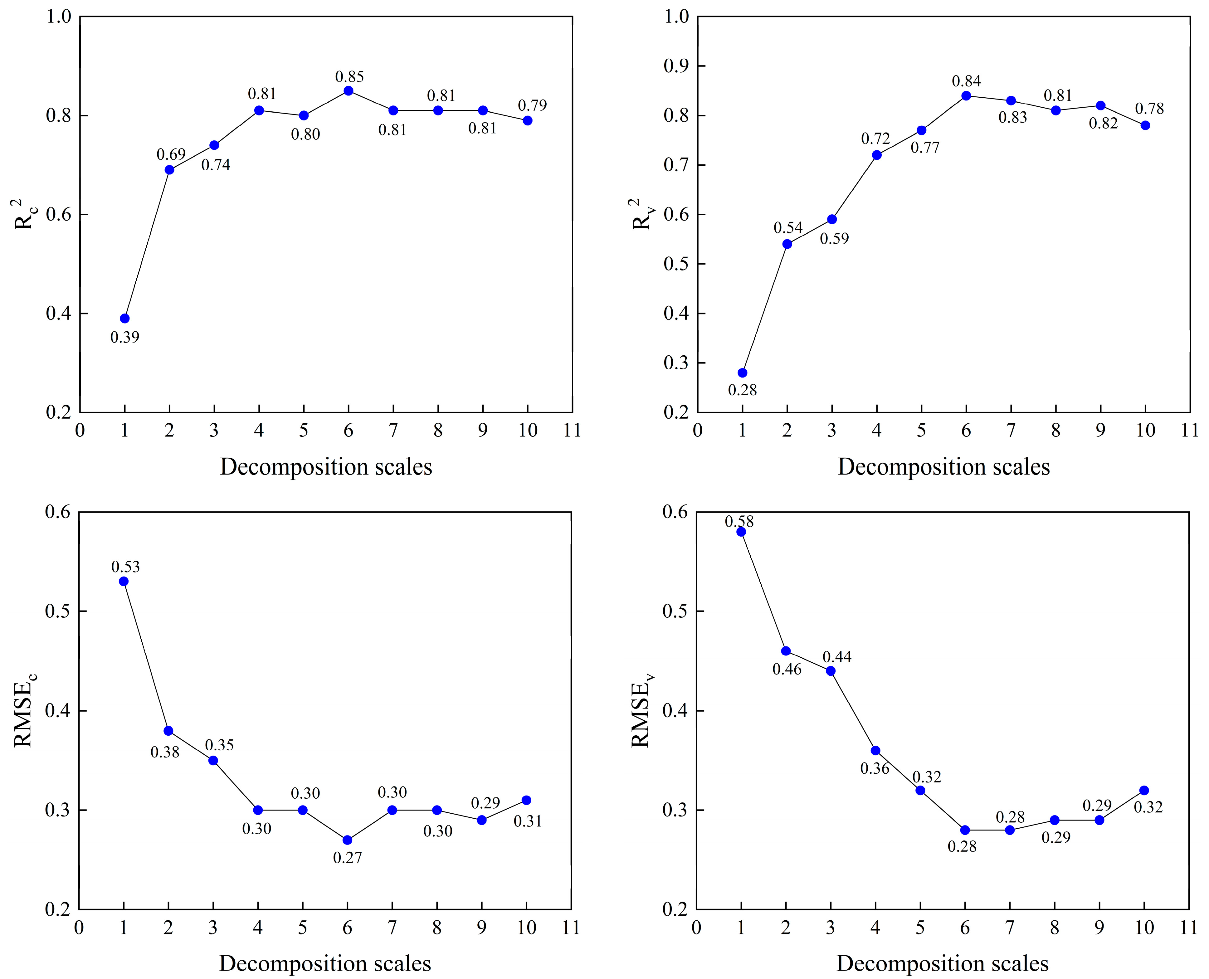
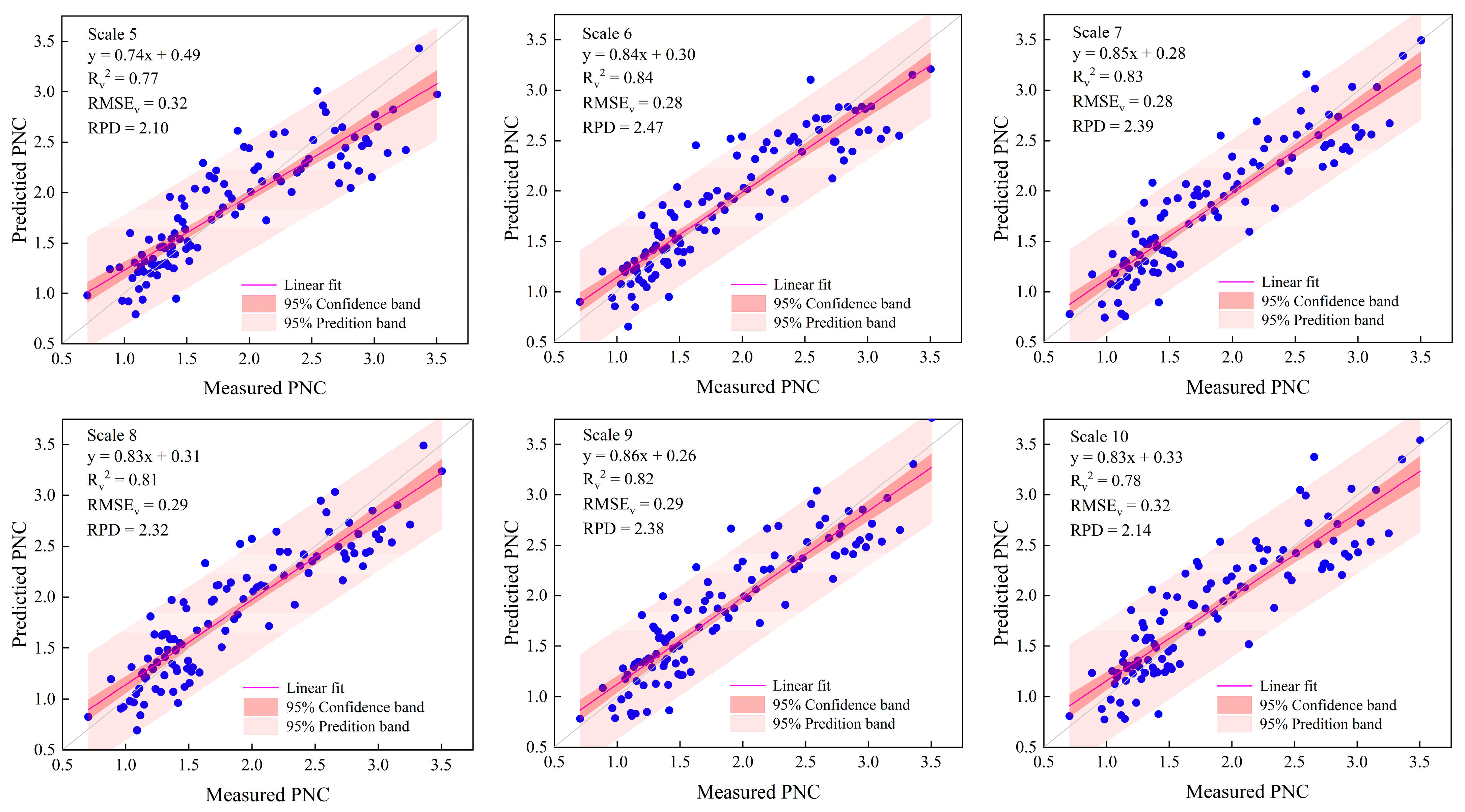
3.4. Estimation of Winter Wheat PNC Based on CWT-SPA-PLS

With various sensitive wavelet coefficients selected by SPA as input variables and winter wheat PNC as response variables, PLS regression models based on different decomposition scales for predicting PNC were constructed, respectively. The accuracy of calibration and validation set are shown in Figure 4. In general, the calibration and validation results of all prediction models have good prediction ability. In the calibration results, the Rc2 of all PNC prediction models increases first, then decreases with the increase in decomposition scale. On the contrary, the overall trend of RMSEc is to decrease first, then increase. Among all models, CWT–Scale6–SPA–PLS has the lowest Rc2 (0.39) and highest RMSEc (0.53). CWT–Scale6–SPA–PLS has the highest Rc2 (0.85) and lowest RMSEc (0.27), which has the strongest predictive ability. In the validation result, Rv2 and RMSEv in all PNC prediction models have similar trends in the corresponding calibration results of Rc2 and RMSEc. CWT–Scale6–SPA–PLS also gives the highest Rv2 (0.84) and the lowest RMSEv (0.28). The optimal winter wheat PNC prediction model is given by CWT–Scale6–SPA–PLS.

3.5. Model Accuracy Comparison

As shown in Figure 5, the RPD was used to further evaluate the model accuracy of winter wheat PNC. Compared with the prediction models of the lower decomposition scale (1–4), the RPD of the higher decomposition scale (5–10) models were greater than 2, indicating the models constructed by wavelet coefficient had excellent predictive ability based on the high decomposition scale. The prediction model of the lower decomposition scale (1–4) has a rough sample estimation ability (RPD < 1.4). Among them, the CWT–Scale6–SPA–PLS model had the highest accuracy, with an RPD to 2.47. The spatial distribution of PNC measured and predicted values of all models with RPD > 2 is shown in Figure 6. It can be seen that the fitting distribution of measured and predicted values of winter wheat PNC prediction model constructed by CWT–Scale6–SPA–PLS is closer to 1:1. The RPD of CWT–Scale6–SPA–PLS is the highest in all models, with Rc2, Rv2 as the highest and RMSEc, RMSEv as the lowest, indicating that the estimation model has excellent prediction ability.

4. Discussion

4.1. Analysis of Continuous Wavelet Transform (CWT)

As an efficient signal processing tool, CWT has been applied to quantitative analysis of crop parameters by more and more researchers [49,50,51]. This is mainly due to the fact that CWT can effectively eliminate the noise information attached to the spectral band while retaining the full band hyperspectral characteristics [30]. As shown in Figure 1, the wavelet coefficient increases with the increase in the decomposition scale, and the high−frequency noise gradually decreases. Properly increasing the decomposition scale can weaken the impact of high−frequency noise on the prediction model, which is conducive to highlighting the hyperspectral feature information, as shown in the scale 5–8 in Figure 1. The same conclusions have been drawn from previous studies [26,52]. However, when the decomposition scale is too large, the hyperspectral curve will become smooth, leading to the lack of certain feature information that is helpful for predictive analysis, such as scales 9 and 10 in Figure 1. When Liu et al. [35] used CWT to analyze potato chlorophyll content, the results showed the medium-scale wavelet decomposition can capture the information that can truly reflect potato chlorophyll content to a certain extent. As shown in Figure 2, the correlation coefficient matrix diagram of wavelet coefficient and PNC under different decomposition scales based on CWT indicated the correlation coefficient can reach 0.65, −0.77, 0.72 and 0.71 at the decomposition scale of 4–7, respectively, which is higher than the correlation coefficient in the region of high or low decomposition scales, illustrating both low and high CWT decomposition scales were not conducive to the reflection of crop absorption characteristics. Similar conclusions have been drawn in previous research [53,54,55].

4.2. Screening of Sensitive Wavelet Coefficient by SPA

Hyperspectral reflectance data has large information capacity and strong band continuity, but there are also problems, such as data redundancy and over fitting. Therefore, sensitive variable optimization is particularly important for quantitative estimation of winter wheat PNC. The commonly used sensitive variable screening method CARS has been widely used in previous studies and achieved good research result [35,56], but the process of CARS is complex and cumbersome. However, SPA can ensure the minimum collinearity between the selected characteristic bands, thus reducing the complexity of fitting in the process of model establishment and speeding up the fitting operation speed. In this study, SPA is used to screen the wavelet coefficients obtained by CWT. After SPA screening, all the number of wavelet coefficients has been significantly reduced as shown in Figure 3. The results show that SPA can remove the invalid information with large interference from the wavelet coefficients processed by CWT, while retaining the wavelet coefficients with the lowest information redundancy, thus producing satisfactory model prediction accuracy. Similar findings have also been found in previous studies [57]. However, some studies have shown that SPA has disadvantages, such as introducing some independent variables with low correlation with the target variable [58]. In future research, we need to develop a more satisfactory screening method of sensitive variables based on SPA theory as far as possible to meet the needs of quantitative estimation of crop parameters.

4.3. Accuracy Estimation of PNC Models

With various sensitive wavelet coefficients selected by SPA as input variables and winter wheat PNC as response variables, PLS regression models based on different decomposition scales for predicting PNC were constructed, respectively. The results showed CWT–Scale6–SPA–PLS based on wavelet coefficient of the sixth decomposition scale most accurately predicted the PNC (Rc2 = 0.85, RMSEc = 0.27, Rv2 = 0.84, RMSEv = 0.28) in Figure 4. In Figure 5, compared with the prediction model of the lower decomposition scale (1–4), the RPD of the higher decomposition scale (5–10) model was greater than 2, indicating the models constructed by wavelet coefficient had excellent predictive ability based on the high decomposition scale. The results indicated CWT–Scale6–SPA–PLS also is the optimal winter wheat PNC prediction model (RPD = 2.47). It could be seen that CWT–Scale6–SPA–PLS had good robustness and adaptability. Therefore, CWT–Scale6–SPA–PLS could be recommended as a basic model for winter wheat PNC estimation. The research results also show the feasibility and necessity of developing the combination of feature variable selection algorithm and PLS regression. Previous research also indicate that screening sensitive variables before PLS regression model can improve the low prediction accuracy and avoid over fitting, thus improving the accuracy of prediction model [38,59,60].

5. Conclusions

This study explored the feasibility of estimating winter wheat plant nitrogen concentration (PNC) by combining canopy hyperspectral reflectance, continuous wavelet transform (CWT), successive projections algorithm (SPA) and partial least squares (PLS) regression through three consecutive years of winter wheat field experiments. The results of this study showed the regions with large correlation coefficients between the wavelet coefficients obtained by CWT processing and PNC are basically located in the middle decomposition scale of 4–7. After SPA screening, all the number of wavelet coefficients has been significantly reduced. The PNC estimation model (CWT–Scale6–SPA–PLS) based on the wavelet coefficients of the sixth decomposition scale most accurately predicted the winter wheat PNC (Rc2 = 0.85, RMSEc = 0.27, Rv2 = 0.84, RMSEv = 0.28 and RPD = 2.47). This approach was reliable for PNC estimation and could be regarded as a basic model for the proposal of precise fertilizer management strategy for winter wheat. However, more variety tests are still needed in subsequent experiments to prove our research conclusions are still valid and more studies are needed to further compare different mother wavelets to improve the accuracy of nitrogen diagnosis in the management of precision nitrogen fertilizer.

Author Contributions

Conceptualization, X.C.; methodology, X.C.; software, X.C.; validation, X.C., Q.C. and F.L.; formal analysis, X.C.; investigation, X.C.; resources, Q.C.; data curation, X.C.; writing—original draft preparation, X.C.; writing—review and editing, X.C.; visualization, X.C.; supervision, Q.C. and F.L.; project administration, F.L.; funding acquisition, Q.C. All authors have read and agreed to the published version of the manuscript.

Funding

This research was funded by the National Natural Science Foundation of China (41701398).

Data Availability Statement

Data sharing is not application to this article.

Conflicts of Interest

The authors declare no conflict of interest.

References

  1. Yu, Z.; Wang, J.-w.; Chen, L.-p.; Fu, Y.-y.; Zhu, H.-c.; Feng, H.-k.; Xu, X.-g.; Li, Z.-h. An entirely new approach based on remote sensing data to calculate the nitrogen nutrition index of winter wheat. J. Integr. Agric. 2021, 20, 2535–2551. [Google Scholar]
  2. Huang, S.; Miao, Y.; Yuan, F.; Cao, Q.; Ye, H.; Lenz-Wiedemann, V.I.; Bareth, G. In-season diagnosis of rice nitrogen status using proximal fluorescence canopy sensor at different growth stages. Remote Sens. 2019, 11, 1847. [Google Scholar] [CrossRef]
  3. Li, F.; Wang, L.; Liu, J.; Wang, Y.; Chang, Q. Evaluation of leaf N concentration in winter wheat based on discrete wavelet transform analysis. Remote Sens. 2019, 11, 1331. [Google Scholar] [CrossRef]
  4. Liang, L.; Di, L.; Zhang, L.; Deng, M.; Qin, Z.; Zhao, S.; Lin, H. Estimation of crop LAI using hyperspectral vegetation indices and a hybrid inversion method. Remote Sens. Environ. 2015, 165, 123–134. [Google Scholar] [CrossRef]
  5. Wang, L.; Chang, Q.; Li, F.; Yan, L.; Huang, Y.; Wang, Q.; Luo, L. Effects of growth stage development on paddy rice leaf area index prediction models. Remote Sens. 2019, 11, 361. [Google Scholar] [CrossRef]
  6. Kiala, Z.; Odindi, J.; Mutanga, O.; Peerbhay, K. Comparison of partial least squares and support vector regressions for predicting leaf area index on a tropical grassland using hyperspectral data. J. Appl. Remote Sens. 2016, 10, 036015. [Google Scholar] [CrossRef]
  7. Yuan, H.; Yang, G.; Li, C.; Wang, Y.; Liu, J.; Yu, H.; Feng, H.; Xu, B.; Zhao, X.; Yang, X. Retrieving soybean leaf area index from unmanned aerial vehicle hyperspectral remote sensing: Analysis of RF, ANN, and SVM regression models. Remote Sens. 2017, 9, 309. [Google Scholar] [CrossRef]
  8. Sims, D.A.; Gamon, J.A. Relationships between leaf pigment content and spectral reflectance across a wide range of species, leaf structures and developmental stages. Remote Sens. Environ. 2002, 81, 337–354. [Google Scholar] [CrossRef]
  9. Wu, C.; Han, X.; Niu, Z.; Dong, J. An evaluation of EO-1 hyperspectral Hyperion data for chlorophyll content and leaf area index estimation. Int. J. Remote Sens. 2010, 31, 1079–1086. [Google Scholar] [CrossRef]
  10. Liang, L.; Qin, Z.; Zhao, S.; Di, L.; Zhang, C.; Deng, M.; Lin, H.; Zhang, L.; Wang, L.; Liu, Z. Estimating crop chlorophyll content with hyperspectral vegetation indices and the hybrid inversion method. Int. J. Remote Sens. 2016, 37, 2923–2949. [Google Scholar] [CrossRef]
  11. Xu, M.; Liu, R.; Chen, J.M.; Liu, Y.; Shang, R.; Ju, W.; Wu, C.; Huang, W. Retrieving leaf chlorophyll content using a matrix-based vegetation index combination approach. Remote Sens. Environ. 2019, 224, 60–73. [Google Scholar] [CrossRef]
  12. Zhang, J.; Tian, H.; Wang, D.; Li, H.; Mouazen, A.M. A novel approach for estimation of above-ground biomass of sugar beet based on wavelength selection and optimized support vector machine. Remote Sens. 2020, 12, 620. [Google Scholar] [CrossRef]
  13. Yue, J.; Zhou, C.; Guo, W.; Feng, H.; Xu, K. Estimation of winter-wheat above-ground biomass using the wavelet analysis of unmanned aerial vehicle-based digital images and hyperspectral crop canopy images. Int. J. Remote Sens. 2021, 42, 1602–1622. [Google Scholar] [CrossRef]
  14. Soltanian, M.; Naderi Khorasgani, M.; Tadayyon, A. Estimation of above-ground biomass of winter wheat (Triticum aestivum L.) using multiple linear regression, artificial neural network models remote sensing data. J. Crop Prod. 2020, 13, 179–196. [Google Scholar]
  15. Fageria, N.K. The Use of Nutrients in Crop Plants; CRC Press: Boca Raton, FL, USA, 2016. [Google Scholar]
  16. Kovács, P.; Vyn, T.J. Relationships between ear-leaf nutrient concentrations at silking and corn biomass and grain yields at maturity. Agron. J. 2017, 109, 2898–2906. [Google Scholar] [CrossRef]
  17. Gaju, O.; Allard, V.; Martre, P.; Le Gouis, J.; Moreau, D.; Bogard, M.; Hubbart, S.; Foulkes, M.J. Nitrogen partitioning and remobilization in relation to leaf senescence, grain yield and grain nitrogen concentration in wheat cultivars. Field Crops Res. 2014, 155, 213–223. [Google Scholar] [CrossRef]
  18. Li, F.; Miao, Y.; Hennig, S.D.; Gnyp, M.L.; Chen, X.; Jia, L.; Bareth, G. Evaluating hyperspectral vegetation indices for estimating nitrogen concentration of winter wheat at different growth stages. Precis. Agric. 2010, 11, 335–357. [Google Scholar] [CrossRef]
  19. Patel, M.K.; Ryu, D.; Western, A.W.; Suter, H.; Young, I.M. Which multispectral indices robustly measure canopy nitrogen across seasons: Lessons from an irrigated pasture crop. Comput. Electron. Agric. 2021, 182, 106000. [Google Scholar] [CrossRef]
  20. Dong, R.; Miao, Y.; Wang, X.; Chen, Z.; Yuan, F.; Zhang, W.; Li, H. Estimating plant nitrogen concentration of maize using a leaf fluorescence sensor across growth stages. Remote Sens. 2020, 12, 1139. [Google Scholar] [CrossRef]
  21. Yu, K.; Li, F.; Gnyp, M.L.; Miao, Y.; Bareth, G.; Chen, X. Remotely detecting canopy nitrogen concentration and uptake of paddy rice in the Northeast China Plain. ISPRS J. Photogramm. Remote Sens. 2013, 78, 102–115. [Google Scholar] [CrossRef]
  22. Chen, P.; Haboudane, D.; Tremblay, N.; Wang, J.; Vigneault, P.; Li, B. New spectral indicator assessing the efficiency of crop nitrogen treatment in corn and wheat. Remote Sens. Environ. 2010, 114, 1987–1997. [Google Scholar] [CrossRef]
  23. Stroppiana, D.; Boschetti, M.; Brivio, P.A.; Bocchi, S. Plant nitrogen concentration in paddy rice from field canopy hyperspectral radiometry. Field Crops Res. 2009, 111, 119–129. [Google Scholar] [CrossRef]
  24. Wang, L.; Chen, S.; Li, D.; Wang, C.; Jiang, H.; Zheng, Q.; Peng, Z. Estimation of paddy rice nitrogen content and accumulation both at leaf and plant levels from UAV hyperspectral imagery. Remote Sens. 2021, 13, 2956. [Google Scholar] [CrossRef]
  25. Yao, X.; Huang, Y.; Shang, G.; Zhou, C.; Cheng, T.; Tian, Y.; Cao, W.; Zhu, Y. Evaluation of six algorithms to monitor wheat leaf nitrogen concentration. Remote Sens. 2015, 7, 14939–14966. [Google Scholar] [CrossRef]
  26. Wang, H.-f.; Huo, Z.-g.; Zhou, G.-s.; Liao, Q.-h.; Feng, H.-k.; Wu, L. Estimating leaf SPAD values of freeze-damaged winter wheat using continuous wavelet analysis. Plant Physiol. Biochem. 2016, 98, 39–45. [Google Scholar] [CrossRef]
  27. Bruce, L.M.; Koger, C.H.; Li, J. Dimensionality reduction of hyperspectral data using discrete wavelet transform feature extraction. IEEE Trans. Geosci. Remote Sens. 2002, 40, 2331–2338. [Google Scholar] [CrossRef]
  28. Blackburn, G.A.; Ferwerda, J.G. Retrieval of chlorophyll concentration from leaf reflectance spectra using wavelet analysis. Remote Sens. Environ. 2008, 112, 1614–1632. [Google Scholar] [CrossRef]
  29. Chen, J.; Li, F.; Wang, R.; Fan, Y.; Raza, M.A.; Liu, Q.; Wang, Z.; Cheng, Y.; Wu, X.; Yang, F. Estimation of nitrogen and carbon content from soybean leaf reflectance spectra using wavelet analysis under shade stress. Comput. Electron. Agric. 2019, 156, 482–489. [Google Scholar] [CrossRef]
  30. Cheng, T.; Rivard, B.; Sanchez-Azofeifa, A. Spectroscopic determination of leaf water content using continuous wavelet analysis. Remote Sens. Environ. 2011, 115, 659–670. [Google Scholar] [CrossRef]
  31. Zhang, J.; Pu, R.; Loraamm, R.W.; Yang, G.; Wang, J. Comparison between wavelet spectral features and conventional spectral features in detecting yellow rust for winter wheat. Comput. Electron. Agric. 2014, 100, 79–87. [Google Scholar] [CrossRef]
  32. Liao, Q.; Wang, J.; Yang, G.; Zhang, D.; Lii, H.; Fu, Y.; Li, Z. Comparison of spectral indices and wavelet transform for estimating chlorophyll content of maize from hyperspectral reflectance. J. Appl. Remote Sens. 2013, 7, 073575. [Google Scholar] [CrossRef]
  33. Li, L.; Geng, S.; Lin, D.; Su, G.; Zhang, Y.; Chang, L.; Ji, Y.; Wang, Y.; Wang, L. Accurate modeling of vertical leaf nitrogen distribution in summer maize using in situ leaf spectroscopy via CWT and PLS-based approaches. Eur. J. Agron. 2022, 140, 126607. [Google Scholar] [CrossRef]
  34. Wang, Z.; Chen, J.; Zhang, J.; Tan, X.; Raza, M.A.; Ma, J.; Zhu, Y.; Yang, F.; Yang, W. Assessing canopy nitrogen and carbon content in maize by canopy spectral reflectance and uninformative variable elimination. Crop J. 2022, 30, 1224–1238. [Google Scholar] [CrossRef]
  35. Liu, N.; Xing, Z.; Zhao, R.; Qiao, L.; Li, M.; Liu, G.; Sun, H. Analysis of Chlorophyll Concentration in Potato Crop by Coupling Continuous Wavelet Transform and Spectral Variable Optimization. Remote Sens. 2020, 12, 2826. [Google Scholar] [CrossRef]
  36. Bangalore, A.S.; Shaffer, R.E.; Small, G.W.; Arnold, M.A. Genetic algorithm-based method for selecting wavelengths and model size for use with partial least-squares regression: Application to near-infrared spectroscopy. Anal. Chem. 1996, 68, 4200–4212. [Google Scholar] [CrossRef] [PubMed]
  37. Galvao, R.K.H.; Araujo, M.C.U.; Fragoso, W.D.; Silva, E.C.; Jose, G.E.; Soares, S.F.C.; Paiva, H.M. A variable elimination method to improve the parsimony of MLR models using the successive projections algorithm. Chemom. Intell. Lab. Syst. 2008, 92, 83–91. [Google Scholar] [CrossRef]
  38. Li, H.; Liang, Y.; Xu, Q.; Cao, D. Key wavelengths screening using competitive adaptive reweighted sampling method for multivariate calibration. Anal. Chim. Acta 2009, 648, 77–84. [Google Scholar] [CrossRef]
  39. Fan, L.; Zhao, J.; Xu, X.; Liang, D.; Yang, G.; Feng, H.; Yang, H.; Wang, Y.; Chen, G.; Wei, P. Hyperspectral-based estimation of leaf nitrogen content in corn using optimal selection of multiple spectral variables. Sensors 2019, 19, 2898. [Google Scholar] [CrossRef]
  40. Bai, L.-m.; Li, F.-l.; Chang, Q.-r.; Zeng, F.; Cao, J.; Lu, G. Increasing accuracy of hyper · spectral remote sensing for total nitrogen of winter wheat canopy by use of SPA and PLS methods. J. Plant. Nutr. Fertil. 2018, 24, 52–58. [Google Scholar]
  41. Ollinger, S.V. Sources of variability in canopy reflectance and the convergent properties of plants. New Phytol. 2011, 189, 375–394. [Google Scholar] [CrossRef]
  42. Luo, J.; Ying, K.; He, P.; Bai, J. Properties of Savitzky–Golay digital differentiators. Digit. Signal Process. 2005, 15, 122–136. [Google Scholar] [CrossRef]
  43. Liao, Q.; Gu, X.; Li, C.; Chen, L.; Huang, W.; Du, S.; Fu, Y.; Wang, J. Estimation of fluvo-aquic soil organic matter content from hyperspectral reflectance based on continuous wavelet transformation. Trans. Chin. Soc. Agric. Eng. 2012, 28, 132–139. [Google Scholar]
  44. Araújo, M.C.U.; Saldanha, T.C.B.; Galvao, R.K.H.; Yoneyama, T.; Chame, H.C.; Visani, V. The successive projections algorithm for variable selection in spectroscopic multicomponent analysis. Chemom. Intell. Lab. Syst. 2001, 57, 65–73. [Google Scholar] [CrossRef]
  45. Wold, S.; Sjöström, M.; Eriksson, L. PLS-regression: A basic tool of chemometrics. Chemom. Intell. Lab. Syst. 2001, 58, 109–130. [Google Scholar] [CrossRef]
  46. Nigon, T.J.; Yang, C.; Dias Paiao, G.; Mulla, D.J.; Knight, J.F.; Fernández, F.G. Prediction of Early Season Nitrogen Uptake in Maize Using High-Resolution Aerial Hyperspectral Imagery. Remote Sens. 2020, 12, 1234. [Google Scholar] [CrossRef]
  47. Chauchard, F.; Cogdill, R.; Roussel, S.; Roger, J.; Bellon-Maurel, V. Application of LS-SVM to non-linear phenomena in NIR spectroscopy: Development of a robust and portable sensor for acidity prediction in grapes. Chemom. Intell. Lab. Syst. 2004, 71, 141–150. [Google Scholar] [CrossRef]
  48. Singh, K.P.; Malik, A.; Basant, N.; Saxena, P. Multi-way partial least squares modeling of water quality data. Anal. Chim. Acta 2007, 584, 385–396. [Google Scholar] [CrossRef]
  49. Li, C.; Wang, Y.; Ma, C.; Ding, F.; Li, Y.; Chen, W.; Li, J.; Xiao, Z. Hyperspectral estimation of winter wheat leaf area index based on continuous wavelet transform and fractional order differentiation. Sensors 2021, 21, 8497. [Google Scholar] [CrossRef]
  50. Zhao, R.; An, L.; Song, D.; Li, M.; Qiao, L.; Liu, N.; Sun, H. Detection of chlorophyll fluorescence parameters of potato leaves based on continuous wavelet transform and spectral analysis. Spectrochim. Acta Part A Mol. Biomol. Spectrosc. 2021, 259, 119768. [Google Scholar] [CrossRef]
  51. Yao, Q.; Zhang, Z.; Lv, X.; Chen, X.; Ma, L.; Sun, C. Estimation Model of Potassium Content in Cotton Leaves Based on Wavelet Decomposition Spectra and Image Combination Features. Front. Plant Sci. 2022, 13, 920532. [Google Scholar] [CrossRef]
  52. Wang, Z.; Chen, J.; Fan, Y.; Cheng, Y.; Wu, X.; Zhang, J.; Wang, B.; Wang, X.; Yong, T.; Liu, W. Evaluating photosynthetic pigment contents of maize using UVE-PLS based on continuous wavelet transform. Comput. Electron. Agric. 2020, 169, 105160. [Google Scholar] [CrossRef]
  53. Li, D.; Wang, X.; Zheng, H.; Zhou, K.; Yao, X.; Tian, Y.; Zhu, Y.; Cao, W.; Cheng, T. Estimation of area-and mass-based leaf nitrogen contents of wheat and rice crops from water-removed spectra using continuous wavelet analysis. Plant Methods 2018, 14, 1–20. [Google Scholar] [CrossRef] [PubMed]
  54. Li, D.; Cheng, T.; Jia, M.; Zhou, K.; Lu, N.; Yao, X.; Tian, Y.; Zhu, Y.; Cao, W. PROCWT: Coupling PROSPECT with continuous wavelet transform to improve the retrieval of foliar chemistry from leaf bidirectional reflectance spectra. Remote Sens. Environ. 2018, 206, 1–14. [Google Scholar] [CrossRef]
  55. Li, Y.; Via, B.K.; Li, Y. Lifting wavelet transform for Vis-NIR spectral data optimization to predict wood density. Spectrochim. Acta Part A Mol. Biomol. Spectrosc. 2020, 240, 118566. [Google Scholar] [CrossRef]
  56. Yang, B.; Wang, M.; Sha, Z.; Wang, B.; Chen, J.; Yao, X.; Cheng, T.; Cao, W.; Zhu, Y. Evaluation of Aboveground Nitrogen Content of Winter Wheat Using Digital Imagery of Unmanned Aerial Vehicles. Sensors 2019, 19, 4416. [Google Scholar] [CrossRef] [PubMed]
  57. Chen, X.; Lv, X.; Ma, L.; Chen, A.; Zhang, Q.; Zhang, Z. Optimization and Validation of Hyperspectral Estimation Capability of Cotton Leaf Nitrogen Based on SPA and RF. Remote Sens. 2022, 14, 5201. [Google Scholar] [CrossRef]
  58. Li, Z.; Tang, X.; Shen, Z.; Yang, K.; Zhao, L.; Li, Y. Comprehensive comparison of multiple quantitative near-infrared spectroscopy models for Aspergillus flavus contamination detection in peanut. J. Sci. Food Agric. 2019, 99, 5671–5679. [Google Scholar] [CrossRef]
  59. Devos, O.; Duponchel, L. Parallel genetic algorithm co-optimization of spectral pre-processing and wavelength selection for PLS regression. Chemom. Intell. Lab. Syst. 2011, 107, 50–58. [Google Scholar] [CrossRef]
  60. Jiang, H.; Zhang, H.; Chen, Q.; Mei, C.; Liu, G. Identification of solid state fermentation degree with FT-NIR spectroscopy: Comparison of wavelength variable selection methods of CARS and SCARS. Spectrochim. Acta Part A Mol. Biomol. Spectrosc. 2015, 149, 1–7. [Google Scholar] [CrossRef]
Figure 1. Curves of wavelet coefficient at different decomposition scales based on CWT.
Remotesensing 15 00997 g001
Figure 2. Correlation coefficient matrix diagram of wavelet coefficient and PNC under different decomposition scales based on CWT.
Remotesensing 15 00997 g002
Figure 3. The number of the screening of wavelet coefficient by SPA based on different decomposition scales.
Remotesensing 15 00997 g003
Figure 4. Rc2, RMSEc, Rv2 and RMSEv of PNC estimation models.
Remotesensing 15 00997 g004
Figure 5. Comparison of RPD values of PNC estimation models based on different decomposition scales.
Remotesensing 15 00997 g005
Figure 6. Spatial distribution of PNC measured values and predicted values of all models with RPD > 2. The 1:1 line was represented by the gray line.
Remotesensing 15 00997 g006
Table 1. Summary of the details in the three wheat growth experiments.
Exp.Sowing TimeSampling and Sensing Date
2016
QianOct. 2ndMarch 26 (GS3), April 14 (GS5), April 28 (GS6), May 17 (GS7), May 26 (GS8). (2017)
2017
QianOct. 2ndMarch 29 (GS3), April 18 (GS5), May 7 (GS7), May 22 (GS8). (2018)
2018
QianOct. 1stMarch 31 (GS3), April 20 (GS5), April 29 (GS6), May 17 (GS7). (2019)
Note: Qian represent Qian County. GS3: stem elongation, GS5: heading, GS6: flowering, GS7: development of fruit, GS8: ripening.
Table 2. Statistical description of winter wheat PNC (%) in the whole growth period.
Data SetsNumber of SamplesMaximumMinimumAverageSDCV (%)
All5403.690.591.860.6836.56
Calibration4323.690.591.860.6836.56
Validation1083.500.701.880.6836.17
Disclaimer/Publisher’s Note: The statements, opinions and data contained in all publications are solely those of the individual author(s) and contributor(s) and not of MDPI and/or the editor(s). MDPI and/or the editor(s) disclaim responsibility for any injury to people or property resulting from any ideas, methods, instructions or products referred to in the content.

