Article

An Intercomparison of Sentinel-1 Based Change Detection Algorithms for Flood Mapping

by
Mark Edwin Tupas
1,2,*,
Florian Roth
1,
Bernhard Bauer-Marschallinger
1 and
Wolfgang Wagner
1
1
Remote Sensing Research Group, Department of Geodesy and Geoinformation, TU Wien, 1040 Vienna, Austria
2
Department of Geodetic Engineering, University of the Philippines, Quezon City 1101, Philippines
*
Author to whom correspondence should be addressed.
Remote Sens. 2023, 15(5), 1200; https://doi.org/10.3390/rs15051200
Submission received: 16 December 2022 / Revised: 15 February 2023 / Accepted: 16 February 2023 / Published: 22 February 2023
(This article belongs to the Special Issue Remote Sensing of Climate-Related Hazards)

Abstract

:
With its unrivaled and global land monitoring capability, the Sentinel-1 mission has been established as a prime provider in SAR-based flood mapping. Compared to suitable single-image flood algorithms, change-detection methods offer better robustness, retrieving flood extent from a classification of observed changes. This requires data-based parametrization. Moreover, in the scope of global and automatic flood services, the employed algorithms should not rely on locally optimized parameters, which cannot be automatically estimated and have spatially varying quality, impacting much on the mapping accuracy. Within the recently launched Global Flood Monitoring (GFM) service, we implemented a Bayes-Inference (BI)-based algorithm designed to meet these ends. However, whether other change detection algorithms perform similarly or better is unknown. This study examines four Sentinel-1 change detection models: The Normalized Difference Scattering Index (NDSI), Shannon’s entropy of NDSI (SNDSI), Standardized Residuals (SR), and Bayes Inference over Luzon in the Philippines, which was flood-hit by a typhoon in November 2020. After parametrization assessment against an expert-created Sentinel-1 flood map, the four models are inter-compared against an independent Sentinel-2 classification. The obtained findings indicate that the Bayes change detection profits from its scalable classification rules and shows the least sensitivity to parametrization choices while also performing best in terms of mapping accuracy. For all change detection models, a backscatter seasonality model for the no-flood reference delivered best results.

Graphical Abstract

1. Introduction

Flooding is a significant concern all over the world. In global disaster assessment reports, it consistently ranks among the most destructive of natural disasters. Unfortunately, flood frequency and severity are expected to increase for most of the world due to climate change [1], with further increased human exposure due to population growth. Therefore, rapid assessments of flood extent and impacts using Earth observation satellites are of great importance. Due to their capacity to capture high-resolution images of the Earth’s surface even in stormy weather, Synthetic Aperture Radar (SAR) sensors are unrivaled in their capability to map large-scale flooding. Hence, most disaster mapping services, such as the Copernicus Emergency Management Service (CEMS) [2], and the Sentinel Asia initiative [3] utilize SAR satellites for their operations. In the past, these services have delivered SAR-based flood maps only upon requests from affected areas, manually operated by human experts. This implies that flood events may be missed in the case of late or non-activation. To avoid this and improve timeliness, CEMS has recently launched a Global Flood Monitoring (GFM) service that analyses Sentinel-1 SAR data in a fully automatic fashion [4].
In principle, mapping flood extent from SAR images is relatively straightforward given that backscatter from open water bodies is normally relatively low compared to backscatter from the surrounding land surface areas. Thus, when mapping flooded areas from individual SAR images on demand, SAR image analysts usually work with simple thresholding techniques. However, selecting a threshold value that works everywhere under all weather conditions is clearly impossible [5,6]. Therefore, in the fully automatic GFM service, a relatively simple problem turns into the significant scientific challenge of finding a robust flood detection model that works globally without the need for manual fine-tuning of its parameters.
A large variety of methods to map flood extent from SAR imagery has already been published, including change detection-based approaches [7,8], split-window or tiled thresholding techniques [5,9,10,11], Bayesian [12,13,14,15,16] and machine learning methods [17,18,19]. Most studies yielded excellent results for specific test areas, but the performance on a large scale is often not known [20]. Moreover, while reviews and assessments of these SAR flood and inundation mapping methods are available [21,22,23], it has been pointed out that direct performance comparisons are limited [24]. However, such comparisons are crucial in designing and improving operational systems that perform at large scales, e.g., regional or global extents. Last but not least, distinct parameterizations might be required for these methods to perform at the same level in different areas. Thus, the robustness of parameterization is a crucial indicator when selecting flood mapping workflows for implementation at scale [25,26,27]. Unfortunately, this aspect usually is not treated explicitly in the scientific literature so far.
For the design of robust flood detection models and their parameterization, it is highly advantageous to work with SAR backscatter data cubes that allow efficient access to the data not just in the spatial but also temporal dimension [28,29]. Using the Sentinel-1 backscatter data cube built up at the Earth Observation Data Centre (EODC) [30], it has, e.g., been possible to parameterize a Bayesian flood detection model at the level of individual pixels by analyzing backscatter time series for each pixel [27]. Another example is the Sentinel-1 data cube implementation at the Google Earth Engine [31], which already hosts several waterbody and flood mapping workflows [32,33].
In this contribution, we compare the performance of four change detection models for mapping floods using Sentinel-1 SAR data (Section 2). Compared to approaches that map floods only based on single SAR images, the parameterization of change detection models is normally less problematic, allowing to apply them over large and diverse domains. Nonetheless, even the parameterization of change detection models may involve a lot of choices that can have a strong impact on the accuracy of the derived flood maps, in particular, the choices of the no-flood reference image and the threshold for labeling an SAR pixel as flooded. Hence, in our study, we investigated how sensitive the different model are to changes in their parameterization.
As a study case, we chose a flood event that occurred in the Cagayan river basin in the Northern Philippines in November 2020. This choice was motivated by the fact that the area, which is situated in the Pacific typhoon belt, is projected to be significantly impacted by climate change, including a general rise in precipitation with an indication of higher frequency of heavy rainfall events [34] and, consequently, a greater threat of flooding [35]. The study region and data are described in Section 3. The methods for intercomparing the four change detection models and assessing the robustness of their parameterizations are introduced in Section 4, followed by the presentation of the results on parametrization and model-intercomparison in Section 5 and Section 6. Finally, Section 7 contains the discussion and conclusions.

2. Change Detection Algorithms

Change detection approaches for flood mapping compare in one way or another an SAR backscatter image potentially containing flood pixels with a reference SAR scene describing a non-flooded situation. By comparing two images, spatial signal variations are reduced, simplifying the task of finding suitable thresholds and model parameterizations that work for different land cover classes. Furthermore, the use of a no-flood reference image allows for excluding other low backscatter areas that tend to be mislabeled as a flood. Nonetheless, factors such as speckle and overall high variability of the backscatter measurements prompt the need for some additional means of normalization. This problem is solved differently in the four change detection models that we selected for this study, namely the Normalized Scattering Difference Index, the Shannon’s entropy of NDSI, the Standardized Residuals, and a Bayesian Inference method. Given that the choice of the no-flood reference and different thresholding techniques has an important impact on the performance of these four models, these parameterizations are discussed separately in Section 2.5 and Section 2.6.

2.1. Normalized Difference Scattering Index

Indices such as the Normalized Difference Scattering Index (NDSI) [36] and the Normalized Difference Ratio [37], while differently named, are similarly computed from backscatter data from a flood image and a no-flood reference. For our purposes, we adopt the NDSI for the rest of the document and compute it with:
NDSI = σ 0 σ r 0 σ 0 + σ r 0
where σ 0 represents the SAR image pixels that are potentially flooded and σ r 0 the no-flood reference. Both σ 0 and σ r 0 are expressed in m 2 m 2 . In this formulation, flooded areas are associated with large negative numbers due to the decrease in backscatter when the land surface is inundated, i.e., a pixel is labeled as flooded when NDSI is smaller than a chosen threshold value. The normalization term σ 0 + σ r 0 helps to reduce the impact of signal variations in the reference image.

2.2. Shannon’s Entropy of NDSI

Ulloa et al. [36] extends the NDSI concept further by computing the Shannon’s entropy of NDSI using a 9 × 9 moving window. The premise of this approach is that flooded pixels are often adjacent to other flooded pixels (save for boundaries) and, thus, should primarily have a smooth texture. Furthermore, since entropy measures the level of uncertainty of possible grayscale values in a given area, it also serves as a textural measure. Shannon’s entropy of NDSI, referred to here as SNDSI, is computed by:
SNDSI = n p log 2 p
where p is the probability of NDSI estimated from a normalized histogram count for all n pixels in the moving window. As for the NDSI, pixels are classified as flooded when SNDSI becomes smaller than a chosen threshold.

2.3. Standardized Residuals

An alternative approach to normalize the difference term σ 0 σ r 0 is to use a measure of variance of the backscatter measurements [7,8,32,38]. Here, we adopt the terminology of Schlaffer et al. [7] who computed Standardized Residuals (SR)
SR = σ 0 σ r 0 S t D e v ( σ 0 )
where S t D e v ( σ 0 ) is the temporal standard deviation of σ 0 for non-flooded conditions. S t D e v ( σ 0 ) is computed from historic σ 0 time series for each pixel describing the variability of the backscatter measurements due to changes in soil moisture, vegetation, or other environmental factors for each location. Thereby, a pixel is considered to be flooded if SR has a large negative value which indicates that σ 0 is outside the expected signal range. Note that because of the need to compute S t D e v ( σ 0 ) from historic time series, the SR model is substantially more input-data-demanding than the NDSI and SNDSI models that can in principle be run with just two input images. Nonetheless, similar to NDSI and SNDSI, one needs to chose a threshold.

2.4. Bayesian Inference

Instead of normalizing differences, another method of comparing flood and no-flood situations is to use probabilistic approaches. The method adopted here is based on a pixel-based Bayesian Inference (BI) method [16,27] that considers the temporal SAR backscatter information of a non-flooded pixel to estimate its non-flooded conditional probability distribution, p ( σ 0 | N ) . The conditional flooded probability distribution, p ( σ 0 | F ) , can be estimated from geographically distributed calm open water samples. The probability that a σ 0 measurement over one pixel indicates flood conditions is calculated with [13,14,16]:
BI p ( F | σ 0 ) = p ( σ 0 | F ) p ( F ) p ( σ 0 | F ) p ( F ) + p ( σ 0 | N ) p ( N )
where p ( F ) and p ( N ) are the prior probabilities of a pixel being flooded and non-flooded (in short simply “priors”). Here, we adopt non-informed priors, with both p ( F ) and p ( N ) assumed to have equal, i.e., 0.5, prior probability. A pixel is labeled as a flood if the flood probability p ( F | σ 0 ) is greater than 0.5. For ease of discussion, we refer to the numerical value of p ( F | σ 0 ) as BI in the following sections. Note that in contrast to the other three models, the final decision criterion is well defined, i.e., BI > 0.5. Like SR, the BI model is input-data demanding, requiring a backscatter data cube to pre-compute p ( σ 0 | N ) per pixel.

2.5. Thresholding Techniques

Except for the BI method, the change detection models introduced above require the choice of a threshold to label an SAR pixel as flooded or non-flooded. The choices one can make range from choosing one fixed threshold value for all SAR images and the entire study domain to threshold values computed for each SAR image individually or even subsets of a SAR image. Similar to the work of Landyut et al. [24], we test fixed threshold values taken from the literature and thresholds dynamically selected using histogram-based methods. In particular, we investigate the performance of global Otsu’s [39] and Kittler and Illingworth’s (KI) methods [40] along with best performing fixed value from the source materials.

2.6. Selection of No-Flood Reference

In principle, the selection of the no-flood reference σ r 0 has a great effect on all models described above. When choosing a real SAR image as reference, one would like to choose a scene that resembles—except for the inundation areas—the unflooded conditions as good as possible in terms of land cover and environmental conditions. This may, e.g., be the latest pre-flood image or a SAR image acquired in the same season the previous year. While automated methods for the selection of such real reference images have been proposed [20,41], the computation of synthetic no-flood reference is a viable alternative approach when working with SAR backscatter data cube. Here, we test the generation of synthetic σ r 0 images by computing the mean backscatter and the expected seasonal backscatter value for the day of year [7]. Median, as used by Clement’s work [8] was left out in the analysis due to its similarity with the mean estimate for this study site.

3. Data and Study Site

3.1. Sentinel-1 Data Cube

The analysis was performed on a Sentinel-1 SAR backscatter data cube that includes all imagery acquired over the study region from January 2018 to December 2020. The data cube was generated with a dedicated pre-processing engine that ingests Sentinel-1A/B Ground Range Detected (GRD) products, as outlined in detail in Wagner et al. [30]. The pre-processing workflow includes (1) application of precise orbit file, (2) border noise removal, (3) thermal noise reduction, (4) radiometric calibration, (5) range-doppler terrain correction, and (6) resampling and reprojection to the Equi7Grid tiling system [42]. The data cube was abstracted from these hierarchically organized Sentinel-1 images using the yeoda package developed by TU Wien [43]. The backscatter data cube was filtered for VV polarization and Sentinel-1’S relative orbit, to obtain all images from the same observation geometry.

3.2. Study Area

The study area is situated on Luzon, the largest and most populous island of the Philippines. The study area extent is defined by the 100 × 100 km-sized tile “E058N117T1” from the Equi7Grid tiling system, shown as the red footprint in Figure 1. The area covers a part of the Cagayan valley, where vast tracks of agricultural fields are situated. The Cagayan River traverses the tile from south to north. Urban settlements can mostly be found near the river, while most of the western portion of the tile is dominated by mountainous terrain. All subsequent analysis in this work were performed at 10 × 10 m resolution native to this data cube tile. Collected data sets were rasterized, if needed, and reprojected to the Equi7Grid tile.
The flooding event investigated in this study was caused by typhoon Vamco that hit the northern Philippines from 9 to 13 November 2020. The typhoon affected more than five million individuals [44], and many along the Cagayan River were flood-stricken. The flood scene for the analysis was captured by Sentinel-1B on the ascending orbit 069 on 13 November 2020 around the time of peak flooding.

3.3. Reference Flood Maps

Due to the fleeting nature of floods ground truth is often lacking [45]. This is also the case here, but two satellite-based reference flood maps are available. The first is a flood map (in shapefile format) generated from the same Sentinel-1 flood scene from 13 November 2020 by experts working at the Sentinel Asia [3] who were well familiar with the study area and the flooding caused by the typhoon Vamco (Sentinel Asia Typhoon Vamco Activation—https://sentinel-asia.org/EO/2020/article20201111PH.html, accessed on 12 December 2022). From personal communication with the operators, we know that the Sentinel Asia product was created from the SAR intensity difference, whereas the threshold was manually selected and optimized. However, it should be noted that the experts at Sentinel Asia also did not have access to ground observations.
We generated a second reference flood map, using a pair of optical multispectral images from Sentinel-2 (Table 1), one acquired two months before (on 9 September 2020) and one during the flood event (on 13 November 2020). Specifically, we used Level2A (Bottom of Atmosphere) images downloaded from the Copernicus Open Access Hub and processed them using Sentinel-2 toolbox of SNAP v8.0 [46], applying thick clouds and cirrus cloud mask. Then we computed the Modified Normalized Difference Water Index (MNDWI) that was designed to delineate water and built-up areas [47]. The flood extent was finally derived by comparing the two MNDWI images and fine-tuning the threshold. Due to the significant cloud cover on 13 November 2020, only a portion of the flood scene could be mapped. Fortunately, the main channel of the Cagayan River is cloud-free and offers sufficient samples. While the Sentinel-2 acquisition took place 7 h after Sentinel-1, no major appreciable differences in the flood extent are visible (See Figure 2).

3.4. Auxiliary Data

The workflows implemented in this work require auxiliary information on topography and geomorphology. In this study, we used the Height Above Nearest Drainange (HAND) Index [48] and the Projected Local Incidence Angle (PLIA) as shown in Figure 3. The HAND index data was derived from the Copernicus Digital Elevation Model (CopDEM GLO-30—https://doi.org/10.5270/ESA-c5d3d65, accessed on 9 November 2022) upsampled to the resolution of the working tile. The PLIA map was generated as a by-product of the Sentinel-1 pre-processing workflow and is thus stored in the same tile’s projection system. The applicability of these auxiliary data—HAND and PLIA are discussed in the following section.

4. Methods

To compare the performance of the four change detection models and their sensitivity to changes in their parameterization, we follow a two step approach: In the first step, we assess for each change detection model separately how different parameterizations impact the results. As we are only interested in the relative performance of the parameterizations when applying the models to Sentinel-1 data, the benchmark in this step is the Sentinel-1 flood map produced by the experts of Sentinel Asia. In the second step, we intercompare the performance of the four change detection models with their best-performing parameterizations by assessing their accuracy against the Sentinel-2 flood map.
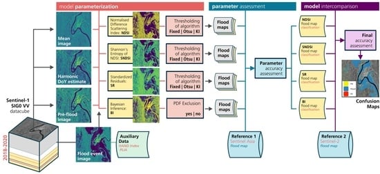
The detailed workflow is shown in Figure 4. The starting point is the Sentinel-1 backscatter data cube from which all required VV backscatter images from relative orbit 69 and the corresponding projected local incidence angle (PLIA) are extracted. Furthermore, a common set of geomorphological and exclusion masking post-processing steps are applied to all flood maps. First, the Height Above Nearest Drainage (HAND) index is used to mask for terrain distortions in the SAR data, such as radar shadow and layover [49] at a height above 20 m (in this case) from drainage. Second, a PLIA mask is applied to remove pixels which have PLIA outside the typical range of incidence angles for flat areas (where floods are typically appearing), following the approach by [27]. These masks helped to reduce the number of falsely classified flood pixels over the mountainous parts of the study area—which are generally troubling SAR retrievals—thereby slightly improving the accuracy of the flood maps. Lastly, 5 × 5 spatial majority filters are applied as a morphological correction of salt-and-pepper-like classification coming from SAR signal components unrelated to flood conditions.

4.1. Paramterizations

To test the NDSI, SNDSI, and SR models —and their parameterizations—we computed a multitude of flood maps using different combinations of the no-flood reference and the thresholding technique to parameterize the models. Here, we show the results for the combination of three no-flood references and three different thresholds, yielding in total 3 × 3 × 3 = 27 flood maps. With respect to the no-flood reference, the three used parameterizations are:
  • Mean Backscatter: We computed the mean and standard deviation of σ 0 per pixel over the three year long data record (2018–2020). Note that while the NDSI and SNDSI only require the mean as input, the SR requires both the mean and S t D e v ( σ 0 ) .
  • Harmonic Model: To account for seasonal signal variations, we fitted a harmonic model to the data record, yielding for each pixel and each day of year (DOY) an estimate of the expected backscatter intensity and its standard deviation, respectively. For a detailed description of this Harmonic model formulation we refer the readers to the recent work of Bauer-Marschallinger et al. [27].
  • Pre-flood Image: A Sentinel-1 image acquired about two weeks before the flood event on 1 November 2020 and from the same relative orbit was selected as no-flood reference of the backscatter intensity. As the SR and BI models also require an estimate of the backscatter dynamics, we compute S t D e v ( σ 0 ) , similar to harmonic formulation, using the Root Mean of Square of the difference between backscatter in the time-series data record and the expected no-flood backscatter (from pre-flood image).
The three models NDSI, SNDSI, and SR require a threshold for label pixels as either flood or no-flood. In the course of finding an optimal threshold, we apply the simple pre-filtering technique applied by Schlaffer et al. [7] using the HAND index, where the pixels of high HAND values, i.e., HAND > 20, are removed from the histogram before thresholds are determined.
We tested three different methods to determine the threshold:
  • Fixed: Here, we rely on published reports. Among the NDSI and SNDSI implementations, thresholds from the work of Ulloa et al. [36] were adopted. These are −0.725 for NDSI and 0.78 for SNDSI. While for SR a fixed value of −1.5 was found by several studies to provide good results [8].
  • Otsu: In the method of Otsu [39], an assumption of bi-modality is followed by fitting two distributions by minimizing intra-class intensity variance. Hence, we determine the threshold from the intersection of the fitted distributions within our reference- and flood-images.
  • Kittler and Illingsworth (KI): As an alternative we also tested the KI method [40]. Also known as the Minimum-Error thresholding method, it seeks to fit the two distributions, using the minimum error criterion, to a given model histogram. Hence, the threshold is similarly determined from the intersection of the fitted distributions as with Otsu above.
To test the BI model, we employ the same three no-flood reference parameterizations to derive the full conditional probability function p ( σ 0 | N ) . While BI does not rely on parameterized thresholds, we test the application (and non-application) of distribution-based masking methods introduced in the previous work of Bauer-Maschallinger et al. [27]. Accordingly, the BI method is improved by excluding pixels with high classification uncertainty, either from very similar a priori distributions for flood and no-flood, or from actual observation values that fall in-between the two. Consequently, the significant Probability Density Function (PDF) overlap between flooded and non-flooded classes, and in this paper, we refer to this as PDF exclusion mask. Hence, for BI we test 1 × 3 × 2 = 6 parameterizations, and finally obtain a set of 33 flood maps for our experiment.

4.2. Accuracy Assessment

The flood maps are evaluated by comparing them to the two reference flood maps described in Section 3.3. Given that these two expert-produced reference maps also do not represent an absolute “truth”, the computed accuracy metrics must be interpreted with some caution. Nonetheless, as we are mostly interested in understanding the relative performances of the algorithms and their parameterizations, they represent a good benchmark.
We computed traditional land cover classification metrics: Overall Accuracy (OA), Producer’s Accuracy (PA), and User’s Accuracy (UA). OA was selected over chance agreement corrected metric, i.e., Kappa coefficient, from recommendation in the literature [50,51]. In addition, we calculate the Critical Success Index (CSI), which is often used in data science and flood mapping work to address the inequality of the classes. CSI has been specifically found to provide good insights for flood mapping accuracy assessments at the same scale [24]. All of these metrics were computed from a binary confusion matrix and its four elements: True Positive (TP), True Negative (TN), False Positive (FP), and False Negative (FN), among classified pixels, according to the following formulas:
O A = T P + T N T P + T N + F P + F N
U A = T P ( T P + F P )
P A = T P ( T P + F N )
C S I = T P ( T P + F P + F N )
Following good practice examples and sampling size determination equations from Foody’s work [52], we acquired a total of 5000 random samples. Independent random samples per change detection model were taken to remove possible bias in the application of model-dependent exclusion masks. From this, we surmise that a difference greater than 2% in OA implies a consequential distinction between the results.

5. Model Parameter Assessment

In this section, we analyze the sensitivity of the four change detection models to changes in their parameterization by comparing the derived flood maps to the Sentinel-1 reference flood map produced by Sentinel Asia (Section 5.1, Section 5.2, Section 5.3 and Section 5.4). Furthermore, we select the best performing parameterizations for each method to be subject of our model inter-comparison in Section 6.
To allow a well-founded interpretation of the performance of the four models, we first examine their statistical bases used for the distinction between flood and no flood. Figure 5 shows the histograms and maps of the observed backscatter σ 0 together with the calculated NDSI, SNDSI, SR, and BI with, as an example, the mean image as no-flood reference. From this compilation, it can be observed that the histograms of the model values allow in most cases an improved distinction between flooded and non-flooded sections, compared with the initial flooded σ 0 image. Generally, the decrease in backscatter during floods is highlighted, and the change detection models show—as expected—increased image contrast and more distributed histograms. The SR map (Figure 5m–p), however, appears to highlight different signatures within the observed σ 0 image while not transforming the shape of the histogram. Another observation is that particularly the SR and BI data manage to register the pattern from the permanent water surfaces along the river, thus supporting the delineation against flood bodies.
For the whole area, NDSI (Figure 5e–h) provides the most considerable increase in the relative spread of values. The SNDSI (Figure 5i–l) shows less improvement in this regard, but reduces the spatial dispersion of these values compared with NDSI, which structurally features a noise-like spatial pattern (see e.g., in Figure 5h). Meanwhile, SR shows the least gain in contrast, and we would argue that there is no significant effect on the separability of the classes in its histogram (see in Figure 5m). This is most apparent in permanent low backscatter areas, such as the river pixels, that are not as well delineated as for the other methods (see in Figure 5p).
Concerning the threshold parameters (indicated by colored lines in the histograms of Figure 5), speciffically for SR and σ 0 , we observe that the respective Otsu and KI thresholds follow the same characteristics described by [24]. The results show more liberal flood labeling for Otsu’s method and more conservative labeling using KI. Meanwhile, the NDSI and SNDSI indicate significant variance and instability when it comes to finding the respective thresholds. This could be attributed to the seemingly non-Gaussian distributions of the non-flood class and flood class (as observed in Figure 5e,i), noting that these thresholding algorithms assume Gaussian distributions.
In the BI model data (Figure 5q–t), most of the visually perceived flooded areas were successfully assigned with high flood probability. Overall, the Bayes probability values show intriguing results, as the river pixels show a low flood probability in spite of the locally significant distribution overlaps coming from the river/water signature. While this is a positive result, this behavior could easily swing from non-flooded and flooded classes, as seen in the salt and pepper appearance of probability values along the river (see in Figure 5t). This similar noise-like appearance is also apparent in the probability values found in agricultural areas.

5.1. Parameterization of NDSI Model

We now examine the NDSI model and the performance of its different parameterizations. As shown in Table 2, the harmonic approach performs best of the no-flood references, while KI performs best of the threshold methods. Consequently, the combination of these two (represented by parameterization no. 6) builds the favored parametrization. This combination features a CSI value larger than 85%. One can observe the significant variance in the UA, ranging from moderate (59%) to excellent performance (97%). In contrast, the PA has smaller differences, with most showing excellent results above 90%. This suggests that the models favor, in general, overestimation. Thus, KI thresholding is a proper method to dampen this effect. One can also notice the erratic performance of the tested thresholding methods for the NDSI model. We attribute this to the fact that the NDSI histogram does not form a Gaussian distribution, a precondition leading to previous findings as e.g., by [36].

5.2. SNDSI Parameterization

Similar to NDSI, the harmonic no-flood reference leads to the best performance (see Table 3), followed by the pre-flood and the mean reference. The best-performing parameterization combines the harmonic reference and KI thresholding method. However, Otsu’s method appears to be the most stable among the thresholding methods, probably due to the fact that SNDSI shows no propensity towards overestimation as the NDSI does. Moreover, using Shannon’s entropy appears to be an effective spatial morphological filter to reduce noise-like classification.

5.3. Standardized Residuals Parameterization

In general, aside from UA, SR shows a similar large variance in accuracy metrics of the parameterizations (see Table 4). Concerning no-flood reference parameterization, also here, the harmonic outperforms mean and pre-flood references. The pre-flood reference does not perform well for this method because of the larger standard deviations in the temporal model for the three-year period we tested. The fixed S R = 1.5 threshold shows the best performance for this model in this study site. It shows a slightly better performance compared to Otsu’s method, while KI underperforms in this model. Overall, the model leans towards improving UA rather than PA values. The reported propensity towards underestimation by KI’s method is apparent for the SR model, as indicated by the lower PA results.

5.4. Bayes Inference Parameterization

In the case of the BI method, no threshold needs to be found, and the general rule of labeling is based on higher probability, i.e., >50.0%. Instead, Table 5 includes the PDF exclusion (see Section 5) as an option. One can see that there are minimal variations in the accuracy metrics for the BI method compared to the other change detection methods. The BI consistently performed very well in terms of UA; almost no non-flooded pixels are labeled as a flood and slightly lower PA indicates minor underestimation. Furthermore, all parametrizations reached a high CSI larger than 80%. Overall, the best-performing parameterization No. 4 uses the harmonic no-flood reference and the PDF-based exclusion masks from the Bayes model.
Based on the nominal values of OA and CSI, the BI method using harmonic reference slightly outperforms the other no-flood references. It should be noted that these differences are too marginal to conclude a significant distinction. Unlike in other methods, the pre-flood image performs similarly well as the mean and harmonic no-flood reference. It is also noticeable that the introduction of PDF exclusion masking consistently improves the BI model, albeit by small margins in CSI and OA. This, however, comes at the cost of masking some areas that could not be reliably classified.

5.5. Parameterization Summary

Table 6 collects the best-performing parameterization for each change detection model. All four models perform best with the harmonic model for the no-flood reference. The mean and pre-flood no-flood references performed variably depending on the other parameters. Concerning threshold method, KI’s method performed the best for NDSI and SNDSI. Despite KI’s method being found to be more conservative in thresholding [24], it performs best for certain instances due to improved separability of flood and non-flood pixels in the models (see histograms in Figure 5). For the SR model; however, the fixed threshold was found to provide consistently good results for this study site, while KI and Otsu depend on the no-flood reference. While Otsu’s method is not present within the collection of best-performing parameterizations, it shows less variance in performance compared to KI. This result is consistent with reports of Otsu’s performance [24]; here, significant flooding is apparent in the study site. Thus, its propensity to overestimate floods is not as pronounced. Lastly, the application PDF Exclusion step consistently improves the accuracy metrics for BI, albeit by only small percentage points.
After comparing different parameterizations for each change detection method, we infer the robustness of the methods for this study site given by the variability of the resulting accuracy metrics. The highest robustness is shown by the BI method. We suspect that the use of statistical distributions instead of a particular threshold is responsible for the superior robustness.

6. Model Intercomparison

The optimal parameterizations for each of the four change detection methods are identified in Section 5 and are summarized in Table 6. These are considered in the subsequent step, where the accuracy assessment metrics are computed against the Sentinel-2 flood map (see Table 7).
After parameter optimization, there are generally few false positive pixels in the SAR-based flood maps, as all selected flood maps show User’s Accuracy (UA) values greater than 87%. The Bayes method used has the highest value of 95.9%. As expected, the PA of all methods is significantly lower than UA. The PA results range from SNDSI with 77.0% to SR with 69.8%. Based on our assumption that there is no significant difference in the flood extent due to little time lag between the Sentinel-1 observation and the Sentinel-2-based reference map, this result can be attributed to the limitation of SAR-based methods over certain land cover types. As reported already by Bauer-Marschallinger et al. [27], the SAR-based flood mapping is challenged in densely vegetated and urban areas, where optical systems such as Sentinel-2 can detect floods under good circumstances and in the absence of clouds.
The OA results indicate good or excellent general agreement between the tested flood maps and the reference maps, which is also promoted by the overall large area and the relatively large flooding event. Among the selected parameterizations, the Bayes method shows the highest OA value with 85.3%, while the last-ranked method SR has only a difference of 3.5%. Based on the little differences in OA, it can be said that BI has the only noteworthy difference from the other methods tested based on 2% difference criteria we established in Section 4.2. When examining the Critical Success Index (CSI) results, the Bayes method is also ranked best with 72.3%, followed by the SNDSI with 69.5%, NDSI with 68.2%, and SR with the lowest result at 65.7%. Only the BI method has CSI greater than 70.0%, while all others are rated closely. However, in reflection of the underlying differences in flood mapping mechanisms between optical and SAR-based maps, we consider all methods to perform well.
It should be noted that the above statistical metrics show a generalized performance description for the whole scene. Therefore, we have a closer look at the qualitative differences for some selected areas. PA and UA relate to classification pixels of false negatives (omission errors) and false positives (commission errors), which describe (dis-) agreement well when zoomed in on particular areas of interest. Figure 6 and Figure 7 show representative subsets and their confusion maps between the tested model’s flood maps and the Sentinel-2 reference map. These maps highlight the area near the city of Tuguegarao with its meandering river channel and surrounding agricultural areas, respectively.
The four methods successfully remove non-water areas of permanent low backscatter, such as the Cagayan airport shown in the upper right edge of the maps in Figure 6, fully exploiting the strength of the change detection concept. Moreover, the BI method shows an excellent delineation of the permanent river courses, being excluded in the flood result through the PDF exclusion approach. The SR method shows suitable results for permanent water exclusion but could be improved by further morphological operators as only small patches are observed. The NDSI-based results, show poor performance in this regard.
In contrast to the other models, SNDSI shows larger patches of false positives over the built-up areas in the center and east of the zoom-in (Figure 6). In this area, high backscatter from double bounce effects are clustered, which results in low entropy values that lead to erroneous labeling. The observed improvement in the NDSI and SNDSI in parameter transformation for thresholding does not significantly improve these methods compared to the other tested methods. This degraded performance could be attributed to the limitation of the parameter formulation to account for false positives, which are clearly seen in the confusion maps. For example, low SNDSI values mainly refer to swaths of water in an image, but are also likely for radar shadows which may have been missed by the post-processing masks. Another observation is the NDSI, and SNDSI results have more overestimation in flooded agricultural areas (Figure 7), while the SR and BI methods are less prone to this type of commission error.
As also seen in Table 7, SR has notably more false negatives. These are generally observed in agricultural areas, as exemplified in Figure 7, and can be attributed to the higher temporal variance from agricultural activities (in the historical time series), which dampens the SR parameter. Surprisingly, the BI method performs better than the other methods, considering that agricultural areas were recognized in need of improvement for the BI method presented by [27].
In terms of spatial cohesion of the flood maps, as inferred from the confusion maps in Figure 6 and Figure 7, the SNDSI and BI method show more cohesive overall results. For the area of Tuguegarao, Figure 6, the NDSI map shows noisy or patchy results in terms of higher rates of both FP and FN, while SR has the same concern to a lesser degree in the specific regions. At the same time, Figure 7 show much noise in all methods, including the BI result illustrating the challenges of such areas in flood mapping. It could be argued that NDSI and SR methods could further be improved with better morphological filtering during a post-processing step. Alternatively, by use of Shannon’s entropy as in the SNDSI, a filter-like improvement is achieved, which slightly improves the overall result for this case study.
However, notable in the BI result in Figure 7 are the patches of excluded areas. While in most cases, these coincide with misclassifications in the other maps, thus highlighting the PDF exclusion’s effectiveness. For example, some areas such as the old river meander in the lower left corner of the BI map in Figure 6 were excluded rather than labeled being as flood. Despite this and other things considered, the BI method generally performs better than the other methods tested in this study.

7. Conclusions

This study tested and compared four automated SAR-based change detection flood mapping methods and their parameterization against Sentinel-1-based expert data for the case study in the northern Philippines. Our parameterization experiments comprise the testing of different threshold and masking options, as well as the suitability of three different methods to generate the no-flood-reference map, which is crucial to any change detection approach. We further carried out an inter-comparison of the four best-performing model parameterizations, with accuracy assessment against a Sentinel-2-based flood map specifically generated for this study.
In our assessment of the model parameterizations against the semi-manual results from Sentinel Asia (using Sentinel-1), the Bayes Inference (BI) method showed the most consistent performance, regardless of the input no-flood reference. The BI model was found to be robust in the sense that it does not require tailor-fitting, whereas the other change detection methods were found to be more significantly impacted by one’s choice of input non-flood reference and the thresholding method. Focusing on the latter, Otsu’s method was found to work well with the SR and SNDSI methods. In contrast, KI’s method showed a better result for NDSI and SNDSI, albeit showing highly variable results when the input no-flood reference is changed. The published threshold of S R 1.5 also showed a good result for this study area. Lastly, considering that we applied a HAND-based prefiltering before thresholding and the obtained variability of the results, it is recommended to explore spatial prefiltering techniques with these models, which are driven by temporal parameters.
Concerning the no-flood-reference parameterization, the harmonic model lead to the best results for all four change detection models, apparently profiting from the good fit of the seasonally expected backscatter. The missing consideration of the backscatter’s seasonal variability causes the lower performance of the mean. The pre-flood image is generally observed close to the flood event and hence is expected to represent actual conditions such as vegetation state or soil moisture most accurately. Nevertheless, results from the pre-flood-parameterized models are less consistent compared to the harmonic model. We found that the pre-flood image—as an actual single-time observation—still holds speckle that leads to noise-like classifications, which is effectively removed in no-flood references made from temporal aggregations. Therefore, we recommended that the datacube-derived no-flood reference are further investigated, such as other time-series models, e.g., exponential filters, or parameter tuning through, e.g., modulating the length of the contributing time-series.
The evaluation of the best-performing model parameterizations against the optical-derived Sentinel-2 reference showed that the BI method performed best. Considering the parameterization results and this final comparison suggest that the BI core concept is generally more robust and possibly more adaptable to other study sites. Albeit computationally more demanding, the BI approach of taking the sample’s full distribution into account proves to be more adaptive than the discrete thresholding in the other methods.
All tested datacube flood mapping methods show meaningful agreement with the reference flood maps from Sentinel-2 and a semi-automatic expert product by Sentinel Asia. The best-performing methods all achieved good to excellent results based on OA and CSI. The four tested change detection methods show very satisfying User’s Accuracies, mainly through a correct classification of permanent low backscatter areas. The Producer’s Accuracies, on the other hand, also had reasonable performance but exhibit well-known SAR-related deficiencies over challenging land covers.
To summarize, this study represents one of the first efforts to inter-compare several SAR change-detection-based flood mapping methods and their parameterizations, with a view on the feasibility of applying them in an operational fashion over large areas. Overall, all four change detection models performed reasonably well considering that their input parameters were neither locally optimized nor adapted by a human operator. Nonetheless, the sensitivity of the NSDI, SNSRI, and SR models to parameterizations suggests the need for further localized tests. On the other hand, the Bayesian Inference model coupled with the harmonic model as no-flood reference seems to be relatively stable in its performance, which is an important prerequisite for (global) automatic operations.

Author Contributions

Conceptualization M.E.T. and W.W.; methodology M.E.T. and W.W.; software M.E.T. and F.R.; validation M.E.T. and F.R.; formal analysis M.E.T.; investigation F.R., M.E.T. and B.B.-M.; data curation M.E.T.; writing—original draft preparation M.E.T.; writing—review and editing ALL; visualization M.E.T. and B.B.-M.; supervision B.B.-M. and W.W. All authors have read and agreed to the published version of the manuscript.

Funding

This research work was performed with support of the Engineering Research & Development for Technology Program of the Philippine Department of Science and Technology, the project “S1Floods.AT” (Grant no. BW000028378) founded by the Austrian Rsearch Promotion Agency (FFG) and the project “Provision of an Automated, Global, Satellite-based Flood Monitoring Product for the Copernicus Emergency Management Service” (GFM), Contract No. 939866-IPR-2020 for the European Commission’s Joint Research Centre (EC-JRC). The authors acknowledge TU Wien Bibliothek for financial support through its Open Access Funding by TU Wien.

Data Availability Statement

The data presented in this study are openly available at: https://github.com/marxt/dc-flood-mapping-comp-ph (accessed on 11 January 2023).

Acknowledgments

The computational results presented have been achieved using inter alia the Vienna Scientific Cluster (VSC). We would further like to thank our colleagues at TU Wien and EODC for supporting us on technical tasks on maintaining the datacube. Special thanks is given to Chathumal Madhuranga of the Geoinformatic Center-Aisan Institute of Technology (GIC-AIT) for his valuable insights on the Sentinel Asia flood products. GIC-AIT acts as a Primary Data Analyzing node for Sentinel Asia.

Conflicts of Interest

The authors declare no conflict of interest.

Abbreviations

The following abbreviations are used in this manuscript:
CEMSCopernics Emergency Management Service
CSICritical Success Index
DEMDigital Elevation Model
DOYDay Of Year
EODCEarth Observation Data Centre for Water Resources Monitoring
GRDHGround Range Detected High-resolution SAR product
GFMGlobal Flood Monitoring
HANDHeight Above Nearest Drainage
IWInterferometric Wide Swath mode of Sentinel-1
OAOverall Accuracy
PAProducer Accuracy
PLIAProjected Local Incidence Angle θ
UAUser Accuracy
PDFProbability Distribution Function
MNDWIModified Normalized Difference Water Index
NDWINormalised Difference Water Index
NDSINormalised Difference Scattering Index
NRTNear-Real-Time
OAOverall Accuracy
SASentinel Asia
SARSynthetic Aperture Radar
SSESum of Squared Errors
SIG0Sigma Nought backscatter coefficient σ 0
SNDSIShanon’s entropy of Normalised Difference Scattering Index
SRStandardized Residuals

References

  1. Hirabayashi, Y.; Mahendran, R.; Koirala, S.; Konoshima, L.; Yamazaki, D.; Watanabe, S.; Kim, H.; Kanae, S. Global flood risk under climate change. Nat. Clim. Change 2013, 3, 816–821. [Google Scholar] [CrossRef]
  2. Wania, A.; Joubert-Boitat, I.; Dottori, F.; Kalas, M.; Salamon, P. Increasing Timeliness of Satellite-Based Flood Mapping Using Early Warning Systems in the Copernicus Emergency Management Service. Remote Sens. 2021, 13, 2114. [Google Scholar] [CrossRef]
  3. Kaku, K. Satellite remote sensing for disaster management support: A holistic and staged approach based on case studies in Sentinel Asia. Int. J. Disaster Risk Reduct. 2019, 33, 417–432. [Google Scholar] [CrossRef]
  4. Salamon, P.; Mctlormick, N.; Reimer, C.; Clarke, T.; Bauer-Marschallinger, B.; Wagner, W.; Martinis, S.; Chow, C.; Böhnke, C.; Matgen, P.; et al. The New, Systematic Global Flood Monitoring Product of the Copernicus Emergency Management Service. In Proceedings of the 2021 IEEE International Geoscience and Remote Sensing Symposium IGARSS, Brussels, Belgium, 11–16 July 2021; pp. 1053–1056. [Google Scholar] [CrossRef]
  5. Martinis, S.; Twele, A.; Voigt, S. Towards operational near real-time flood detection using a split-based automatic thresholding procedure on high resolution TerraSAR-X data. Nat. Hazards Earth Syst. Sci. 2009, 9, 303–314. [Google Scholar] [CrossRef]
  6. Giustarini, L.; Hostache, R.; Matgen, P.; Schumann, G.J.P.; Bates, P.D.; Mason, D.C. A Change Detection Approach to Flood Mapping in Urban Areas Using TerraSAR-X. IEEE Trans. Geosci. Remote Sens. 2013, 51, 2417–2430. [Google Scholar] [CrossRef] [Green Version]
  7. Schlaffer, S.; Matgen, P.; Hollaus, M.; Wagner, W. Flood detection from multi-temporal SAR data using harmonic analysis and change detection. Int. J. Appl. Earth Obs. Geoinf. 2015, 38, 15–24. [Google Scholar] [CrossRef]
  8. Clement, M.A.; Kilsby, C.G.; Moore, P. Multi-temporal synthetic aperture radar flood mapping using change detection. J. Flood Risk Manag. 2018, 11, 152–168. Available online: https://onlinelibrary.wiley.com/doi/pdf/10.1111/jfr3.12303 (accessed on 9 April 2022). [CrossRef] [Green Version]
  9. Twele, A.; Cao, W.; Plank, S.; Martinis, S. Sentinel-1-based flood mapping: A fully automated processing chain. Int. J. Remote Sens. 2016, 37, 2990–3004. [Google Scholar] [CrossRef]
  10. Bioresita, F.; Puissant, A.; Stumpf, A.; Malet, J.P. A method for automatic and rapid mapping of water surfaces from Sentinel-1 imagery. Remote Sens. 2018, 10, 217. [Google Scholar] [CrossRef] [Green Version]
  11. Liang, J.; Liu, D. A local thresholding approach to flood water delineation using Sentinel-1 SAR imagery. ISPRS J. Photogramm. Remote Sens. 2020, 159, 53–62. [Google Scholar] [CrossRef]
  12. Westerhoff, R.S.; Kleuskens, M.P.H.; Winsemius, H.C.; Huizinga, H.J.; Brakenridge, G.R.; Bishop, C. Automated global water mapping based on wide-swath orbital synthetic-aperture radar. Hydrol. Earth Syst. Sci. 2013, 17, 651–663. [Google Scholar] [CrossRef] [Green Version]
  13. Refice, A.; Capolongo, D.; Pasquariello, G.; D’Addabbo, A.; Bovenga, F.; Nutricato, R.; Lovergine, F.P.; Pietranera, L. SAR and InSAR for Flood Monitoring: Examples With COSMO-SkyMed Data. IEEE J. Sel. Top. Appl. Earth Obs. Remote Sens. 2014, 7, 2711–2722. [Google Scholar] [CrossRef]
  14. Giustarini, L.; Hostache, R.; Kavetski, D.; Chini, M.; Corato, G.; Schlaffer, S.; Matgen, P. Probabilistic Flood Mapping Using Synthetic Aperture Radar Data. IEEE Trans. Geosci. Remote Sens. 2016, 54, 6958–6969. [Google Scholar] [CrossRef]
  15. D’Addabbo, A.; Refice, A.; Pasquariello, G.; Lovergine, F.P.; Capolongo, D.; Manfreda, S. A Bayesian Network for Flood Detection Combining SAR Imagery and Ancillary Data. IEEE Trans. Geosci. Remote Sens. 2016, 54, 3612–3625. [Google Scholar] [CrossRef]
  16. Schlaffer, S.; Chini, M.; Giustarini, L.; Matgen, P. Probabilistic mapping of flood-induced backscatter changes in SAR time series. Int. J. Appl. Earth Obs. Geoinf. 2017, 56, 77–87. [Google Scholar] [CrossRef]
  17. De la Cruz, R.M.; Olfindo, N.T., Jr.; Felicen, M.M.; Borlongan, N.J.B.; Difuntorum, J.K.L.; Marciano, J.J.S., Jr. Near-Realtime Flood Detection From Multi-Temporal Sentinel Radar Images Using Artificial Intelligence. Int. Arch. Photogramm. Remote Sens. Spat. Inf. Sci. 2020, XLIII-B3-2020, 1663–1670. [Google Scholar] [CrossRef]
  18. Mayer, T.; Poortinga, A.; Bhandari, B.; Nicolau, A.P.; Markert, K.; Thwal, N.S.; Markert, A.; Haag, A.; Kilbride, J.; Chishtie, F.; et al. Deep learning approach for Sentinel-1 surface water mapping leveraging Google Earth Engine. ISPRS Open J. Photogramm. Remote Sens. 2021, 2, 100005. [Google Scholar] [CrossRef]
  19. Zhao, J.; Li, Y.; Matgen, P.; Pelich, R.; Hostache, R.; Wagner, W.; Chini, M. Urban-Aware U-Net for Large-Scale Urban Flood Mapping Using Multitemporal Sentinel-1 Intensity and Interferometric Coherence. IEEE Trans. Geosci. Remote Sens. 2022, 60, 1–21. [Google Scholar] [CrossRef]
  20. Zhao, J.; Chini, M.; Matgen, P.; Hostache, R.; Pelich, R.; Wagner, W. An Automatic SAR-Based Change Detection Method for Generating Large-Scale Flood Data Records: The UK as a Test Case. In Proceedings of the IGARSS 2019—2019 IEEE International Geoscience and Remote Sensing Symposium, Yokohama, Japan, 28 July–2 August 2019; pp. 6138–6141. [Google Scholar] [CrossRef]
  21. Schumann, G.J.P.; Moller, D.K. Microwave remote sensing of flood inundation. Phys. Chem. Earth Parts A/B/C 2015, 83-84, 84–95. [Google Scholar] [CrossRef]
  22. Martinis, S.; Kuenzer, C.; Wendleder, A.; Huth, J.; Twele, A.; Roth, A.; Dech, S. Comparing four operational SAR-based water and flood detection approaches. Int. J. Remote Sens. 2015, 36, 3519–3543. [Google Scholar] [CrossRef]
  23. Shen, X.; Wang, D.; Mao, K.; Anagnostou, E.; Hong, Y. Inundation extent mapping by synthetic aperture radar: A review. Remote Sens. 2019, 11, 879. [Google Scholar] [CrossRef] [Green Version]
  24. Landuyt, L.; Wesemael, A.V.; Schumann, G.J.; Hostache, R.; Verhoest, N.E.C.; Coillie, F.M.B.V. Flood Mapping Based on Synthetic Aperture Radar: An Assessment of Established Approaches. IEEE Trans. Geosci. Remote Sens. 2019, 57, 722–739. [Google Scholar] [CrossRef]
  25. Martinis, S.; Kersten, J.; Twele, A. A fully automated TerraSAR-X based flood service. ISPRS J. Photogramm. Remote Sens. 2015, 104, 203–212. [Google Scholar] [CrossRef]
  26. Chini, M.; Hostache, R.; Giustarini, L.; Matgen, P. A Hierarchical Split-Based Approach for Parametric Thresholding of SAR Images: Flood Inundation as a Test Case. IEEE Trans. Geosci. Remote Sens. 2017, 55, 6975–6988. [Google Scholar] [CrossRef]
  27. Bauer-Marschallinger, B.; Cao, S.; Tupas, M.E.; Roth, F.; Navacchi, C.; Melzer, T.; Freeman, V.; Wagner, W. Satellite-Based Flood Mapping through Bayesian Inference from a Sentinel-1 SAR Datacube. Remote Sens. 2022, 14, 3673. [Google Scholar] [CrossRef]
  28. Ticehurst, C.; Zhou, Z.S.; Lehmann, E.; Yuan, F.; Thankappan, M.; Rosenqvist, A.; Lewis, B.; Paget, M. Building a SAR-Enabled Data Cube Capability in Australia Using SAR Analysis Ready Data. Data 2019, 4, 100. [Google Scholar] [CrossRef] [Green Version]
  29. Misev, D.; Baumann, P.; Bellos, D.; Wiehle, S. BigDataCube: A Scalable, Federated Service Platform for Copernicus. In Proceedings of the 2019 IEEE International Conference on Big Data (Big Data), Los Angeles, CA, USA, 9–12 December 2019; pp. 4103–4112. [Google Scholar] [CrossRef]
  30. Wagner, W.; Bauer-Marschallinger, B.; Navacchi, C.; Reuß, F.; Cao, S.; Reimer, C.; Schramm, M.; Briese, C. A Sentinel-1 Backscatter Datacube for Global Land Monitoring Applications. Remote Sens. 2021, 13, 4622. [Google Scholar] [CrossRef]
  31. Gorelick, N.; Hancher, M.; Dixon, M.; Ilyushchenko, S.; Thau, D.; Moore, R. Google Earth Engine: Planetary-scale geospatial analysis for everyone. Remote Sens. Environ. 2017, 202, 18–27. [Google Scholar] [CrossRef]
  32. DeVries, B.; Huang, C.; Armston, J.; Huang, W.; Jones, J.W.; Lang, M.W. Rapid and robust monitoring of flood events using Sentinel-1 and Landsat data on the Google Earth Engine. Remote Sens. Environ. 2020, 240, 111664. [Google Scholar] [CrossRef]
  33. Markert, K.N.; Markert, A.M.; Mayer, T.; Nauman, C.; Haag, A.; Poortinga, A.; Bhandari, B.; Thwal, N.S.; Kunlamai, T.; Chishtie, F.; et al. Comparing Sentinel-1 Surface Water Mapping Algorithms and Radiometric Terrain Correction Processing in Southeast Asia Utilizing Google Earth Engine. Remote Sens. 2020, 12, 2469. [Google Scholar] [CrossRef]
  34. Basconcillo, J.; Lucero, A.; Solis, A.; Robert Sandoval, J.; Bautista, E.; Koizumi, T.; Kanamaru, H. Statistically Downscaled Projected Changes in Seasonal Mean Temperature and Rainfall in Cagayan Valley, Philippines. J. Meteorol. Soc. Jpn. Ser. 2016, 94, 151–164. [Google Scholar] [CrossRef] [Green Version]
  35. Tolentino, P.L.M.; Poortinga, A.; Kanamaru, H.; Keesstra, S.; Maroulis, J.; David, C.P.C.; Ritsema, C.J. Projected Impact of Climate Change on Hydrological Regimes in the Philippines. PLoS ONE 2016, 11, e0163941. [Google Scholar] [CrossRef] [Green Version]
  36. Ulloa, N.; Chiang, S.H.; Yun, S.H. Flood proxy mapping with normalized difference Sigma-Naught Index and Shannon’s entropy. Remote Sens. 2020, 12, 1384. [Google Scholar] [CrossRef]
  37. Alexandre, C.; Johary, R.; Catry, T.; Mouquet, P.; Révillion, C.; Rakotondraompiana, S.; Pennober, G. A Sentinel-1 based processing Chain for detection of cyclonic flood impacts. Remote Sens. 2020, 12, 252. [Google Scholar] [CrossRef] [Green Version]
  38. Nagai, H.; Abe, T.; Ohki, M. SAR-Based Flood Monitoring for Flatland with Frequently Fluctuating Water Surfaces: Proposal for the Normalized Backscatter Amplitude Difference Index (NoBADI). Remote Sens. 2021, 13, 4136. [Google Scholar] [CrossRef]
  39. Otsu, N. A Threshold Selection Method from Gray-Level Histograms. IEEE Trans. Syst. Man Cybern. 1979, 9, 62–66. [Google Scholar] [CrossRef] [Green Version]
  40. Kittler, J.; Illingworth, J. Minimum error thresholding. Pattern Recognit. 1986, 19, 41–47. [Google Scholar] [CrossRef]
  41. Hostache, R.; Matgen, P.; Wagner, W. Change detection approaches for flood extent mapping: How to select the most adequate reference image from online archives? Int. J. Appl. Earth Obs. Geoinf. 2012, 19, 205–213. [Google Scholar] [CrossRef]
  42. Bauer-Marschallinger, B.; Sabel, D.; Wagner, W. Optimisation of global grids for high-resolution remote sensing data. Comput. Geosci. 2014, 72, 84–93. [Google Scholar] [CrossRef]
  43. Navacchi, C.; Bauer-Marschallinger, B. TUW-GEO/Yeoda: V0.1.4. 2020. Available online: https://zenodo.org/record/3622776 (accessed on 2 February 2022).
  44. Santos, G.D.C. 2020 tropical cyclones in the Philippines: A review. Trop. Cyclone Res. Rev. 2021, 10, 191–199. [Google Scholar] [CrossRef]
  45. Gstaiger, V.; Huth, J.; Gebhardt, S.; Wehrmann, T.; Kuenzer, C. Multi-sensoral and automated derivation of inundated areas using TerraSAR-X and ENVISAT ASAR data. Int. J. Remote Sens. 2012, 33, 7291–7304. [Google Scholar] [CrossRef]
  46. ESA. Brockmann Consult; CS GROUP—ROMANIA; Telespazio Vega Deutschland; INRA; UCL. Sentinel-2 Toolbox. 2021. Available online: https://step.esa.int/main/toolboxes/sentinel-2-toolbox/ (accessed on 15 December 2022).
  47. Xu, H. Modification of normalised difference water index (NDWI) to enhance open water features in remotely sensed imagery. Int. J. Remote Sens. 2006, 27, 3025–3033. [Google Scholar] [CrossRef]
  48. Nobre, A.D.; Cuartas, L.A.; Hodnett, M.; Rennó, C.D.; Rodrigues, G.; Silveira, A.; Waterloo, M.; Saleska, S. Height Above the Nearest Drainage—A hydrologically relevant new terrain model. J. Hydrol. 2011, 404, 13–29. [Google Scholar] [CrossRef] [Green Version]
  49. Huang, C.; Nguyen, B.D.; Zhang, S.; Cao, S.; Wagner, W. A Comparison of Terrain Indices toward Their Ability in Assisting Surface Water Mapping from Sentinel-1 Data. ISPRS Int. J.-Geo-Inf. 2017, 6, 140. [Google Scholar] [CrossRef] [Green Version]
  50. Liu, C.; Frazier, P.; Kumar, L. Comparative assessment of the measures of thematic classification accuracy. Remote Sens. Environ. 2007, 107, 606–616. [Google Scholar] [CrossRef]
  51. Foody, G.M. Explaining the unsuitability of the kappa coefficient in the assessment and comparison of the accuracy of thematic maps obtained by image classification. Remote Sens. Environ. 2020, 239, 111630. [Google Scholar] [CrossRef]
  52. Foody, G.M. Sample size determination for image classification accuracy assessment and comparison. Int. J. Remote Sens. 2009, 30, 5273–5291. [Google Scholar] [CrossRef]
Figure 1. Our study area in the northern Philippines under normal/no-flood conditions as in July 2020. Left: A Sentinel-2 true color image of the tile’s area from July 2020. Right: Mean Sigma Nought backscatter value generated from Sentinel-1 data cube, filtered for the relative orbit used for this study’s flood event.
Remotesensing 15 01200 g001
Figure 2. Reference flood maps. Left most flood maps shows the Sentinel-1 based flood map from Sentinel Asia. Right most panels showing the Sentinel-2 derived reference flood map, with cloud-covered areas in gray. Zoomed in map panels showing the high agreement of the flood extents from both reference maps.
Remotesensing 15 01200 g002
Figure 3. Auxiliary Data. Left panel: map showing the Height Above Nearest Drainange (HAND) Index values. Right panel: map showing the the Projected Local Incidence Angle (PLIA) of the used Sentinel-1 relative orbit.
Remotesensing 15 01200 g003
Figure 4. Workflow from Sentinel-1 datacube and derived parameters, joined by auxiliary topography data, to generate and assess the flood maps. For four different change detection models (NDSI, SNDSI, SR, and BI), a multitude of different parameterizations are assessed (determined by one out of three no-flood references, as well as by algorithm settings for threshold and exclusion; results in Section 5). Best-performing flood maps undergo model inter-comparison in the final stage (see Section 6).
Remotesensing 15 01200 g004
Figure 5. Compilation of Sentinel-1 flood scene and results from the four change detection models, which are parameterized with the mean backscatter as no-flood reference (selected as example in this illustration). Top row (ad): Sentinel-1 flood image acquired on 13 November 2020, followed by rows for NDSI, SNDSI, SR, and BI values. Leftmost column (a,e,i,m,q): histograms for images in the second column, plus relevant thresholds. Second column (b,f,j,n,r): maps for the whole extent of the study area tile. 3rd column (c,g,k,o,s): corresponding maps zoomed to Tuguegarao City. Rightmost panel (d,h,l,p,t): further zooming into the Cagayan River section that is adjacent to the city.
Remotesensing 15 01200 g005
Figure 6. Spatial detail from model inter-comparison for the vicinity of Tuguegarao City. Top left: Sentinel-1 scene from flood event on 13 November 2020 at larger scale, with zoom-in-box (in red) for other panels. Bottom left: clear-sky, no-flood Sentinel-2 image (for orientation). Other panels show, overlaid to the Sentinel-1 observation, the confusion maps for NDSI, SNDSI, SR, and BI, indicating areas where algorithm classify false negatives (omission errors) and false positives (commission errors) against the Sentinel-2 reference flood map.
Remotesensing 15 01200 g006
Figure 7. As Figure 6, but a spatial detail on agricultural areas.
Remotesensing 15 01200 g007
Table 1. Sentinel-2 data for validation.
Sentinel-2 SceneDescription
S2B_MSIL2A_20200909T021609_N0214_R003_T51QUV_20200909T065335No-flood reference
S2A_MSIL2A_20201113T021941_N0214_R003_T51QUV_20201113T055836Flood scene
Table 2. Accuracy metrics (in percent) for the nine different parameterizations of the NDSI model.
ParameterizationNo-Flood ReferenceThresholdUser’s AccuracyProducer’s AccuracyOverall AccuracyCritical Success Index
1MeanFixed82.8%96.0%88.0%80.0%
2MeanOtsu76.5%97.6%83.8%75.0%
3MeanKI59.6%99.4%66.0%59.3%
4HarmonicFixed86.9%95.4%90.5%83.5%
5HarmonicOtsu72.1%97.8%80.0%71.0%
6HarmonicKI97.3%87.7%92.6%85.6%
7Pre-floodFixed77.2%94.0%83.1%73.6%
8Pre-floodOtsu65.2%96.6%72.5%63.7%
9Pre-floodKI94.8%87.2%91.2%83.2%
Table 3. Accuracy metrics (in percent) for the nine different parametrizations of the SNDSI model.
ParameterizationNo-Flood ReferenceThresholdUser’s AccuracyProducer’s AccuracyOverall AccuracyCritical Success Index
1MeanFixed95.0%68.7%82.5%66.3%
2MeanOtsu81.9%88.0%84.3%73.7%
3MeanKI98.3%54.0%76.5%53.5%
4HarmonicFixed99.7%65.8%82.8%65.7%
5HarmonicOtsu98.4%85.6%92.1%84.5%
6HarmonicKI95.1%92.3%93.8%88.1%
7Pre-floodFixed99.7%63.3%81.6%63.2%
8Pre-floodOtsu97.8%83.9%91.0%82.4%
9Pre-floodKI97.1%85.9%91.7%83.7%
Table 4. Accuracy metrics (in percent) for the nine different parametrizations of the SR model.
ParameterizationNo-Flood ReferenceThresholdUser’s AccuracyProducer’s AccuracyOverall AccuracyCritical Success Index
1MeanFixed97.7%83.5%90.8%81.9%
2MeanOtsu98.1%81.8%90.1%80.6%
3MeanKI99.9%63.0%81.5%63.0%
4HarmonicFixed96.3%85.9%91.3%83.1%
5HarmonicOtsu98.8%81.6%90.3%80.8%
6HarmonicKI99.9%64.9%82.4%64.9%
7Pre-floodFixed98.5%72.5%85.7%71.7%
8Pre-floodOtsu99.9%44.8%72.4%44.8%
9Pre-floodKI99.6%59.9%79.8%59.8%
Table 5. Accuracy metrics (in percent) for the six different parametrizations of the BI model.
ParameterizationNo-Flood ReferencePDF ExclusionUser’s AccuracyProducer’s AccuracyOverall AccuracyCritical Success Index
1MeanNo98.8%82.0%90.5%81.2%
2MeanYes99.6%84.9%91.3%84.6%
3HarmonicNo98.8%83.4%91.2%82.6%
4HarmonicYes99.8%84.9%91.7%84.8%
5Pre-floodNo99.6%82.9%90.5%82.6%
6Pre-floodYes99.6%83.7%91.0%83.4%
Table 6. Best Performing Method Parameterization.
MethodNo-Flood ReferenceThreshold
NDSI 6HarmonicKI
SNDSI 6HarmonicKI
SR 4HarmonicFixed
MethodNo-flood ReferencePDF Exclusion
Bayes 4Harmonicyes
Table 7. Method Comparisons Sentinel-2 flood result as reference.
MethodUsers AccuracyProducers AccuracyOverall AccuracyCritical Success Index
NDSI 692.6%72.2%83.2%68.2%
SNDSI 687.7%77.0%83.1%69.5%
SR 491.8%69.8%81.8%65.7%
BI 495.9%74.6%85.3%72.3%
Disclaimer/Publisher’s Note: The statements, opinions and data contained in all publications are solely those of the individual author(s) and contributor(s) and not of MDPI and/or the editor(s). MDPI and/or the editor(s) disclaim responsibility for any injury to people or property resulting from any ideas, methods, instructions or products referred to in the content.

