Article

Keypoint3D: Keypoint-Based and Anchor-Free 3D Object Detection for Autonomous Driving with Monocular Vision

1
Graduate School of Engineering, Kyushu Institute of Technology, Kitakyushu 804-0015, Japan
2
College of Artificial Intelligence, Yangzhou University, Yangzhou 225012, China
*
Author to whom correspondence should be addressed.
Remote Sens. 2023, 15(5), 1210; https://doi.org/10.3390/rs15051210
Submission received: 24 January 2023 / Revised: 18 February 2023 / Accepted: 19 February 2023 / Published: 22 February 2023
(This article belongs to the Special Issue Remote Sensing Advances in Urban Traffic Monitoring)

Abstract

:
Autonomous driving has received enormous attention from the academic and industrial communities. However, achieving full driving autonomy is not a trivial task, because of the complex and dynamic driving environment. Perception ability is a tough challenge for autonomous driving, while 3D object detection serves as a breakthrough for providing precise and dependable 3D geometric information. Inspired by practical driving experiences of human experts, a pure visual scheme takes sufficient responsibility for safe and stable autonomous driving. In this paper, we proposed an anchor-free and keypoint-based 3D object detector with monocular vision, named Keypoint3D. We creatively leveraged 2D projected points from 3D objects’ geometric centers as keypoints for object modeling. Additionally, for precise keypoints positioning, we utilized a novel self-adapting ellipse Gaussian filter (saEGF) on heatmaps, considering different objects’ shapes. We tried different variations of DLA-34 backbone and proposed a semi-aggregation DLA-34 (SADLA-34) network, which pruned the redundant aggregation branch but achieved better performance. Keypoint3D regressed the yaw angle in a Euclidean space, which resulted in a closed mathematical space avoiding singularities. Numerous experiments on the KITTI dataset for a moderate level have proven that Keypoint3D achieved the best speed-accuracy trade-off with an average precision of 39.1 % at 18.9 FPS on 3D cars detection.

Graphical Abstract

1. Introduction

Since 2012, due to the rapid development of deep neural network and the continuous evolution of intelligent vehicles, autonomous driving [1] has ushered in unprecedented prosperity. Meanwhile, the development of object detection algorithms and the Internet of Vehicles (IoV) [2] are promoting the upgrades of traffic remote sensing technology [3]. Traditional remote sensing methods [4], such as satellite-borne remote sensing (SRS) and airborne remote sensing (ARS), depend on high-cost and large-scale specialized equipment to monitor traffic and road information in a wide range of areas [5]. Nevertheless, the integration of multiple technologies is an inevitable trend of remote sensing technology in the future. Intelligent vehicles can be leveraged as monitoring nodes to precisely detect cars, pedestrians, and road information. The updated remote sensing system can receive and fuse the information collected by each vehicle through the IoV technique to realize a large-scale and real-time dynamic updating remote sensing system for complex traffic and road information [6].
Advanced traffic and road remote sensing systems depend on outstanding autonomous driving technology. Until now, deep learning algorithms and sensing equipment have achieved huge breakthroughs, which have promoted the rapid development of autonomous driving. The evolution of automobiles is turning towards robotization and intelligentization directions [7]. Autonomous driving can be divided into two parts: the perception and reaction systems [8]. The perception system receives detected information from sensors and tries to understand and perceive traffic scenes through Artificial Intelligence (AI) means. The reaction system is responsible for controlling and driving vehicles according to the perception results of dynamic traffic scenes. The high-precision and high-efficiency perception of around environment is an indispensable requirement for autonomous vehicles. Three-dimensional object detection is of great importance for 3D perception of the world and lets vehicles measure 3D scales, positions, and poses of nearby cars, cyclists, and pedestrians. Three-dimensional object detection in autonomous driving heavily depends on various sensors, such as cameras, light detection and ranging (LiDAR), radars, and inertial measurement units (IMU) [9].
Mainstream 3D detectors can coarsely be divided into LiDAR- [10,11,12] and camera-based [13,14,15,16] methods. The characteristic of cameras and LiDAR devices equipped on autonomous vehicles differs. To be more specific, the greatest strength of LiDAR is the high-precision 3D geometric point clouds information measured by time of flight (ToF) principle. However, the manufacturing process of LiDAR is not mature enough for all-weather operations and depends heavily on manual calibration, thereby resulting in high prices. Moe over, existing LiDAR equipment is limited by number of laser beams for emission and reflects extremely sparse point clouds from distant objects. Mechanical LiDAR sensors can only provide low refresh rates, due to the rotating laser transmitters. LiDAR as an active sensor can actively send a laser pulse and measure the backscatter reflected to the sensor. Nevertheless, in autonomous driving task, many LiDAR devices equipped on different vehicles would emit multi-beam of lasers and waiting for the reflected signals, which may cause crosstalk of lasers due to the limitation of laser wave band [17]. Crosstalk makes LiDAR receive the laser beams emitted by another LiDAR. The received crosstalk signals have a critical impact on the safety of autonomous driving. Cameras as passive sensors use naturally emitted lights from the sun, with no risk of crosstalk. Due to the experience accumulated in many professional applications, on-board cameras perform well under all-weather conditions and acquire texture-rich and high-resolution colorful pixels with high refresh rates. Additionally, human experts drive vehicles heavily relying on vision systems without professional sensors such as LiDAR. Inspired by practical driving experience of human experts, pure vision perception systems are reliable and capable of taking the responsibility of autonomous driving [18]. Therefore, developing a high-precision and low-latency 3D detector with vision-based methods for perception systems is of great significance for practical applications.
To date, the most popular object detection networks, whether single-stage, such as RetinaNet [19], SSD [20], YOLO series [21,22,23,24], or two-stage networks, such as R-CNN series [25,26,27], generally depend on preset anchor boxes or region proposal networks (RPN) for efficient and accurate detection performance. Single-stage networks adopt the strategy of preset anchors to replace RPN to guarantee competitive detection accuracy with two-stage networks, simultaneously maintaining a fast inference speed. Nevertheless, the anchors proposal strategy enumerates a list of redundant anchor boxes for subsequent classification and regression operations, which is nonetheless wasteful of computing resources. Therefore, presetting anchors strategy is also an inefficient design for real-time detection. Keypoint3D adopted an anchor-free design, thereby removing redundant anchor box proposals, and further reducing the complexity of the network structure. To make up for the lost anchors, we leveraged one keypoint to take the responsibility of anchoring one object for the geometric constraint on objects positioning. In other words, the proposed anchor-free network does not anchor an object with several 2D or 3D anchor boxes, but with a single keypoint instead. Therefore, the 3D detection pipeline proposed in this paper does not need the Non Maximum Suppression (NMS) module for selecting the optimal bounding boxes at the back-end processing stage. The anchor-free design of Keypoint3D realized a completely end-to-end differentiable network with an extremely simplified structure, and achieved the best speed-accuracy trade-off in state-of-the-art 3D detectors with monocular vision.
The contributions of this paper can be summarized as follows:
  • This paper proposes an anchor-free and keypoint-based 3D object detection framework with a monocular camera, namely Keypoint3D. We projected 3D objects’ geometric center points from world coordinate system to 2D image plane, and leveraged the projected points as keypoints for geometric constraint on objects localization. Considering the difficulty of keypoints positioning on objects with high length-width ratios, we proposed self-adapting ellipse Gaussian filters (saEGF) to adapt to various object shapes. Keypoint3D also introduced a yaw angle regression method in a Euclidean space, resulting in a closed mathematical space and avoiding singularities.
  • We tried various variations of DLA-34 backbone and improved the hierarchical deep aggregation structure. We pruned redundancy aggregation branches to propose a semi-aggregation DLA-34 (SADLA-34) network and achieved better detection performance. Deformable convolution network (DCN) is adopted to replace the traditional CNN operators at the aggregation structure of SADLA-34 backbone for a great improvement of receptive field and enhance robustness to affine transformations.
  • Numerous experiments on the KITTI 3D object detection dataset have proven the effectiveness of our proposed method. Keypoint3D can complete highly accurate 3D object detection of cars, pedestrians, and cyclists in real-time. Additionally, our method can easily be applied to practical driving scenes and achieved high-quality results.
This paper is structured as follows. Section 2 surveys the 3D detection frameworks with different sensors and network structures. Section 3 illustrates the whole pipeline architecture and original points of our proposed Keypoint3D. The proposed work is evaluated as per the challenging KITTI benchmark and compared with the state-of-the-art works in Section 4. Section 5 provides a comprehensive discussion about the evaluation results of performance. Section 6 provides a brief conclusion of our proposed Keypoint3D.

2. Related Work

A crowd of excellent 3D object detectors have been proposed in recent years. This section surveys previous state-of-the-art 3D detectors, considering different sensors and network structures. From the point view of sensors, 3D object detection frameworks can be divided into LiDAR-, camera-based, and multi-sensor fusion methods in Section 2.1. For single-stage networks, 3D object detection algorithms can be analyzed in the terms of anchor-based and -free methods in Section 2.2.

2.1. Methods Using Different Sensors

The data characteristic of images and points varies a lot. Specifically, images can provide dense pixels and texture-rich semantic information with color channels. The pixels inside are regularly arranged in matrices with three channels, which can easily be processed using 2D convolution operators with a mainstream object detection pipeline. Nevertheless, point clouds from LiDAR are much more sparse, irregular, and unordered, without color information. The density distribution of point clouds is also of great non-uniformity, considering the intensity of lights reflected from different objects [28]. Therefore, the tremendous difference between images and point clouds causes 3D detectors to be divided into LiDAR- and image-based methods. Moreover, LiDAR and camera sensors fusion methods for 3D object detection are also of great significance to improve the performance of 3D detectors.

2.1.1. Lidar-Based Methods

Most 3D object detectors using LiDAR tend to achieve higher detection accuracy than image-based methods. LiDAR-based methods take full advantage of 3D point cloud geometric information in various ways. Simony et al. [29] utilized the 2D detector YOLOv2 [21] to build a 3D object detection framework, Complex-YOLO, achieving an excellent inference speed for real-time 3D detection in autonomous driving scenes. Complex-YOLO arranged 3D point cloud data into a 2D image structure and predicted 3D properties of vehicles, pedestrians, and cyclists in bird’s eye view (BEV). In many directly point cloud processing methods, PointNet [30] and PointNet++ [31] served as basic classification networks to enable point clouds processing directly. Shi et al. [10] proposed a two-stage 3D detector called PointRCNN, which uses PointNet++ [31] to process raw 3D point cloud data from coarse to fine. Through classifying 3D geometric points into foreground and background categories, the stage-one network generated a number of high-quality 3D bounding box proposals. The stage-two network refined 3D boxes in a canonical coordinate system by combining semantic and local spatial features. Yang et al. [11] also presented a two-stage 3D object detection framework, namely sparse-to-dense 3D object detector (STD). This work used PointNet++ [31] as the backbone for 3D detection. The novelties are a new spherical anchor and 3D intersection over union (IoU), achieving high recall and localization accuracy. This method outperforms other state-of-the-art methods, especially on a hard dataset, but the inference speed is only 10 frames per second (FPS).

2.1.2. Camera-Based Methods

Camera-based 3D detection methods can be divided into two types, either monocular or binocular vision. The 3D object detection with monocular vision is a more challenging task due to the loss of reliable 3D geometric information during imagery projection to a single image. Based on the scene understanding of 2D images, Qin et al. [32] proposed a single-stage and unified network, MonoGRNet, through geometric reasoning on 2D images and the predicted depth dimension. MonoGRNet proposed a novel instance depth estimation method for predicting the center point depth of objects with sparse supervision. Chen et al. [33] proposed a two-stage network for 3D detection, Mono3D. The crucial point of Mono3D is the proposal generation network that generates a list of classified candidate object proposals. The second stage is responsible for refining high quality 3D boxes. Brazil et al. [34] improved the region proposal network of two-stage 3D detection algorithms. M3D-RPN used the geometric transformation of 2D and 3D views, generating well-known and powerful features for high-quality 3D proposals.
Stereo cameras provide pairs of images, which could be used for calculating depth information based on the disparity of two cameras. Nevertheless, the disparity estimation is extremely computationally expensive. The 3D object detectors with stereo vision can hardly satisfy the demand for applications with high timeliness, such as autonomous driving. Considering the efficient 3D detection with binocular images, Liu et al. [35] proposed, YOLOStereo3D, a lightweight single-stage stereo 3D detection network with 2D detection methods. This work fused the advantages of 2D and 3D detection pipelines and introduced a high-efficiency stereo matching module. YOLOStereo3D was trained and tested with a single graphics processing unit (GPU) and could achieve more than 10 FPS. Sun et al. [15] proposed Disp R-CNN to build a novel instance disparity estimation network (iDispNet) to estimate depth values only for objects of interest. Disp R-CNN also made up for the lack of disparity annotations with generated pseudo-ground-truth labels. This work surpassed the previous outstanding methods by 20 % in terms of 3D detection average precision.

2.1.3. Multi-Sensor Fusion Methods

To combine different advantages of sensors, multi-sensor fusion methods play an important role in balancing different characteristics of different sensors. Multi-sensor fusion methods can be divided as early, deep, and late fusion. PointPainting [36] prepared the fused “painted points” at the early stage, and then made fusion process. The points painting method firstly performed semantic segmentation processing on images and projected the segmented semantics information onto point clouds. Then, the “painted” point clouds were sent into the 3D object detector to perform final regression and classification operations. Chen [37] proposed a two-stage network of 3D detection framework called MV3D. The first-stage network is a region proposal network (RPN) to generate regions of interest (ROI) for subsequent processing. The second-stage network is a region-based fusion network to apply a deep fusion of point clouds data in BEV, in front view (FV), and images data. MV3D comprehensively analyzed the impact of different fusion stages to the detection results. MV3D finally made deep data fusion operations in different network layers and proved the effectiveness of deep fusion method. CLOCs [38] is just a typical late fusion 3D object detector. CLOCs makes late fusion processing on the combined output candidates of any 2D and 3D detectors, before the non-maximum suppression (NMS) stage. The utilized detectors are trained to leverage their geometric and semantic consistencies to produce more accurate 3D and 2D detection results.

2.2. Methods Using Different Networks

Anchors help single-stage 3D detectors to achieve competitive detecting precision with two-stage detectors. Anchors serve as the RPN to provide the region of interest (ROI) for subsequent refinements. Nevertheless, anchor-based object detectors tend to enumerate numerous potential objects’ boxes, greatly wasting computing resources. Anchor-free detectors used other geometrical features to model objects in one-to-one correspondence, avoiding invalid computation. Therefore, we surveyed the representative works considering the utilization of anchors here.

2.2.1. Anchor-Based Methods

Anchor-based frameworks usually set up a crowd of anchor boxes in advance, using clustering algorithms, such as K-means [39]. All the presetting anchors will be divided into positive and negative samples judged by the threshold value of IoU between the ground truth and presetting anchor boxes. The extreme imbalance of positive and negative samples leads to lower accuracy than two-stage models. YOLO series [21,22,23,24] are the representative one-stage and anchor-based object detection pipelines. Complex-YOLO [29] just used YOLOv2 [21] to build a 3D object detection framework. Complex-YOLO used clustering methods to preset 2D anchor boxes as per the KITTI dataset and extended YOLOv2 to make 3D detection on the BEV point cloud maps, which achieved excellent inference speed.
Two-stage anchor-based object detectors such as R-CNN series [25,26,27] first used RPN to generate numerous candidate boxes. Then, stage-two networks need to classify proposal boxes with NMS and make refinements. Two-stage frameworks can acquire more accuracy detection performance but also with a slower inference speed. Deep3Dbox [40] proposed an outstanding 3D object detector using a two-stage model. The first-stage network regressed 3D bounding box proposals containing 3D properties as candidates for subsequent processing. Then the second-stage network refined the proposed anchor boxes with geometric constraints of 2D bounding boxes to make a complete 3D detection. Moreover, using Faster R-CNN [27], Deep Manta [41] presented a new coarse-to-fine object proposal network to perform multi-task vehicle analysis, including 3D detection. PointPillars [42], as a two-stage and anchor-based 3D detector, used PointNet to learn a representation of point clouds organized in vertical columns (pillars). Then, a 2D CNN backbone processed the encoded features, and a 3D detecting head was responsible for 3D boxes regression.

2.2.2. Anchor-Free Methods

Anchor-free networks removed presetting anchors and fundamentally addressed the extreme imbalance problem of positive and negative samples for single-stage pipelines. CornerNet [43], as the beginning of anchor-free pipelines, focused on keypoints detection with proposed heatmaps and modeled each object using a pair of keypoints. CornerNet introduced corner pooling, a new type of pooling layer that helps the network better localize the corners. The experiments on the MS COCO dataset [44] outperformed all state-of-the-art single-stage detectors. To avoid the two keypoints pairing process, CenterNet [45] completed a multi-task detection by modeling objects with center points and using regression methods for the left 2D and 3D detection properties. CenterNet performed competitively with sophisticated multi-stage methods in real time. RTM3D [46] as an anchor-free 3D detector, which detected nine keypoints of an object, including a center point and eight corner points, then used the geometric constraint methods for fine adjustment. RTM3D achieved the real-time 3D detection performance (FPS > 24) using the monocular vision method.

3. Materials and Methods

In Section 3.1, we firstly introduce the data collection means and analyze the specific utilization of the data in our study. In Section 3.2, Section 3.3 and Section 3.4, we demonstrate our proposed single-stage and anchor-free 3D detection framework, Keypoint3D, for detecting cars, pedestrians, and cyclists using a monocular camera. The overall structure is illustrated in Figure 1, which consists of a keypoint detection module, a backbone network, and a 3D detection head. Finally, the loss functions of our model are also introduced in Section 3.5.

3.1. Data Collection and Analysis

Since 2012, numerous public datasets for autonomous driving tasks have been published, which has greatly promoted the rapid development of 3D object detection frameworks. We surveyed several frequently-used mainstream public datasets for autonomous driving, as is shown in Table 1. In terms of the number of scenes, classes, and frames, nuScenes [47], H3D [48], and Waymo [49] datasets all provide much more abundant annotated data than KITTI [50]. Nevertheless, KITTI dataset is of great significance to 3D object detection algorithms in autonomous driving. Moreover, most outstanding 3D object detectors were evaluated with KITTI dataset, which makes it possible for the comparison between mainstream works and our proposed method. Therefore, we utilized KITTI dataset for training and evaluation.
In this study, we collected the research data from two sources, one is the public KITTI dataset for training and evaluation, and the other is a real scenes driving video captured with a monocular camera for practical application. The public KITTI 3D detection dataset provides 7,481 samples for training, containing image sets from 4 cameras and corresponding point cloud samples from a 64-beam Velodyne laser scanner [50]. We followed the frequently used training and validation splitting method in MV3D [37], and divided training samples into t r a i n split (3,712 samples) and v a l split (3,769 samples) for a fair comparison with other state-of-the-art methods. Our proposed Keypoint3D is aimed for a 3D detector of multi-category objects with monocular vision method. Therefore, we only select data source of one monocular camera from the KITTI data acquisition system. However, in the data annotation stage, 3D annotated ground-truth labels strongly depend on the 3D geometric data of LiDAR. Therefore, point cloud data is indispensable at the data acquisition stage. Our pure vision based 3D detection system only requires monocular images as input for feature extraction with 3D annotation labels supervising. For practical applications, we collected the real scenes driving videos using a monocular camera in Chengdu, China. The self-collected data presents the real traffic scenes of a driving vehicle equipped with a monocular camera, containing car, pedestrian and cyclist categories. We conducted numerous real-time 3D object detection experiments on different driving scenes data to evaluate of the generalization performance for downstream applications of our Keypoint3D.

3.2. Keypoint Detection

The anchor-free design of our pipeline eliminates complex and redundant 3D anchors presetting at the data pre-processing stage. For the competitive detection accuracy with anchor-based algorithms, we utilized one keypoint to model one object for geometric positioning constraint instead of massive anchor boxes. To be more specific, we selected the projected 3D central point of an object as the keypoint, taking the hassle out of sorting for multiple keypoints. Heatmaps generated from the backbone took the responsibility for positioning keypoints with classification method. For precise keypoints positioning, we designed a self-adapting ellipse Gaussian filter (saEGF) to process heatmaps in order to adapt for different objects’ shapes.

3.2.1. 3D Geometric Keypoint Projection

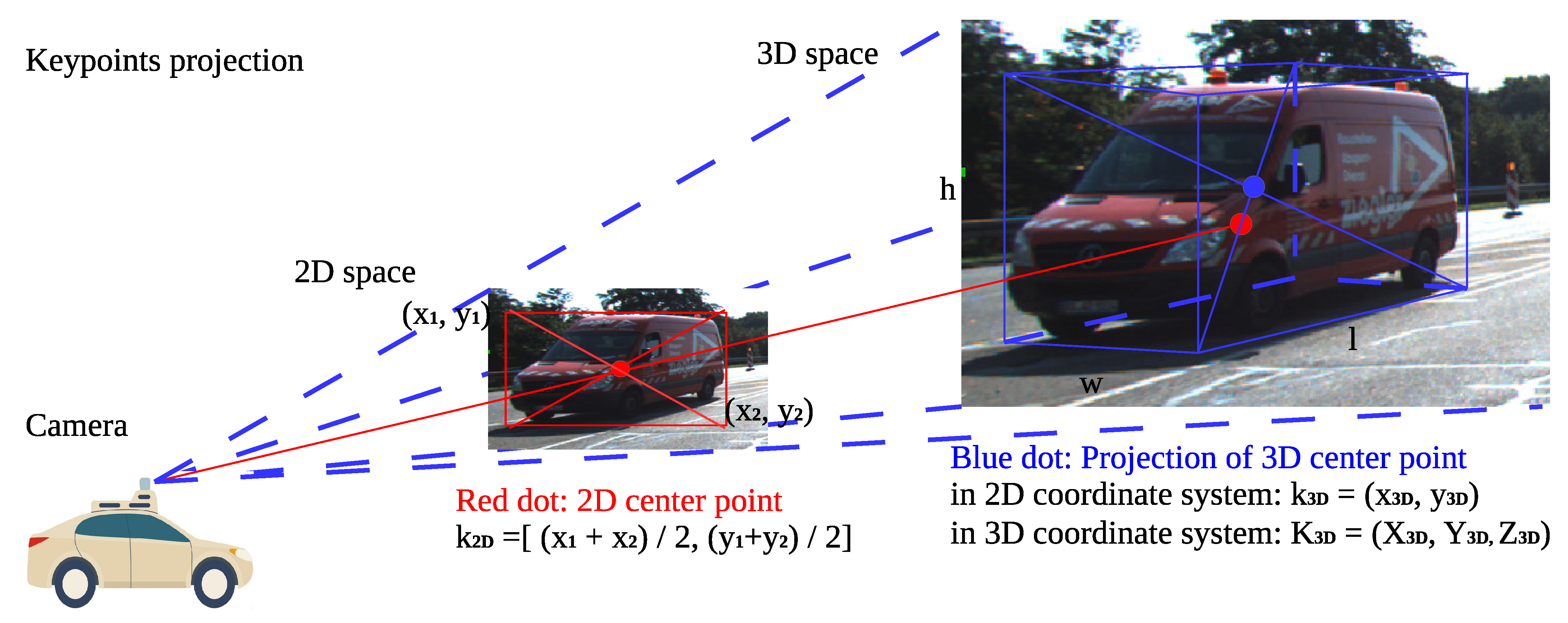
According to the principle of optical imagery, the real 3D world is mapped and condensed into 2D image planes. However, 3D geometric information is severely lost at the depth dimension during imagery projection. Considering the ground truth labels provided by training data, object n in the image can be marked by ( x 1 n , y 1 n , x 2 n , y 2 n ) , and c n for objects regression and classification, respectively. As we can see in Figure 2, the former anchor-based methods generally used 2D anchor boxes ( x 2 n x 1 n , y 2 n y 1 n ) , or 3D anchor boxes ( w , h , l ) for preset proposals. Our proposed anchor-free method leveraged keypoints to model objects for subsequent detection, without adding redundant anchor boxes with additional properties. Therefore, keypoints as the foundation of the entire system are of great significance, considering subsequent depth estimation and objects’ localization. Unlike the two keypoints proposed in CornerNet [43], we select only one keypoint in our pipeline to simplify the keypoints classification work to a great extent. The 2D center point k 2 D n = ( x 1 n + x 2 n 2 , y 1 n + y 2 n 2 ) and the projected 3D geometric center point k 3 D n = ( x 3 D n , y 3 D n ) are hardly at the same position, which makes great difference for objects detection. For 3D tasks, we instinctively select the 3D geometric center point K 3 D n = ( X 3 D n , Y 3 D n , Z 3 D n ) in the world coordinate system to anchor object n. The 3D keypoints K 3 D n in the world coordinate system are projected to 2D image plane as k 3 D n , via the transformation matrices of camera intrinsics K 3 × 4 and extrinsics R 3 × 3 , T 3 × 1 . K 3 × 4 denotes the inherent parameters inside cameras, while R 3 × 3 and T 3 × 1 represent the rotation and translation transformations, respectively. The transformation from 3D to 2D keypoint is shown in Equation (1). z c represents the depth value from the camera to objects.
z c x 3 D y 3 D 1 = K 3 × 4 R 3 × 3 T 3 × 1 0 1 X 3 D Y 3 D Z 3 D 1

3.2.2. Heatmap

Images shot by a monocular camera are first resized into the unified width W and height H for convenience of network processing. The heatmaps are generated by the backbone network, and take the responsibility for keypoints localization. Keypoint3D is aimed as a multi-category 3D object detector. Therefore, heatmaps should be designed to contain three additional channels for detecting pedestrians, cyclists, and cars, respectively. In heatmaps, keypoints are responsible for modeling objects in one-to-one correspondence. Therefore, for each object, the pixel value of keypoint can be marked as 1 and background pixels are all marked as 0 in a heatmap. Hence, we splat all ground-truth keypoints onto a heatmap H ^ [ 0 , 1 ] W 4 × H 4 × 3 , where W 4 and H 4 are the output heatmaps size, reduced by the output stride 4. We utilized DLA-34 as the basic backbone network, which could produce a high resolution of heatmaps for better performance on small objects detection.

3.2.3. Self-Adapting Ellipse Gaussian Filter

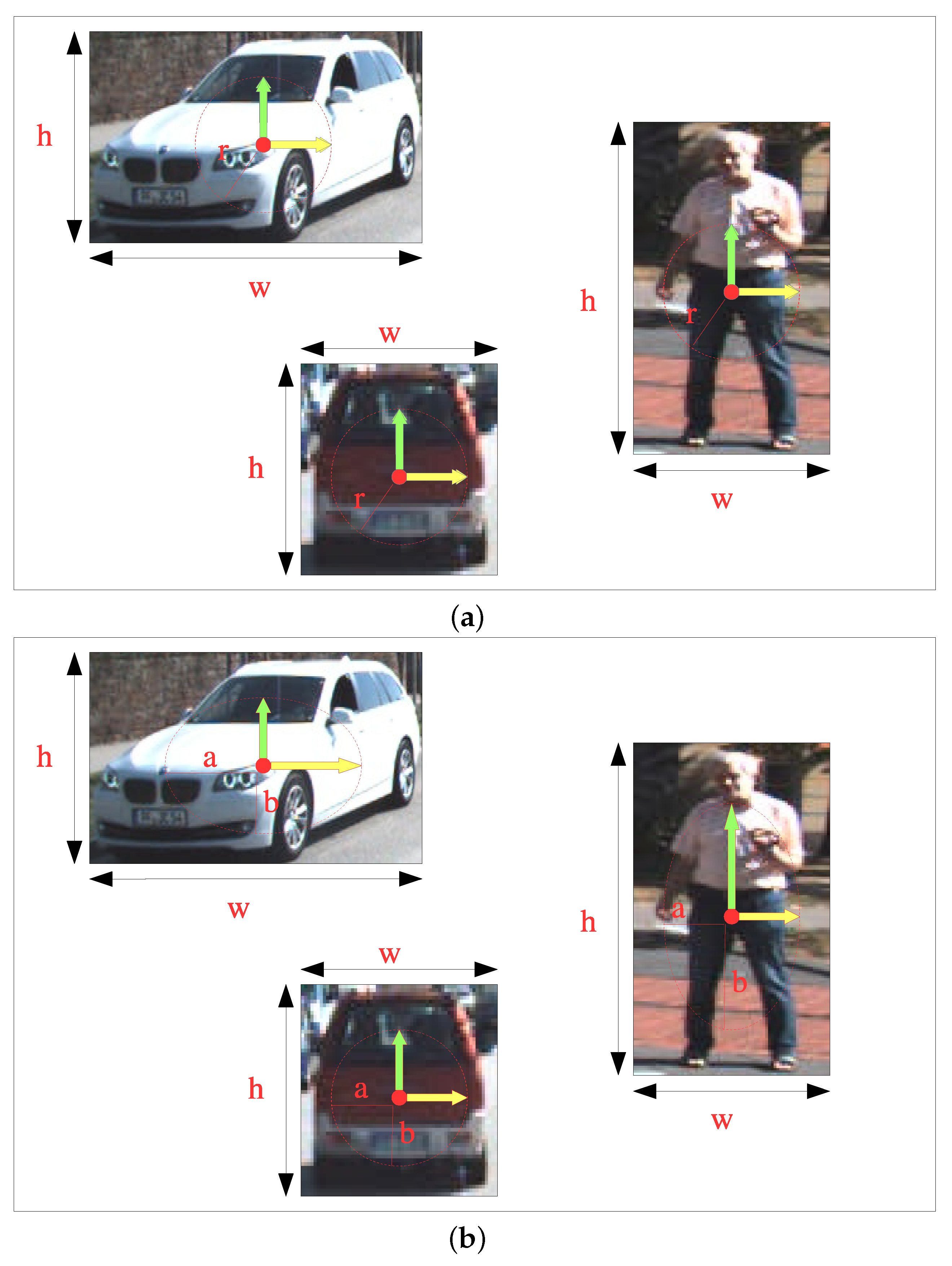
However, the contrast between 0 and 1 set in heatmaps is so sharp, which increases the difficulty of keypoints localization. Therefore, we used the Gaussian filter to apply a Gaussian blur processing, where the values of pixels around keypoints are gradually varied from 1 to 0, while the traditional methods [43,45] make Gaussian blur processing within a circle area around keypoints. Nevertheless, almost all the ground-truth boxes on 2D images are rectangles, instead of squares. Thus, it is better to use the self-adapting ellipse shapes to locate keypoints of objects, as shown in Figure 3. To be more specific, (a) presents the traditional Gaussian filter to locate keypoints of objects, which definitely performs worse on rectangular objects due to the restriction of algorithms. We improved the traditional Gaussian algorithm to be more self-adapted for rectangular shape objects in (b), which generally occupy the majority among all the objects. Different from the radius of circles r, the proposed self-adapting ellipse Gaussian filter (saEGF) has two Gaussian kernel radii a and b, which are equally scaled from the corresponding ground-truth boxes. Then, we obtain the object size-adaptive standard deviation σ a and σ b . The self-adapting ellipse Gaussian kernel (saEGF) is defined in Equation (2), where p ˜ x and p ˜ y represent the ground-truth keypoints; Y x y c denotes the saEGF kernel on the heatmap of channel c.
Y x y c = e x p ( ( x p ˜ x ) 2 2 σ a 2 ( y p ˜ y ) 2 2 σ b 2 )

3.3. Backbone

3.3.1. Semi-Aggregation Network Structure

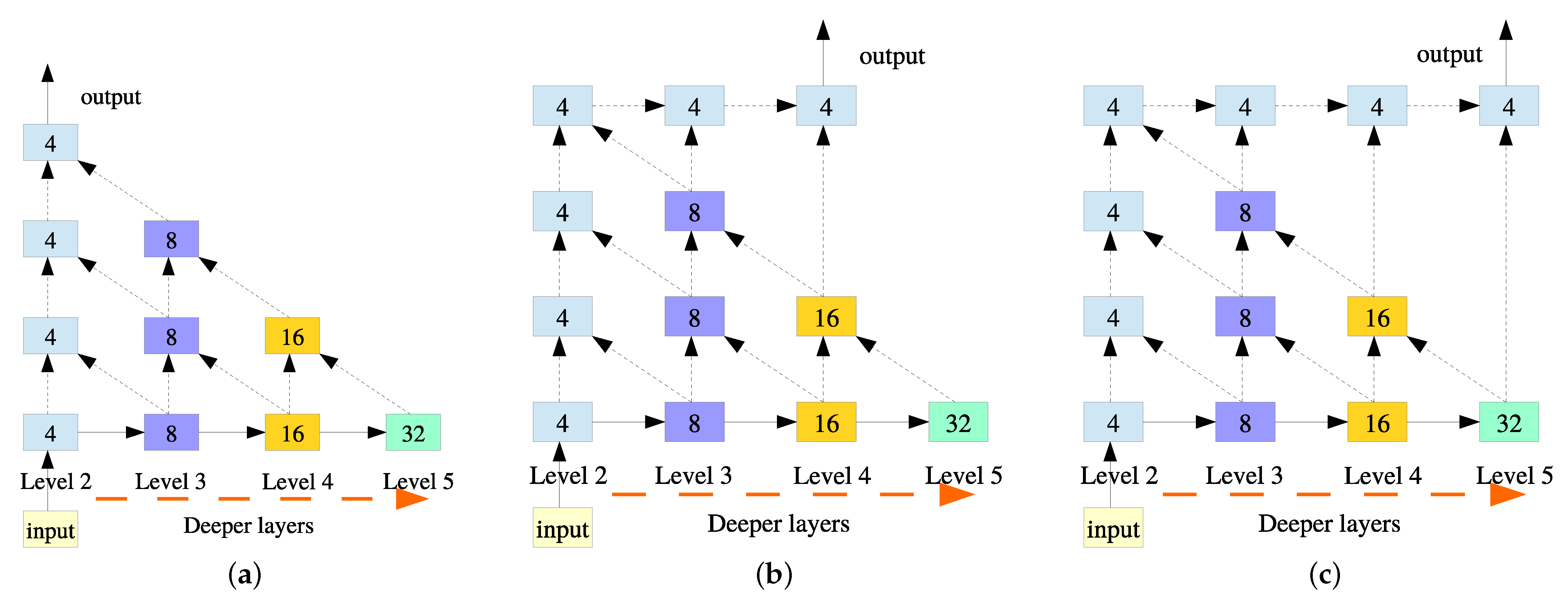
Deep layer aggregation (DLA) [51] as an image classification network makes great contribution to keypoints localization in our work. We applied the DLA-34 network as a backbone to take full advantage of the extracted features across different layers, benefited from the hierarchical information aggregation structure. The output size of the feature map is downsampled 4 times compared to original images. The high-resolution outputs also benefit to regression accuracy at the detection head stage. In this paper, we adjusted the multi-layer iterative aggregation strategy and improved the DLA-34 backbone to achieve better detection accuracy with a more simplified structure. As we can see in Figure 4, the left side network is the original DLA-34 backbone structure. The right side is the DLA-34 network applied in CenterNet [45], which completely aggregates all four hierarchical layers for a deep fusion of all features. In this paper, we empirically proposed a semi-aggregation DLA-34 backbone in the middle of Figure 4, named SADLA-34. SADLA-34 cuts the direct connection with the deepest layer and the final outputting and fuses only 3 layers of feature maps. The hierarchical structure extracted four different scales of features, where shallow layers tend to preserve more semantic features and deep layers contain more object position features. For 3D object detection, the deepest layer position-rich features are beneficial to precise keypoints localization. Nevertheless, the final output from the backbone diminished the effects of semantic features, which leads to a worse detection performance for 3D detection.
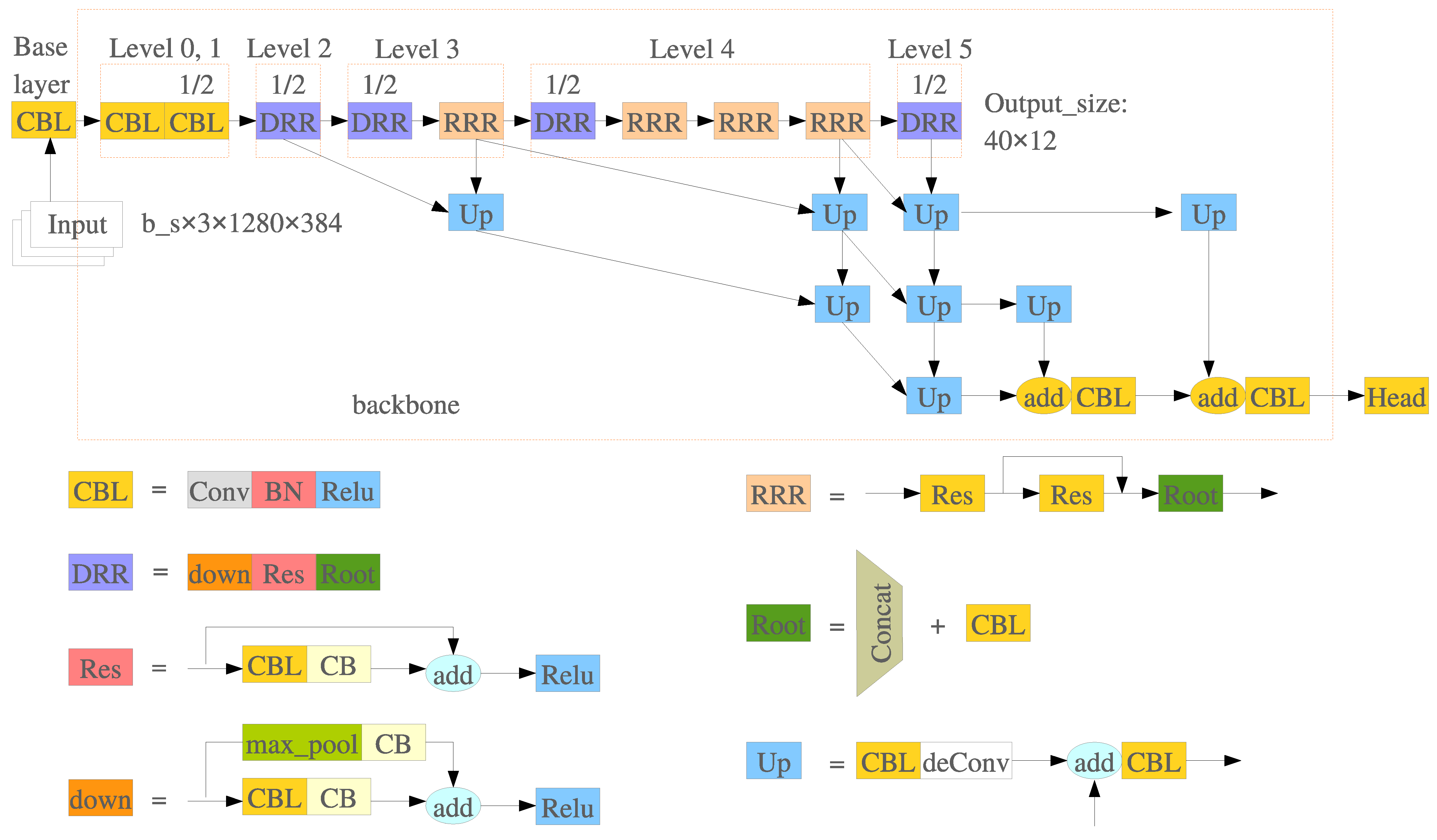
The modified SADLA-34 backbone structure is illustrated in Figure 5. After a base layer, our proposed SADLA-34 can be divided into six levels from L 0 to L 5 . L 0 and L 1 layers share the same structure body, but the convolution stride is set as 2 in the L 1 layer. From L 2 to L 5 layers, the convolution structure body starts to contain the downsampling layers and the ResNet structure [52] to enlarge receptive fields and fuse multi-scale feature maps. In L 3 and L 4 layers, we also deepened the backbone network to extract more locating information for keypoints. The hierarchical aggregation structure used iterative deep aggregation to symmetrically increase the feature maps resolution and fused different hierarchical features at different layers.

3.3.2. Deformable Convolution

Traditional neural networks used conventional convolution kernels to extract features at areas of the same size. However, traditional convolution operations cannot counter space affine transformations, such as translation, rotation, scaling, crop, and projection, leading to an unstable detection performance. To extract effective features and achieve more robust results from complex autonomous driving scenes, deformable convolution network (DCN) [53] is adopted to our backbone network for a great improvement of receptive field. As is shown in Figure 6, the 3 × 3 DCN module adds 9 learnable offsets of the deformable convolution kernel, which makes it possible for searching more valuable features on a larger convolution scale. These additional learnable offsets can be updated through gradient descent algorithm such as the parameters w and b in traditional CNN operators. In addition, the new generated offsets variables will be arranged in feature maps of 2 N channels, waiting for the next DCN operation. DCN possesses a lightweight structure that does not significantly increase the number of parameters and FLOPs in the model. We used the 3 × 3 DCN to replace traditional convolution operations at each upsampling layer.
Figure 5. Semi-aggregation DLA-34 (SADLA-34) backbone structure. SADLA-34 can be divided into L 0 L 5 levels and the iterative deep aggregation structure. We summarized each repetitive module and represented as ‘CBL’, ‘DRR’, and ‘RRR’, which can be further split into basic network units.
Remotesensing 15 01210 g005

3.4. Detection Head

Keypoint3D is aimed for a multi-category 3D detection for autonomous driving application. Additionally, we also embedded a 2D detection task into our pipeline for acquiring more comprehensive information. We demonstrated the detection head for 3D and 2D bounding boxes regression.

3.4.1. 3D Detection

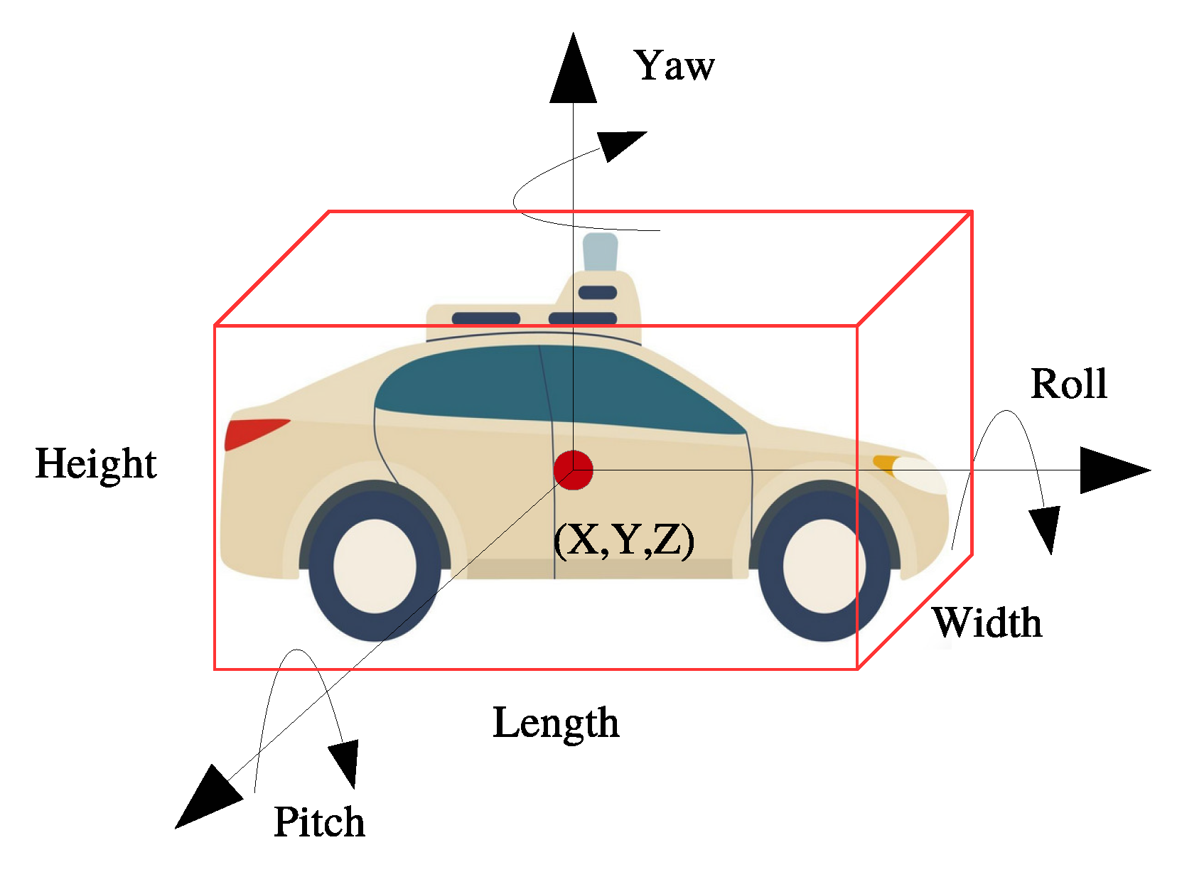
The complete 3D object detection needs to acquire 3D localization, scale, and pose information in the world coordination system. As Figure 7 shows, a 3D bounding box contains 9 Degrees of Freedom (DoF) geometric information: 3 DoF for central point coordinates, 3 DoF for cube scales, and 3 DoF for rotation angles around three axis. For unmanned aircraft tasks, 3D detection needs to detect all abovementioned DoF. Nevertheless, an autonomous vehicle does not have much parameter variations on pitch and roll rotation angles, which could not cause significantly effects in real transportation scenes. Hence, we only need to care about seven DoF for a normal autonomous vehicle and the 7-tuple vector should be represented as ( x 3 D , y 3 D , z 3 D , w , h , l , y a w ) in 3D space. Therefore, we decide to encode the 3D bounding box with a 8-tuple vector ( δ x 2 D , δ y 2 D , d a b s , w , h , l , y i m , y r e ) in 2D image coordinate system. Therefore, δ x and δ y denote the offsets for fine-turning of the localization of keypoints; d a b s and ( w , h , l ) represent the absolute depth at keypoint pixel and 3D scales for bounding boxes, respectively. We regress yaw angles of 3D bounding boxes in a Euclidean space and two parameters ( y i m , y r e ) are applied to calculate yaw angles of objects with trigonometric functions.
Keypoints classification as the core detection element for the whole 3D bounding box detection, the detection accuracy for keypoints determines the final detection performance. For further refinement of keypoints detection, we additionally added two more channels for heatmaps to regress the local offsets to correct the former detected keypoints ( x ^ 3 D , y ^ 3 D ) . Our network outputs 2 feature maps for two offsets ( δ x 3 D , δ y 3 D ) of projected keypoints in k o f f s e t H ^ W 4 × H 4 × 2 . The equation for keypoints detection is shown below:
x 3 D y 3 D = x ^ 3 D y ^ 3 D + δ x 3 D δ y 3 D
For 3D localization of keypoints, z 3 D needs to be achieved through depth prediction method. Our network outputs a feature map for depth in d H ^ W 4 × H 4 × 1 . Due to the monocular camera, absolute depth value d a b s cannot be received directly. Because the absolute depth d a b s is a variable from 0 to infinity, which is a extremely hard regression task. Therefore, inspired by the geometric transformation of depth in Eigen et al. [54], absolute depth d a b s could be transformed to normalized depth d n o r m in the range of [ 0 , 1 ] by Equation (4).
d n o r m = 1 / s i g m o i d ( d a b s ) 1
With the depth value achieved, we could recover the 3D keypoints in the world coordinate system from the projected keypoints in 2D image plane. The recovered keypoint coordinates in 3D space could be used for the loss function calculation. We applied the inverse transformation matrix to obtain the 3D coordinates in Equation (5), with the camera intrinsics K 3 × 4 and extrinsics R 3 × 3 , T 3 × 1 .
X 3 D Y 3 D Z 3 D 1 = R 3 × 3 T 3 × 1 0 1 1 K 4 × 3 1 z c x 3 D y 3 D 1
As for the anchor-free network structure, we have no presetting anchor boxes to make bounding boxes refinement. Hence, the 3D detection head directly regressed the 3D bounding box metrics, such as width w, length l, and height h. The network outputs three channels of feature maps for 3D bounding box metrics in D H ^ W 4 × H 4 × 3 .
The yaw angle regression method used in CenterNet [45] is too complicated and proved not much effective for detection accuracy. Specifically, the yaw angle is encoded with eight scalars, where four scalars are for two angles classification and the remaining four scalars are responsible for regressing the classified two angles. Finally, the yaw angle can be calculated with the abovementioned two angles with geometric transformation. Therefore, Keypoint3D introduces a much more simplified yaw regression method and still reached a competitive accuracy. As shown in Figure 8, the yaw angle is placed in a Euclidean space and represented with two variables. The two variables are placed in a complex number field, where the two axis of I m and R e denote the imaginary and real components, respectively. Moreover, we can regress the yaw angle in a completely closed mathematical space, which avoids the unnecessary occurrence of singularities. Because, two parameters are both in the range of [ 1 , 1 ] and each yaw angle matches with a unique set of two parameters on I m and R e axis. Our proposed yaw regression strategy could also save six variables compared with method in CenterNet [45]. Our network outputs feature maps for the yaw angle in Y H ^ W 4 × H 4 × 2 .
Finally, we can construct the eight corners of the 3D bounding box B in the camera frame using the yaw rotation matrix Y θ 3 × 3 , objects scales S 3 D 3 × 8 , and keypoints location K 3 D = ( X 3 D , Y 3 D , Z 3 D ) T . The regressed 3D bounding boxes will first be rotated with a rotation matrix and then translated by 3D keypoints K 3 D . Hence, the eight corners can be calculated and represented in Equations (6) and (7).
B 3 D = Y θ S 3 D + K 3 D
B 3 D = c o s ( y a w ) s i n ( y a w ) 0 s i n ( y a w ) c o s ( y a w ) 0 0 0 1 l 2 l 2 l 2 l 2 l 2 l 2 l 2 l 2 w 2 w 2 w 2 w 2 w 2 w 2 w 2 w 2 h 2 h 2 h 2 h 2 h 2 h 2 h 2 h 2 + X 3 D Y 3 D Z 3 D

3.4.2. 2D Detection

Keypoint3D makes 3D projected keypoint detection for accuracy guarantee. The 2D object detection method also serves as an additional task for verifying the basic detection performance of our proposed model. Since there is always a gap between the 2D center and 3D projected points. On the basis of predicted 3D keypoints in 2D coordinate system ( x 3 D , y 3 D ) , we designed two offsets δ c = ( δ c 1 , δ c 2 ) for 2D center points ( x 2 D , y 2 D ) . The transformation equation is shown in Equation (8).
x 2 D y 2 D = x ^ 3 D y ^ 3 D + δ c 1 δ c 2
Hence, with the size of 2D bounding boxes S 2 D regressed, we can achieve the 2D boxes coordinates B 2 D with the location of center points k 2 D in Equation (9).
B 2 D = S 2 D + k 2 D

3.5. Loss Function

3.5.1. Classification Loss

For keypoints classification, the output heatmaps will be supervised by our produced ground-truth heatmaps through self-adapting ellipse Gaussian filter (saEGF). The positions of peak values on heatmaps represent the ground-truth for keypoints. We leveraged a penalty-reduced focal loss function [19] for logistic classification. Let h ^ i , j be the predicted score at the heatmap location ( i , j ) and h i , j be the ground-truth value of each point filtered by saEFG kernels. Define the focal loss function in Equation (10):
L o s s k = 1 N i , j ( 1 h ^ i , j ) α l o g ( h ^ i , j ) ( h i , j = 1 ) ( 1 h i , j ) β ( h ^ i , j ) α l o g ( 1 h ^ i , j ) ( h i , j < 1 )
Therefore, α and β are hyper-parameters of the focal loss, and N is the number of keypoints in the predicted image. Considering the empirical hyper-parameters setting in focal loss, we set α = 2 and β = 4 in our conducted experiments.

3.5.2. Regression Loss

We encoded the 3D bounding boxes with seven DoF ( x , y , z , h , w , l , y a w ) in 3D detection head. Even though keypoints have been classified in heatmaps, further refinement still is conducted for more accurate keypoints detection. Two additional channels are added to heatmaps for refining the offsets ( δ x 3 D , δ y 3 D ) of keypoints ( x 3 D , y 3 D ) . The offsets are trained with an L 1 loss in Equation (11).
L o f f s e t s = 1 N k = 1 n ( δ x δ ^ x + δ y δ ^ y )
For the remaining 3D bounding box properties, we also used L 1 loss function for regressing a complete 3D bounding box. The absolute depth value, the three sizes, and the yaw angle are regressed in Equations (12)–(14), respectively.
L d e p t h = 1 n k = 1 n d ^ n o r m d k
L s i z e = 1 n k = 1 n h ^ h + 1 n k = 1 n w ^ w + 1 n k = 1 n l ^ l
L y a w = 1 n k = 1 n s i n ( Θ ^ ) s i n ( Θ ) + 1 n k = 1 n c o s ( Θ ^ ) c o s ( Θ )
For the additional 2D detection task, we conducted the same regression strategy for 2D bounding boxes. L 1 loss function is also utilized for 2D center points localization and 2D sizes regression.

4. Results

The proposed 3D object detection framework is trained and evaluated on the public KITTI dataset [50]. We first introduce the implementation details of our experiments in Section 4.1. In Section 4.2, the evaluation performance on 2D, 3D, and birds’ eye view (BEV) detection of Keypoint3D are conducted and compared with state-of-the-art methods. We also conduct extensive experiments for ablation studies in Section 4.3. Finally, we represent the qualitative 3D detection results as per the KITTI test set and the real driving scenes in Section 4.4.

4.1. Implementation Details

The public KITTI 3D detection dataset provides 7481 samples for training and 7518 samples for testing, both containing image sets from four cameras and corresponding point cloud samples from a 64-beam Velodyne laser scanner [50]. In our experiments, we followed the frequently used training and validation splitting method in MV3D [37], and divided training samples into t r a i n split (3712 samples) and v a l split (3769 samples). The KITTI 3D detection dataset totally covers eight categories: car, van, truck, pedestrian, pedestrian_sitting, cyclist, tram, and misc. To improve the generalization performance of the model, we merged ‘van’ and ‘pedestrian_sitting’ into the ‘car’ and ‘pedestrian’ categories, respectively. Each category can be divided into three difficulty levels: e a s y , m o d . , and h a r d , depending on different extents of occlusion and truncation. We directly input images of the original size and uniform image size to 1280 × 384 for training and testing. Therefore, the output feature maps keeps a high resolution of 320 × 96 to improve the detection ability of small targets. The most significant thing to note is that all our works were all trained and evaluated with an Intel Xeon E5-1650 v4 CPU and a single NVIDIA GTX 1080Ti GPU. The training process costs around 21 h to converge at 140 epochs totally, and the learning rate dropped at the 90 th and 120 th epoch, respectively.

4.2. Detection Performance Evaluation

We performed numerous experiments with the KITTI dataset and comprehensively evaluated our proposed detector on the performance of 2D and 3D detection. As mentioned in Section 4.1, we trained and evaluated our model on t r a i n and v a l splits, respectively. In the multi-task evaluation, we compared Keypoint3D with other outstanding 3D detectors using a monocular camera. We set the Intersection over Union (IoU) of the predicted boxes and ground-truth to 0.5 , and the evaluation results on 2D and 3D detection are shown in Table 2. Keypoint3D achieved 39.1 % in 3D object detection on the moderate level, which is quite close to M3D-RPN [34]. We utilized the SADLA-34-DCN backbone, pruning the redundant aggregation structure, which improved the inference speed to 18.9 FPS. Although, F-PointNet (Mono) [55] could achieve extremely high 3D car detection accuracy, especially on the easy level. Our Keypoint3D also outperforms the F-PointNet (Mono) [55] with remarkable margins on the real-time inference speed. Keypoint3D achieved the best speed-accuracy trade-off with the precision and efficiency in 3D detection. In terms of 2D detection, the strategy of directly detecting projected 3D keypoints in 2D image plane resulted in lower 2D average precision, considering the comparison of CenterNet [45] and modified CenterNet (3dk). However, the overall 2D detection performance of Keypoint3D could still reach 95.8 % on the easy level of the KITTI v a l set, which demonstrated the effectiveness of our proposed network greatly.
Table 3 shows the evaluation results of 3D object detection on cars, pedestrians, and cyclists at easy, moderate, and hard levels. We compared the proposed work with baseline work CenterNet [45] and the modified CenterNet (3dk) with projected 3D keypoints. Overall, 3D detection accuracy on cars, pedestrians, and cyclists all achieved huge improvements, which can be greatly contributed to the projected 3D keypoints. CenterNet [45] aimed to present a multi-task network, ignoring the optimization to specific 3D object detection task. The utilization of projected 3D keypoints enhanced the perception of three dimensional geometry scales, proving to make excellent improvements to 3D tasks. Benefiting the proposed saEGF, our model shows an obvious advantage for detecting objects with high length–width ratios, such as pedestrians and cyclists. Keypoint3D improved the 3D detection of pedestrians and cyclists in M o d . level by 31.6 % and 40.3 % , respectively, as compared with CenterNet (3dk).
We presented the average precision of 3D object localization performance on the KITTI v a l set in Table 4. We projected the detected 3D bounding boxes onto the birds’ eye view (BEV) images to validate the 3D localization performance. Benefiting from the projected 3D keypoints strategy and the self-adapting ellipse Gaussian kernel for 3D keypoints localization, we also achieved the outstanding performance of the objects localization in BEV. The average precision of localization in BEV shows first-class results, especially in moderate and hard datasets. Nevertheless, compared with 3DOP [58] using stereo cameras and AVOD [57], our proposed work using monocular vision provides a limited performance. A visualization of BEV detection results is also shown in Figure 9, Figure 10 and Figure 11.

4.3. Ablation Studies

In this section, we conducted numerous ablation experiments to analyze the effectiveness of different components of Keypoint3D. In ablation studies, the model is trained on t r a i n split and evaluated on v a l split with car 3D detection at the moderate level. We listed all the proposed strategies in Table 5: projected 3D keypoints, SADLA-34 backbone, DCN optimizing, saEGF module, and the Eulerian yaw angle. Table 5 shows the evaluation results of our work and each strategy leads to varying degrees of positive effects on 3D detection accuracy and efficiency. The detailed analysis of the contributions of our proposals has shown that Keypoint3D achieved a comprehensive improvement for 3D detection.

4.4. Qualitative Results

4.4.1. Qualitative Results on the KITTI Validation Set

For a comprehensive comparison between our baseline work and the proposed Keypoint3D, we performed experiments on 3D and BEV object detection and presented the visualization of predicted results on the KITTI v a l set. The detection results of (a) our baseline work CenterNet [45] and (b) Keypoint3D are shown in Figure 9. For evaluating the deviation between ground truth and predicted results of two models, we visualized ground truth labels and predicted 3D bounding boxes in the same images simultaneously. Ground truth labels present cars, pedestrians, and cyclists with yellow, red, and blue boxes, respectively. The predicted results present cars, pedestrians, and cyclists with pale blue, brown, and gray boxes, respectively. The differences in 3D localization performance between the two models are more clearly represented on the corresponding BEV images. The f i r s t r o w shows the heading direction prediction mistakes of two distant cars in the baseline work. The s e c o n d r o w shows a lost target of an occluded car in the baseline work. The t h i r d r o w further demonstrates the better yaw regression ability on cyclists of our Keypoint3D. Hence, through the above comparison in detail, our proposed Keypoint3D achieved the outstanding 3D object detection performance on the KITTI v a l set.

4.4.2. Qualitative Results on the KITTI Test Set

For practical applications in autonomous driving scenes, we evaluated 3D and BEV detection performance and presented the visualization on the KITTI test set. The detection results of (a) our baseline work CenterNet [45] and (b) Keypoint3D are shown in Figure 10. The differences in 3D object detection performance between the two models are more clearly represented on the corresponding BEV images. The f i r s t r o w shows a lost target in the baseline work. The s e c o n d r o w shows a better yaw angle regression performance of vehicles. The t h i r d r o w further demonstrates the better recall and yaw regression ability of our Keypoint3D. Hence, through the above comparison in detail, our proposed work Keypoint3D achieved an overall improvement with the proposed strategies.

4.4.3. Qualitative Results on Real Driving Scenes

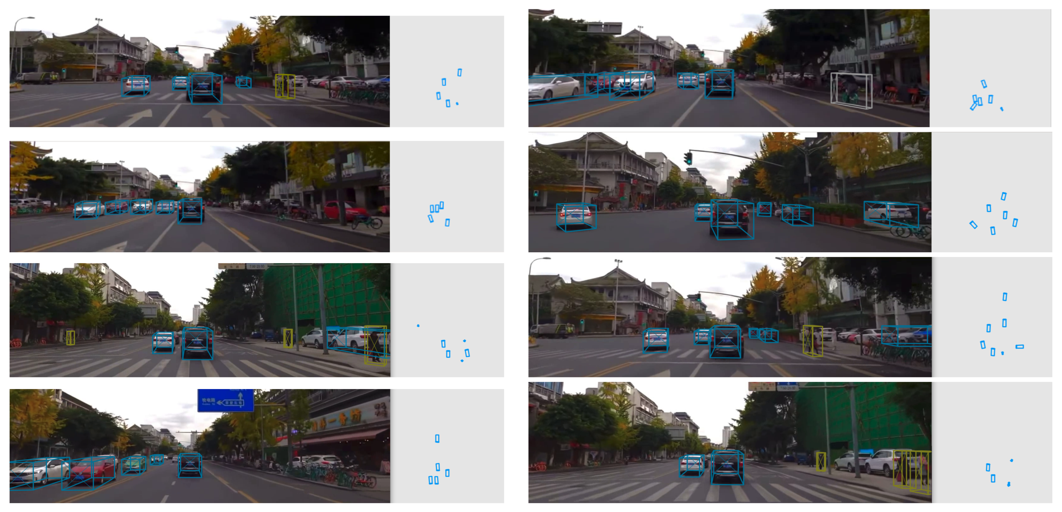
To test the generalization ability of the proposed Keypoint3D, we applied the trained model in real autonomous driving scenes. We used the real traffic scenes data from a driving vehicle equipped with a monocular camera in Chengdu, China. As shown in Figure 11, we can see 3D detection performance and corresponding results in Birds’ Eye View (BEV). The pale blue, brown, and gray boxes represent cars, pedestrians, and cyclists, respectively. Except for the missing detection in dark corners of images, 3D detection results are acceptable for a real-time testing in real application scenes.

5. Discussion

Numerous experiments conducted using the public KITTI 3D object detection dataset have proven the effectiveness of our proposed method. In the terms of 3D object detection in car category at moderate level, our proposed Keypoint3D achieves an extremely high average precision of 39.1 % in Table 2, but still shows a small margin with the state-of-the-art result of 39.6 % in M3D-RPN [34]. Benefiting from the strategies for simplifying the complexity of our model, Keypoint3D shows the best inference speed of all the state-of-the-arts as per the challenging KITTI benchmark with a NVIDIA GTX 1080Ti GPU. The outstanding performing efficiency also makes it possible for various real-time downstream applications with our proposed lightweight model. Our Keypoint3D could perform the multi-category 3D object detection for cars, pedestrians, and cyclists in Table 3. Keypoint3D makes an overall improvement on 3D object detection at all categories, compared with CenterNet [45] and the modified CenterNet (3dk). In addition, we introduce the projected 3D keypoints based network and the saEGF to improve the keypoints detection accuracy at the pixel level. As shown in Table 4, Keypoint3D represents a competitive 3D localization performance in BEV maps, which has an important influence on the final 3D detection accuracy. The 3D localization performance of our proposed method using a monocular camera almost reaches to the similar average precision of 3DOP [58] with stereo cameras. We conducted ablation studies on Keypoint3D and demonstrated the effectiveness of each single strategy on accuracy and efficiency in Table 5. With the well-trained model, we applied Keypoint3D in real driving scenes of Chengdu, China. Our Keypoint3D still presents a stable and high-performance on 3D detection in real driving scenes. In terms of the future work, we are planning to apply our Keypoint3D algorithm in IoV technique, and build a real-time and dynamic-updating traffic remote sensing system, providing the high-accuracy 3D detection information.

6. Conclusions

In this paper, we proposed an anchor-free and keypoint-based 3D object detector with monocular vision, namely Keypoint3D. We creatively leveraged projected 3D keypoints for object modeling, which improved 3D object detection accuracy greatly. Moreover, self-adapting ellipse Gaussian filter (saEGF) also made large contributions for precise keypoints positioning, considering different objects’ shapes. The proposed semi-aggregation DLA-34 (SADLA-34) network simplified the network complexity but achieved better precision performance with a faster inference speed instead. Keypoint3D regressing the yaw angle in a Euclidean space also achieved better effects on the visualization of KITTI test set. Numerous experiments on the KITTI dataset have proven that Keypoint3D achieved the best speed–accuracy trade-off with an average precision of 39.1 % at 18.9 FPS on 3D car detection at the moderate level. With a monocular camera equipped on a driving vehicle, our proposed Keypoint3D can be applied easily to complete 3D perception tasks for cars, pedestrians, and cyclists in real autonomous driving scenes and achieves extremely balanced performance.

Author Contributions

Conceptualization, Z.L. and Y.G.; methodology, Z.L.; software, Z.L.; validation, Z.L.; formal analysis, Z.L. and Y.G.; investigation, Z.L. and Q.H.; writing—original draft preparation, Z.L.; writing—review and editing, Y.D., S.S., and L.Z.; visualization, Z.L. and Y.G.; supervision, Y.D., S.S., and L.Z.; funding acquisition, Z.L. and Y.G. All authors have read and agreed to the published version of the manuscript.

Funding

This work was supported partly by the Kyushu Institute of Technology SPRING Scholarship Awardee, and partly by the University Fellowship Founding Project for Innovation Creation in Science and Technology Fellowship Program.

Data Availability Statement

The dataset generated and analyzed during the current study is available in the KITTI repository. (http://www.cvlibs.net/datasets/kitti (accessed on 20 December 2022).

Conflicts of Interest

The authors declare no conflict of interest.

References

  1. Arnold, E.; Al-Jarrah, O.Y.; Dianati, M.; Fallah, S.; Oxtoby, D.; Mouzakitis, A. A survey on 3D object detection methods for autonomous driving applications. IEEE Trans. Intell. Transp. Syst. 2019, 20, 3782–3795. [Google Scholar] [CrossRef] [Green Version]
  2. Lu, N.; Cheng, N.; Zhang, N.; Shen, X.; Mark, J.W. Connected vehicles: Solutions and challenges. IEEE Internet Things J. 2014, 1, 289–299. [Google Scholar] [CrossRef]
  3. Abdollahi, A.; Pradhan, B.; Shukla, N.; Chakraborty, S.; Alamri, A. Deep learning approaches applied to remote sensing datasets for road extraction: A state-of-the-art review. Remote Sens. 2020, 12, 1444. [Google Scholar] [CrossRef]
  4. Russell, B.J.; Soffer, R.J.; Ientilucci, E.J.; Kuester, M.A.; Conran, D.N.; Arroyo-Mora, J.P.; Ochoa, T.; Durell, C.; Holt, J. The ground to space calibration experiment (G-SCALE): Simultaneous validation of UAV, airborne, and satellite imagers for Earth observation using specular targets. Remote Sens. 2023, 15, 294. [Google Scholar] [CrossRef]
  5. Gagliardi, V.; Tosti, F.; Bianchini Ciampoli, L.; Battagliere, M.L.; D’Amato, L.; Alani, A.M.; Benedetto, A. Satellite remote sensing and non-destructive testing methods for transport infrastructure monitoring: Advances, challenges and perspectives. Remote Sens. 2023, 15, 418. [Google Scholar] [CrossRef]
  6. Guo, X.; Cao, Y.; Zhou, J.; Huang, Y.; Li, B. HDM-RRT: A fast HD-map-guided motion planning algorithm for autonomous driving in the campus environment. Remote Sens. 2023, 15, 487. [Google Scholar] [CrossRef]
  7. Mozaffari, S.; AI-Jarrah, O.Y.; Dianati, M.; Jennings, P.; Mouzakitis, A. Deep learning-based vehicle behavior prediction for autonomous driving applications: A review. IEEE Trans. Intell. Transp. Syst. 2022, 23, 33–47. [Google Scholar] [CrossRef]
  8. Jiang, Y.; Peng, P.; Wang, L.; Wang, J.; Wu, J.; Liu, Y. LiDAR-based local path planning method for reactive navigation in underground mines. Remote Sens. 2023, 15, 309. [Google Scholar] [CrossRef]
  9. Qian, R.; Lai, X.; Li, X. 3D object detection for autonomous driving: A survey. Pattern Recognit. 2022, 130, 108796. [Google Scholar] [CrossRef]
  10. Shi, S.; Wang, X.; Li, H. PointRCNN: 3D Object Proposal Generation and Detection From Point Cloud. In Proceedings of the IEEE/CVF Conference on Computer Vision and Pattern Recognition (CVPR), Long Beach, CA, USA, 16–20 June 2019; pp. 770–779. [Google Scholar] [CrossRef]
  11. Yang, Z.; Sun, Y.; Liu, S.; Shen, X.; Jia, J. STD: Sparse-to-dense 3D Object Detector for Point Cloud. In Proceedings of the IEEE/CVF International Conference on Computer Vision (ICCV), Seoul, Republic of Korea, 27 October–2 November 2019; pp. 1951–1960. [Google Scholar] [CrossRef]
  12. Wang, Z.; Jia, K. Frustum ConvNet: Sliding Frustums to Aggregate Local Point-wise Features for Amodal 3D Object Detection. In Proceedings of the IEEE/RSJ International Conference on Intelligent Robots and Systems (IROS), Macau, China, 4–8 November 2019; pp. 1742–1749. [Google Scholar] [CrossRef]
  13. Gählert, N.; Wan, J.J.; Jourdan, N.; Finkbeiner, J.; Franke, U.; Denzler, J. Single-shot 3D Detection of Vehicles from Monocular RGB Images via Geometry Constrained Keypoints in Real-time. In Proceedings of the IEEE Intelligent Vehicles Symposium (IV), Las Vegas, GA, USA, 19 October–13 November 2020; pp. 437–444. [Google Scholar] [CrossRef]
  14. Qian, R.; Garg, D.; Wang, Y.; You, Y.; Belongie, S.; Hariharan, B.; Campbell, M.; Weinberger, K.Q.; Chao, W. End-to-end Pseudo-LiDAR for Image-based 3D Object Detection. In Proceedings of the IEEE/CVF Conference on Computer Vision and Pattern Recognition (CVPR), Seattle, WA, USA, 14–19 June 2020; pp. 5881–5890. [Google Scholar] [CrossRef]
  15. Sun, J.; Chen, L.; Xie, Y.; Zhang, S.; Jiang, Q.; Zhou, X.; Bao, H. Disp R-CNN: Stereo 3D Object Detection via Shape Prior Guided Instance Disparity Estimation. In Proceedings of the IEEE/CVF Conference on Computer Vision and Pattern Recognition (CVPR), Seattle, WA, USA, 14–19 June 2020; pp. 10545–10554. [Google Scholar] [CrossRef]
  16. Chen, Y.; Shu, L.; Shen, X.; Jia, J. DSGN: Deep Stereo Geometry Network for 3D Object Detection. In Proceedings of the IEEE/CVF Conference on Computer Vision and Pattern Recognition (CVPR), Seattle, WA, USA, 14–19 June 2020; pp. 12533–12542. [Google Scholar] [CrossRef]
  17. Briñón-Arranz, L.; Rakotovao, T.; Creuzet, T.; Karaoguz, C.; EI-Hamzaoui, O. A methodology for analyzing the impact of crosstalk on LiDAR measurements. IEEE Sens. J. 2021, 1–4. [Google Scholar] [CrossRef]
  18. Zablocki, É.; Ben-Younes, H.; Pérez, P.; Cord, M. Explainability of deep vision-based autonomous driving systems: Review and challenges. Int. J. Comput. Vis. 2022, 130, 2425–2452. [Google Scholar] [CrossRef]
  19. Lin, T.Y.; Goyal, P.; Girshick, R.; He, K.; Dollár, P. Focal Loss for Dense Object Detection. In Proceedings of the IEEE International Conference on Computer Vision (ICCV), Venice, Italy, 22–29 October 2017; pp. 2999–3007. [Google Scholar] [CrossRef] [Green Version]
  20. Liu, W.; Anguelov, D.; Erhan, D.; Szegedy, C.; Reed, S.; Fu, C.Y.; Berg, A.C. SSD: Single Shot MultiBox Detector. In Proceedings of the European Conference on Computer Vision (ECCV), Amsterdam, The Netherlands, 10–16 October 2016; pp. 21–37. [Google Scholar] [CrossRef] [Green Version]
  21. Redmon, J.; Farhadi, A. YOLO9000: Better, Faster, Stronger. In Proceedings of the IEEE Conference on Computer Vision and Pattern Recognition (CVPR), Honolulu, HI, USA, 21–26 July 2017; pp. 7263–7271. [Google Scholar] [CrossRef]
  22. Redmon, J.; Farhadi, A. Yolov3: An incremental improvement. arXiv 2018, arXiv:1804.02767. [Google Scholar] [CrossRef]
  23. Bochkovskiy, A.; Wang, C.Y.; Liao, H.Y.M. YOLOv4: Optimal speed and accuracy of object detection. arXiv 2020, arXiv:2004.10934. [Google Scholar] [CrossRef]
  24. Wang, C.Y.; Bochkovskiy, A.; Liao, H.Y.M. YOLOv7: Trainable bag-of-freebies sets new state-of-the-art for real-time object detectors. arXiv 2022, arXiv:2207.02696. [Google Scholar] [CrossRef]
  25. Girshick, R.; Donahue, J.; Darrell, T.; Malik, J. Rich Feature Hierarchies for Accurate Object Detection and Semantic Segmentation. In Proceedings of the IEEE/CVF Conference on Computer Vision and Pattern Recognition (CVPR), Columbus, OH, USA, 23–28 June 2014; pp. 580–587. [Google Scholar] [CrossRef]
  26. Girshick, R. Fast R-CNN. In Proceedings of the IEEE International Conference on Computer Vision (ICCV), Santiago, Chile, 7–13 December 2015; pp. 1440–1448. [Google Scholar] [CrossRef]
  27. Ren, S.; He, K.; Girshick, R.; Sun, J. Faster R-CNN: Towards real-time object detection with region proposal networks. Adv. Neural Inf. Process. Syst. 2015, 91–99. [Google Scholar] [CrossRef] [PubMed] [Green Version]
  28. Elaksher, A.; Ali, T.; Alharthy, A. A quantitative assessment of LiDAR data accuracy. Remote Sens. 2023, 15, 442. [Google Scholar] [CrossRef]
  29. Simony, M.; Milzy, S.; Amendey, K.; Gross, H.M. Complex-YOLO: Real-time 3D Object Detection on Point Clouds. In Proceedings of the IEEE/CVF Conference on Computer Vision and Pattern Recognition (CVPR), Salt Lake City, UT, USA, 18–22 June 2018. [Google Scholar] [CrossRef]
  30. Qi, C.R.; Su, H.; Mo, K.; Guibas, L.J. PointNet: Deep Learning on Point Sets for 3D Classification and Segmentation. In Proceedings of the IEEE/CVF Conference on Computer Vision and Pattern Recognition (CVPR), Honolulu, HI, USA, 21–26 July 2017; pp. 652–660. [Google Scholar] [CrossRef]
  31. Qi, C.R.; Yi, L.; Su, H.; Guibas, L.J. PointNet++: Deep hierarchical feature learning on point sets in a metric space. arXiv 2017, arXiv:1706.02413. [Google Scholar] [CrossRef]
  32. Qin, Z.; Wang, J.; Lu, Y. MonoGRNet: A general framework for monocular 3D object detection. IEEE Trans. Pattern Anal. Mach. Intell. 2022, 44, 5170–5184. [Google Scholar] [CrossRef]
  33. Yan, C.; Salman, E. Mono3D: Open source cell library for monolithic 3-D integrated circuits. IEEE Trans. Circuits Syst. 2018, 65, 1075–1085. [Google Scholar] [CrossRef]
  34. Brazil, G.; Liu, X. M3D-RPN: Monocular 3D Region Proposal Network for Object Detection. In Proceedings of the IEEE/CVF International Conference on Computer Vision (ICCV), Seoul, Republic of Korea, 27 October–2 November 2019; pp. 9286–9295. [Google Scholar] [CrossRef] [Green Version]
  35. Liu, Y.; Wang, L.; Liu, M. YOLOStereo3D: A Step Back to 2D for Efficient Stereo 3D Detection. In Proceedings of the IEEE International Conference on Robotics and Automation (ICRA), Xi’an, China, 30 May–5 June 2021; pp. 13018–13024. [Google Scholar] [CrossRef]
  36. Vora, S.; Lang, A.H.; Helou, B.; Beijbom, O. PointPainting: Sequential Fusion for 3D Object Detection. In Proceedings of the IEEE/CVF Conference on Computer Vision and Pattern Recognition (CVPR), Seattle, WA, USA, 14–19 June 2020; pp. 4603–4611. [Google Scholar] [CrossRef]
  37. Chen, X.; Ma, H.; Wan, J.; Li, B.; Xia, T. Multi-view 3D Object Detection Network for Autonomous Driving. In Proceedings of the IEEE Conference on Computer Vision and Pattern Recognition (CVPR), Honolulu, HI, USA, 21–26 July 2017; pp. 1907–1915. [Google Scholar] [CrossRef]
  38. Pang, S.; Morris, D.; Radha, H. CLOCs: Camera-LiDAR Object Candidates Fusion for 3D Object Detection. In Proceedings of the IEEE/RSJ International Conference on Intelligent Robots and Systems (IROS), Las Vegas, NV, USA, 25–29 October 2020; pp. 10386–10393. [Google Scholar] [CrossRef]
  39. Hartigan, J.A.; Wong, M.A. Algorithm AS 136: A K-means clustering algorithm. J. R. Stat. Soc. C Appl. Stat. 1979, 28, 100–108. [Google Scholar] [CrossRef]
  40. Mousavian, A.; Anguelov, D.; Flynn, J. 3D bounding box estimation using deep learning and geometry. arXiv 2017, arXiv:1612.00496. [Google Scholar] [CrossRef]
  41. Chabot, F.; Chaouch, M.; Rabarisoa, J.; Teuliere, C.; Chateau, T. Deep Manta: A Coarse-to-fine Many Task Network for Joint 2D and 3D Vehicle Analysis from Monocular Image. In Proceedings of the IEEE Conference on Computer Vision and Pattern Recognition (CVPR), Honolulu, HI, USA, 21–26 July 2017; pp. 2040–2049. [Google Scholar] [CrossRef]
  42. Lang, A.H.; Vora, S.; Caesar, H. Pointpillars: Fast Encoders for Object Detection from Point Clouds. In Proceedings of the IEEE/CVF Conference on Computer Vision and Pattern Recognition (CVPR), Long Beach, CA, USA, 16–20 June 2019; pp. 12697–12705. [Google Scholar] [CrossRef]
  43. Law, H.; Deng, J. Cornernet: Detecting Objects as Paired Keypoints. In Proceedings of the European Conference on Computer Vision (ECCV), Munich, Germany, 8–14 September 2018; pp. 734–750. [Google Scholar] [CrossRef]
  44. Lin, T.Y.; Maire, M.; Belongie, S. Microsoft COCO: Common Objects in Context. In Proceedings of the European Conference on Computer Vision (ECCV), Zurich, Switzerland, 5–12 September 2014; pp. 740–755. [Google Scholar] [CrossRef]
  45. Zhou, X.; Wang, D.; Krähenbühl, P. Objects as points. arXiv 2019, arXiv:1904.07850. [Google Scholar] [CrossRef]
  46. Li, P.; Zhao, H.; Liu, P.; Cao, F. RTM3D: Real-time Monocular 3D Detection from Object Keypoints for Autonomous Driving. In Proceedings of the European Conference on Computer Vision (ECCV), Online, 23–28 August 2020; pp. 644–660. [Google Scholar] [CrossRef]
  47. Caesar, H.; Bankiti, V.; Lang, A.H.; Vora, S.; Liong, V.E.; Xu, Q.; Krishnan, A.; Pan, Y.; Baldan, G.; Beijbom, O. nuScenes: A Multimodal Dataset for Autonomous Driving. In Proceedings of the IEEE/CVF Conference on Computer Vision and Pattern Recognition (CVPR), Seattle, WA, USA, 14–19 June 2020; pp. 11618–11628. [Google Scholar] [CrossRef]
  48. Patil, A.; Malla, S.; Gang, H.; Chen, Y. The H3D Dataset for Full-Surround 3D Multi-Object Detection and Tracking in Crowded Urban Scenes. In Proceedings of the International Conference on Robotics and Automation (ICRA), Montreal, QC, Canada, 20–24 May 2019; pp. 9552–9557. [Google Scholar] [CrossRef]
  49. Sun, P.; Kretzschmar, H.; Dotiwalla, X.; Chouard, A.; Patnaik, V.; Tsui, P.; Guo, J.; Zhou, Y.; Chai, Y.; Caine, B.; et al. Scalability in Perception for Autonomous Driving: Waymo Open Dataset. In Proceedings of the IEEE/CVF Conference on Computer Vision and Pattern Recognition (CVPR), Seattle, WA, USA, 14–19 June 2020; pp. 2446–2454. [Google Scholar] [CrossRef]
  50. Geiger, A.; Lenz, P.; Urtasun, R. Are We Ready for Autonomous Driving? The KITTI Vision Benchmark Suite. In Proceedings of the IEEE/CVF Conference on Computer Vision and Pattern Recognition (CVPR), Providence, RI, USA, 16–21 June 2012; pp. 3354–3361. [Google Scholar] [CrossRef]
  51. Yu, F.; Wang, D.; Shelhamer, E.; Darrell, T. Deep Layer Aggregation. In Proceedings of the IEEE/CVF Conference on Computer Vision and Pattern Recognition (CVPR), Salt Lake City, UT, USA, 18–22 June 2018; pp. 2403–2412. [Google Scholar] [CrossRef]
  52. He, K.; Zhang, X.; Ren, S. Deep Residual Learning for Image Recognition. In Proceedings of the IEEE Conference on Computer Vision and Pattern Recognition (CVPR), Las Vegas, NV, USA, 26 June–1 July 2016; pp. 770–778. [Google Scholar] [CrossRef]
  53. Wang, R.; Shivanna, R.; Cheng, D.Z.; Jain, S.; Lin, D.; Hong, L.; Chi, E.H. DCN V2: Improved Deep and Cross Network and Practical Lessons for Web-scale Learning to Rank Systems. In Proceedings of the Web Conference, Ljubljana, Slovenia, 12–23 April 2021; pp. 1785–1797. [Google Scholar] [CrossRef]
  54. Eigen, D.; Puhrsch, C.; Fergus, R. Depth map prediction from a single image using a multi-scale deep network. arXiv 2014, arXiv:1406.2283. [Google Scholar] [CrossRef]
  55. Qi, C.R.; Liu, W.; Wu, C.; Su, H.; Guibas, L.J. Frustum PointNets for 3D Object Detection From RGB-D Data. In Proceedings of the IEEE/CVF Conference on Computer Vision and Pattern Recognition (CVPR), Salt Lake City, UT, USA, 18–22 June 2018; pp. 918–927. [Google Scholar] [CrossRef]
  56. Xu, B.; Chen, Z. Multi-level Fusion based 3D Object Detection from Monocular Image. In Proceedings of the IEEE/CVF Conference on Computer Vision and Pattern Recognition (CVPR), Salt Lake City, UT, USA, 18–23 June 2018; pp. 2345–2353. [Google Scholar] [CrossRef]
  57. Ku, J.; Mozifian, M.; Lee, J.; Harakeh, A.; Waslander, S.L. Joint 3D Proposal Generation and Object Detection from View Aggregation. In Proceedings of the IEEE/RSJ International Conference on Intelligent Robots and Systems (IROS), Madrid, Spain, 1–5 October 2018; pp. 1–8. [Google Scholar] [CrossRef] [Green Version]
  58. Chen, X.; Kundu, K.; Zhu, Y.; Ma, H.; Fidler, S.; Urtasun, R. 3D object proposals using stereo imagery for accurate object class detection. IEEE Trans. Pattern Anal. Mach. Intell. 2018, 40, 1259–1272. [Google Scholar] [CrossRef] [PubMed] [Green Version]
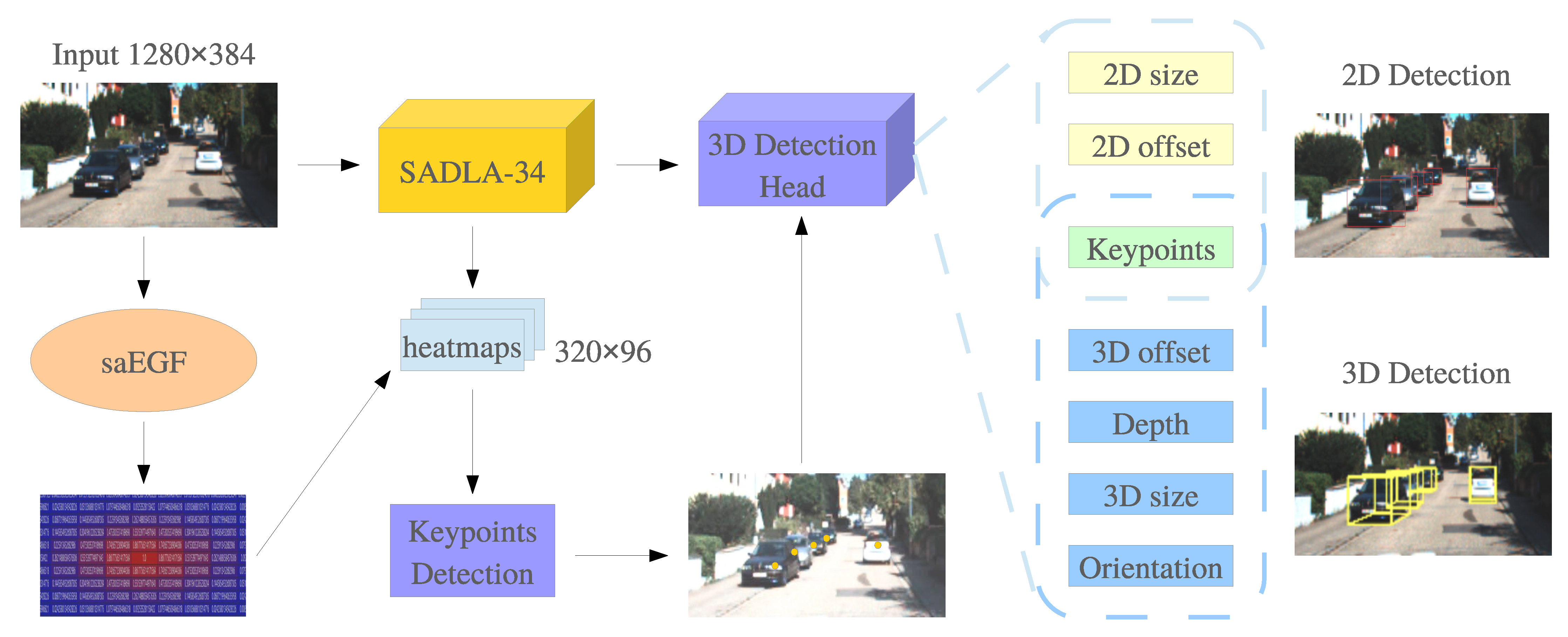
Figure 1. Architecture of the proposed 3D object detection pipeline. A single image serves as input of this framework and will firstly be processed in the SADLA-34 backbone for feature extraction. The outputting heatmaps will be used to detect keypoints of objects, according to the ground truth generated by saEGF module. The predicted keypoints will be inputted into 3D detection head to generate 3D bounding boxes with other regressed 3D properties. Additionally, 2D object detection can also be implemented in this pipeline.
Remotesensing 15 01210 g001
Figure 2. Keypoints mapping from 3D to 2D space. The red and blue dots denote the 2D center point and the projected keypoint from 3D space, respectively.
Remotesensing 15 01210 g002
Figure 3. Comparison between two Gaussian filters. (a) Traditional Gaussian filter. (b) Self-adapting ellipse Gaussian filter (saEGF).
Remotesensing 15 01210 g003
Figure 4. Comparison between three DLA-34 networks with different aggregation strategies. (a) The original DLA-34 Backbone. (b) The proposed semi-aggregation DLA-34 (SADLA-34) backbone. (c) Full-aggregation DLA-34 backbone.
Remotesensing 15 01210 g004
Figure 6. Illustration of 3 × 3 deformable convolution. Each input feature map would generate 2 N channels in offset fields. N denotes the number of arrows in offsets. Each arrow contains 2 variables for horizontal and vertical directions. w 1 w 9 are additional variables representing the offsets.
Remotesensing 15 01210 g006
Figure 7. Degree-of-freedom for 3D object detection. A full-scale 3D bounding box contains nine DoF, while 3D detection in self-driving eliminates the roll and pitch angles.
Remotesensing 15 01210 g007
Figure 8. Yaw angle regression in Euclidean space. θ represents the yaw angle of objects, which further is divided into two variables on I m and R e axis. I m and R e represent the imaginary and real components, respectively.
Remotesensing 15 01210 g008
Figure 9. Qualitative comparisons of the detection performance in 3D and BEV on the KITTI v a l set. (a) Baseline work (CenterNet). (b) The proposed method (Keypoint3D). Ground truth labels present cars, pedestrians, and cyclists with yellow, red and blue boxes, respectively. The predicted results present cars, pedestrians, and cyclists with pale blue, brown, and gray boxes, respectively. The heading direction is represented with a cross mark.
Remotesensing 15 01210 g009
Figure 10. Qualitative comparisons of the detection performance in 3D and BEV on the KITTI test set. (a) Baseline work (CenterNet). (b) The proposed method (Keypoint3D). Cars, pedestrians, and cyclists are represented by pale blue, brown, and gray boxes, respectively. The heading direction is represented with a cross mark.
Remotesensing 15 01210 g010
Figure 11. Real scenes application of the proposed Keypoint3D on the road of Chengdu, China. Cars, pedestrians, and cyclists are represented by pale blue, brown, and gray boxes, respectively. The heading direction is represented with a cross mark.
Remotesensing 15 01210 g011
Table 1. A summary of public datasets on 3D object detection in autonomous driving.
DatasetScenesClassesFrames3D BoxesYear
nuScenes [47]10002340K1.4M2019
H3D [48]160827K1.1M2019
Waymo [49]11504200K112M2020
KITTI [50]50815K200K2012
Table 2. The 2D and 3D detection performance comparison between Keypoint3D and state-of-the-art methods as per the KITTI benchmark in car category. FPS indicates the inference speed, and 3dk denotes the utilization of 3D projected keypoints in CenterNet [45]. All the methods in trained and evaluated on the KITTI t r a i n and v a l set. AP 2 D and AP 3 D indicates the 2D and 3D object detection average precision with the I o U set as 0.7 and 0.5 , respectively.
AP 2 D AP 3 D FPS
EasyMod.HardEasyMod.Hard
MonoGRNet [32]---50.537.030.816.7
Mono3D [33]92.388.779.025.218.215.5-
M3D-RPN [34]90.283.767.749.039.633.06.2
F-PointNet (Mono) [55]---66.342.338.55
MF3D [56]---47.929.526.48.3
AVOD (Mono) [57]---57.042.836.3-
CenterNet [45]97.187.979.319.518.616.615.4
CenterNet (3dk)87.185.669.839.931.430.115.4
Keypoint3D (Ours)95.887.377.848.139.132.518.9
Table 3. 3D object detection accuracy comparison of the baseline work and Keypoint3D in car, pedestrian, and cyclist categories. The average precision ( A P 3 D ) (in %) of 3D object detection is evaluated as per the KITTI v a l set ( I o U = 0.5 ).
CarPedestrianCyclist
EasyMod.HardEasyMod.HardEasyMod.Hard
CenterNet [45]19.518.616.521.016.815.819.511.810.9
CenterNet (3dk)39.931.430.131.320.417.523.116.415.9
Keypoint3D (Ours)48.139.132.537.923.919.630.423.021.1
Table 4. 3D localization performance as per the KITTI v a l set in car. The 3D location performance is evaluated by the average precision ( A P l o c ) (in %) of BEV boxes as per the KITTI v a l set ( I o U = 0.5 ).
MethodSensorsEasyMod.Hard
3DOP [58]Stereo55.041.334.6
Mono3D [33]Mono30.522.419.2
MF3D [56]Mono55.036.731.3
M3D-RPN [34]Mono55.442.535.3
AVOD [57]Mono61.245.438.3
CenterNet [45]Mono31.529.728.1
CenterNet (3dk)Mono46.837.932.7
Keypoint3D (Ours)Mono52.639.533.2
Table 5. Ablation studies of the proposed strategies. We used the verification experiments to explore the effect of the five proposed strategies at the detection accuracy and efficiency improvements.
3D KeypointSADLA-34SADLA-34-DCNsaEGFEulerian AnglemAPFPS
××××31.415.4
×××35.719.6
××36.118.0
×38.918.0
39.118.9
Disclaimer/Publisher’s Note: The statements, opinions and data contained in all publications are solely those of the individual author(s) and contributor(s) and not of MDPI and/or the editor(s). MDPI and/or the editor(s) disclaim responsibility for any injury to people or property resulting from any ideas, methods, instructions or products referred to in the content.