Abstract
Wind energy is one of Brazil’s most promising energy sources, and the rapid growth of wind plants has increased the need for accurate and efficient inspection methods. The current onsite visits, which are laborious and costly, have become unsustainable due to the sheer scale of wind plants across the country. This study proposes a novel data-centric approach integrating semantic segmentation and GIS to obtain instance-level predictions of wind plants by using free orbital satellite images. Additionally, we introduce a new annotation pattern, which includes wind turbines and their shadows, leading to a larger object size. The elaboration of data collection used the panchromatic band of the China–Brazil Earth Resources Satellite (CBERS) 4A, with a 2-m spatial resolution, comprising 21 CBERS 4A scenes and more than 5000 wind plants annotated manually. This database has 5021 patches, each with 128 × 128 spatial dimensions. The deep learning model comparison involved evaluating six architectures and three backbones, totaling 15 models. The sliding windows approach allowed us to classify large areas, considering different pass values to obtain a balance between performance and computational time. The main results from this study include: (1) the LinkNet architecture with the Efficient-Net-B7 backbone was the best model, achieving an intersection over union score of 71%; (2) the use of smaller stride values improves the recognition process of large areas but increases computational power, and (3) the conversion of raster to polygon in GIS platforms leads to highly accurate instance-level predictions. This entire pipeline can be easily applied for mapping wind plants in Brazil and be expanded to other regions worldwide. With this approach, we aim to provide a cost-effective and efficient solution for inspecting and monitoring wind plants, contributing to the sustainability of the wind energy sector in Brazil and beyond.
1. Introduction
The great challenge for the Brazilian energy sector is to expand its production capacity while maintaining a high share of renewable sources in the energy mix. One of the most critical factors is to guarantee its commitment to reduce greenhouse gas emissions (GHGs), established by the Intended Nationally Determined Contributions (INDC) [1] and in line with the Paris agreement ratified by Brazil in September 2016 [2]. Hydroelectricity has been the primary source of Brazilian energy and the main geopolitical energy strategy since the 1960s. Brazil has a notable advantage in having a hydroenergy base, a renewable, storable, and fundamental source for stability in meeting the country’s energy demand, especially because large plants are beneficial for regulating the demands at a reasonable time when the energy loads fluctuate. This development model made Brazil the nation most dependent on hydroelectric energy globally.
However, most potential hydropower sites have already been explored for energy generation, and new large-scale projects are predominantly in the Amazon region. This region imposes massive restrictions on constructing new hydropower plants in the country due to significant socioeconomic and environmental impacts, compromising fragile ecosystems and entailing high costs in the long term [3,4]. Recently, the Belo Monte project, with an installed capacity of 11.23 GW, illustrates the challenges of installing hydroelectric dams in the Amazon region. The project had a budget of US $13.1 billion and flooded an area greater than 7000 km2, presenting challenges for environmental [5,6,7,8] and socioeconomic mitigation [9,10] and demanding efforts in terms of population resettlement.
Therefore, ensuring energy security in the face of the country’s economic growth and maintaining a portfolio of renewable sources leads to a redirection of investments, efforts, and priorities for the decentralization of renewable technologies with an increase in the reliability of the supply of the electrical system and risk reduction. In this scenario, solar and wind energy acquire prominence in this reduction in hydroelectric participation and sustain a mostly renewable share in the mix as it is currently [11]. The hydroelectric source represented 83% of installed capacity at the beginning of the century, and the expectation is to reduce it to 46% by 2031, according to the Brazilian government’s Ten-Year Energy Plan (PDE-2031) [12]. Thus, the contribution of hydroelectricity in the last decade has gradually decreased for these new alternatives that have reached the gigawatt scale [13]. Moreover, relying on a single natural energy source brings security issues because these renewable energies are susceptible to climatic variations, with a possible need to activate thermoelectric plants to meet domestic demands [14,15]. Several studies point out this problem and analyze moments of the recent energy crisis in the country [13,16,17,18].
In addition, wind and solar energy allow a decentralized production closer to the consumer. Technological advances promote the constant reduction of generation costs, overcoming technical barriers and making these sources increasingly competitive due to economic gains and efficiency. Among the advantages of wind and solar energy systems are carbon-free energy sources with low environmental impact, the potential to mitigate greenhouse gas emissions, low operating and maintenance costs, high availability, the ability to strengthen the ends of the network, reduction of energy transmission losses, and increased overall efficiency of the electrical system [19]. Future projections of climate change show that in the 2030s and 2080s, there will be a decrease in rainfall for most of the Brazilian territory and an increase in solar irradiation, temperature, and wind speed compared to the previous century [20]. In this context, potential hydroelectric decreases, solar energy potential shows a slight increase, and wind energy shows a significant increase, reaching in some locations an increase in wind energy generation of more than 40% [20].
According to the Brazilian National Electricity Agency (ANEEL) data from the beginning of 2022, the number of wind power plants in operation was 809, with a granted power of 21.5 GW and supervised power of 21.4 GW, which represents 11.77% of the Brazilian energy mix. The number reaches 1190 units with a granted power of 34.9 GW from the wind farms under construction and construction not started. In Brazil, the Northeast region is the most promising and favorable for wind energy conversion due to adequate conditions, with high average wind speeds (>8.5 m/s) and a low level of turbulence throughout the year with a Weibull k factor greater than three [21]. Eight units are in the Northeast region, among the 10 states with the highest power granted in operation. The first three states are Bahia (6.5 GW), Rio Grande do Norte (5.9 GW), and Piauí (2.5 GW). Therefore, there has recently been a significant increase in wind energy exploration ventures.
Consequently, inspecting wind plant constructions is fundamental for the effectiveness and control of public policies. In Brazil, ANEEL is responsible for regulating the expansion of installed capacity and monitoring the progress of plant construction [22]. However, inspection occurs directly onsite by displacing qualified professionals at high costs. The expectation of wind energy growth tends to have many projects with low energy production, increasing the number of processes to be evaluated and urgently requiring process automation.
Thus, this research seeks to overcome three problems in the development of a system that helps the growing inspection process with significant savings and increased agility: (1) minimize the need for inspectors to travel to the construction sites by using remotely sensed data, (2) increase the accuracy of automatic mapping of wind farms employing segmentation techniques based on deep learning, and (3) wind power plants consist of small nonuniform objects in remote sensing images due to different blade positions and projected shadows, which establishes a high complexity in image-recognition results. The shades from wind power stations allow for increased detection area.
In a continental-sized country, periodic satellite images are a promising and low-cost tool for monitoring works in the electricity sector. Remote sensing studies for detecting infrastructure in the electricity sector have recently expanded, considering different energy sources. The use of remotely sensed data in solar energy mapping has shown a significant increase, such as urban photovoltaic solar panels [23,24,25,26,27], water photovoltaic [28] and photovoltaic solar plants [29,30,31], solar energy estimations [32,33,34], solar power plant site selection [35,36,37,38,39,40], and photovoltaic potential on building rooftops [41,42,43,44]. Remote sensing has also been widely used in analyzing the environmental changes in hydroelectric plants in their reservoirs and downstream of dams [3,45,46,47,48] and in maintenance of power line corridors [49,50,51,52,53]. On the other hand, wind farm detection studies are scarce, as they are small objects and require high-resolution images.
In digital image processing, a challenge is to achieve a highly accurate detection minimizing human activity, such as visual inspection and onsite visits. In this context, deep learning methods are the current state-of-the-art for image classification, especially with advances in convolutional neural networks (CNN), which allow the detection of small, medium, and high-level features [54,55]. In the electricity sector, pattern-recognition methodologies for solar panels have shown high efficiency, including studies by ANEEL [29].
Few studies used deep-learning strategies to map wind plants by using terrestrial-monitoring images [56,57,58,59]. Han et al. [59] detected wind power plants by using high-resolution Gaofen-2 fused images (with a spatial resolution of 0.8 m) and a CNN based on U-Net architecture, reaching an F1-score of 0.97. Manso–Callejo et al. [57] used aerial images and compared the U-Net and LinkNet architectures with various backbones (EfficientNet-b0, EfficientNet-b1, EfficientNet-b2, EfficientNet-b3, and SEResNeXt50), getting better results with the LinkNet-EfficientNet-b3 combination. An improvement of this research for the entire Spanish peninsular territory is presented by Manso–Callejo et al. [56], in which another multiclass recognition network classified turbines by their power capacity. In both studies developed by Manso–Callejo et al. [56,57], only the base is labeled, with no wind farm segmentation. Finally, Schulz et al. [58] used a Mask R-CNN on aerial photography images to detect decentralized renewable energies, including wind power plants. Unlike the approach of aerial or satellite images with top view, some other studies use lateral images of drones and deep learning methods for inspection analysis of imminent damage related to wind turbine blades [60,61]. In the cited studies, only one research [58] used a deep-learning segmentation method from aerial images to delineate all wind power plant features. The other studies used a single point to label each object, not configuring a segmentation task, which represents a significant gap in the use of segmentation strategies with orbital satellite images.
In addition, unlike other deep learning-based studies, this investigation focused on finding a cost-effective solution for ANEEL to conduct periodic surveys of the Brazilian territory (continental area) using free images. The solution to this problem was using China–Brazil Earth Resources Satellite (CBERS) 4A images with a resolution of 2 m, significantly worse than the aerial photographs (centimetric resolution) used in previous studies. In this context, the challenge for detection is the complexity of wind power plants combined with the reduced number of pixels representing them, belonging to the small object category (size < 32 × 32 pixels) [62,63]. Nowadays, advances and novelties in deep-learning studies either refer to data-centric or model-centric approaches. Due to the characteristics of previous studies, the most significant scientific gap is not the inaccuracy of the deep learning models but the creation of mechanisms of consistent labeling. The data-centric approach seeks to improve datasets to increase model performance, considering different strategies not limited to simply increasing the size of the datasets, such as including label reliability or incorporating detailed training data. For example, the representation of wind power plants considering only one point (a single pixel) is very difficult to maintain consistency from images with lower spatial resolution. Therefore, the solution to this small-object detection problem considered an alternative based on the data-centric approach, including the wind plant shadows to increase the mapped area and facilitate target detection. This alternative has already been used in other studies without deep semantic segmentation. Shen et al. [64] considered the shadow in monitoring wind plant constructions by using Chinese satellite GF-2 HD images and a Normalized Difference Vegetation Index (NDVI)-based method, including mask generation and interactive interpretation. Mandroux et al. [65] used dark shadows and bright hubs from wind plants for their detection in Sentinel-2 images by using adaptive thresholding.
This study aims to develop a low-cost system by using deep learning and free remote sensing images to monitor wind plants, reducing technical visits, and providing quick and accurate inspection information. The main contributions are as follows.
- A novel data-centric approach is introduced, consisting of a new strategy of annotating wind plants (including the shadows and turbines), which increases the size of the objects, facilitating the recognition. In addition, this strategy allows the use of 2-m resolution images for small-object detection. Wind plants have a low representation in nadir images, but they present an extensive shadow due to their height, which facilitates indirect detection by deep learning methods.
- A novel semantic segmentation dataset is introduced, the first considering CBERS-4A images covering the entire Brazilian territory. CBERS-4A presents the advantages of being free of charge and having a 2-m resolution for the panchromatic band. Thus, the inference procedure is much faster by only considering one band.
- A novel semantic to instance segmentation conversion using geographic information system (GIS) software. The spatial distribution of wind farms, appearing sparsely without contacts between them, makes the polygonization of the semantic features create a specific identifier per instance, in addition to favoring the removal of noisy features based on the size of the objects.
2. Materials and Methods
The present research had the following methodological steps (Figure 1): (Section 2.1) data, (Section 2.2) deep learning approach, (Section 2.3) sliding windows using the best model, and (Section 2.4) semantic to instance conversion using GIS.
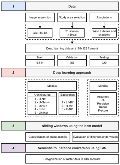
Figure 1.
Methodological flowchart. The numbering corresponds to the subtopics of the section.
2.1. Data
2.1.1. Study Area Selection and Image Acquisition
The study areas include the main concentrations of wind farms across the Brazilian territory (Figure 2). In this context, this study covered a wide variety of landscapes, from coastal areas with the presence of dunes up to inland regions with different land cover. This research used the panchromatic images of the China–Brazil Earth Resources Satellite CBERS 4A sensor (2-m resolution), the sixth CBERS family satellite developed by the space technical cooperation between Brazil and China [66]. These images combine the advantages of free distribution (significant cost reduction) and high resolution from the panchromatic wide scan camera.
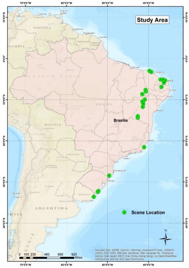
Figure 2.
Location of all 21 CBERS 4A scenes used in this study.
Other possibilities for high-resolution images, such as aerial surveys or using orbital satellites (GeoEye-1 (41 cm), WordView-2 (46 cm), WordView-3 (31 cm), WordView-4 (31 cm), Planet Labs (50 cm), QuickBird (61 cm), and IKONOS-2 (1 m)), would represent a significant increase in the cost of monitoring for a country with a continental extension. In addition, other sensors with free data (such as Sentinel-2 or Landsat-8) have difficulties detecting wind farms due to the low resolution. For example, Sentinel-2 images (10 m resolution) have limitations compared to the CBERS-4A image (Figure 3). This study used 21 CBERS 4A scenes throughout the Brazilian territory, incorporating various environments with wind plants. The CBERS 4A provides images with a periodicity of 31 days, bringing monthly updates to each region.
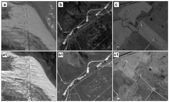
Figure 3.
Example of the shadows produced by the wind plants considering Sentinel (a–c) and CBERS 4A images (a1,b1,c1).
2.1.2. Annotations
The mapping of all wind plants used on-screen visual interpretation by using the CBERS 4A images as reference. Our proposed annotation approach considered the visual interpretation of the wind plant installation considered the following features: (1) foundation concrete, a circular base with a diameter of approximately 20 m; (2) wind turbines and blades that rotate the rotor with the force of the wind; and (3) the shadow areas. One of the most significant difficulties in the computer vision community is dealing with small objects, defined as elements with less than 322 pixels [67,68]. Although wind plants are a prominent object in height, they are not notable in remote sensing orbital images with a nadir view due to their reduced width. We provide an innovative approach by using the shadow features of the wind plants to facilitate its detection [64], which are usually undesirable in most detection problems as they hide the intended objects [69].
2.1.3. Deep Learning Samples
Orbital remote sensing images have extensive dimensions, requiring a subdivision into small patches. This study considered patches with 128 × 128 pixels, suitable for including the wind plant, its shadow, and a good portion of background elements. Each wind plant had at least one 128 × 128 sample, adding at least 20 samples with background-only information. Among the 21 CBERS-4A scenes, 14 were for training, three for validation, three for testing, and one for evaluating the sliding window procedure (Table 1). The final dataset included 4544, 257, and 220 patches for training, validation, and testing, respectively.

Table 1.
Dataset information considering the state, location (latitude and longitude), number of wind plants, number of patches, and the set (train, validation, test, or sliding windows (SW)). The dataset considered the following Brazilian states: Bahia (BA), Ceará (CE), Piauí (PI), Rio Grande do Norte (RN), Rio Grande do Sul (RS), and Rio de Janeiro (RJ).
2.2. Deep Learning Approach
Instance segmentation models such as the Mask-RCNN [70] are the primary approach for recognizing individual objects at a pixel level. However, instance segmentation models for orbital remote sensing may present additional difficulties regarding semantic segmentation: (1) more structured information data requirement (e.g., COCO [68]); (2) increasing object detection parameters (e.g., anchor boxes) and procedures (e.g., ROI alignment); (3) image reconstruction by sliding windows becomes challenging; and (4) worse pixel metrics, especially for small objects. Because the wind farms and their shadows do not touch each other, it is simple to convert semantic features to instance features by using post segmentation methods [71,72]. We used semantic segmentation models to classify all input image pixels [73,74]. The models usually present a structure with contraction (extracting meaningful features) and extension (restoring the image dimension) paths. This study compared five state-of-the-art semantic segmentation architectures: U-Net [75], DeepLabv3+ [76], Feature Pyramid Network (FPN) [77], and U-Net++ [78]. Furthermore, the model evaluation considered three backbones: Efficient-net-B7 [79], ResNeXt-101 [80], and ResNet-101 [81]. The hyperparameters for all models were a learning rate of 0.0001, batch size of 20, and 100 epochs. Moreover, we used random horizontal and vertical flip for avoiding overfitting problems. The image processing used a computer equipped with an NVIDIA RTX 3090 and i9 processor for all experiments.
2.3. Sliding Windows Approach for Classifying Large Areas
The sliding window (SW) approach is commonly used in large-scale image segmentation. This approach involves dividing an image into smaller segments that are equivalent in size to the training samples, with an overlap area defined by the stride value. The stride value is the distance between the centers of the windows and determines the degree of overlap between them. During the classification process, the SW approach classifies the image in sequential frames, starting from the top left corner and moving toward the bottom right corner. The stride value is crucial in semantic segmentation, as it determines the accuracy of the result. A smaller stride value leads to a greater overlap area and better results, as it minimizes errors by averaging overlapping pixels [82,83]. However, it also increases the computational cost. This tradeoff between performance and computational cost is a common challenge when using SW approaches. This study evaluated four stride values (16, 32, 64, and 128) in an independent scene with a high concentration of wind power stations. This investigation helped us determine the optimal stride value that balances accuracy and computational efficiency.
2.4. Semantic to Instance Conversion by Using GIS
This study presents a novel approach to converting semantic to instance segmentation for wind farm monitoring. Our approach leverages the natural distance between wind farms to separate grouped objects, eliminating the need for traditional methods, such as those described in studies [71,72,84], which insert borders to isolate grouped objects. This results in faster and more accurate object counting and reduces the potential for individual recognition errors. Converting to GIS platforms (such as ArcGIS) provides a simple and effective way to handle the data and eliminate noisy predictions by limiting the polygon size, further increasing the accuracy of the results. By considering the shadows and turbines in our annotation strategy and utilizing the 2-m resolution images from the CBERS-4A satellite, the study provides a low-cost solution for monitoring wind plants, reducing the need for technical visits and providing quick and accurate inspection information. To remove noisy predictions, we eliminated polygons with areas below 350 m2 because the wind plants have an average of more than 800 m2.
2.5. Deep Learning Metrics
Most of the accuracy metrics of semantic segmentation models come from the confusion matrix. Because our problem is binary (background or wind plant), there are four possibilities: true positives (TP), true negatives (TN), false positives (FP), and false negatives (FN). In this regard, we assessed five metrics (overall accuracy, precision, recall, F-score, and intersection over union) from the confusion matrix to evaluate the quality of the deep learning models (Table 2).
Table 2.
Accuracy metrics used in this study, in which TP, TN, FP, and FN represent true positives, true negatives, false positives, and false negatives, respectively.
Even though overall accuracy is a straightforward metric, in our scenario, it tends to be less informative because the objects represent a small portion of each image tile, showing a high percentage of true negatives. Precision and recall bring an interesting analysis of the results. However, both are not too informative alone, e.g., if the deep learning model predicts only one pixel as being a wind plant and this pixel is correct, the precision will be 100% and if the model predicts that all pixels are wind plants, the recall will be 100%. The F-score is the harmonic mean between precision and recall, which is much more informative. Finally, the IoU is the primary metric in most competitions because it considers both types of errors (FP and FN) while ignoring the TN. For all metrics, we used a threshold value of 0.5.
To evaluate the sliding windows approach, the ranking metrics that evaluate classifiers over variable thresholds are adequate, so we used precision area-recall under the curve (PR-AUC) and the receiver operating area under the curve (ROC AUC). Finally, we evaluated per-object metrics on the testing image, in which an object with an IoU greater than 0.5 was considered a TP.
3. Results
3.1. Model Evaluation and Comparison
Table 3 lists the results considering the different architectures and backbones. The IoU and F-score are usually the most appropriate in choosing the best model because they consider FP and FN errors. For both IoU and F-score, the best model used the LinkNet architecture with the Eff-B7 backbone, but the U-Net and U-Net++ models presented similar scores. DLv3+ and FPN presented more than a 3% difference in the best models from the other three. Interestingly, only three of the 15 models presented a recall score higher than the precision score. The accuracy analysis proves to be very misleading because most of the pixels are background, and most models presented very high scores near 100%.
Table 3.
Accuracy, precision, recall, F-score, and intersection over union (IoU) metrics for the DeepLabv3+ (DLv3+), U-Net, LinkNet, Feature Pyramid Network (FPN), and U-Net++ architectures and Efficient-net-B7 (Eff-B7), ResNeXt-101 (X-101), and ResNet-101 (R-101) backbones.
Figure 4 shows examples from the test set for the best model (LinkNet with the Eff-B7 backbone). The results demonstrate that the models could understand distinct shadow representations, which is very accurate for mapping wind plants. Nonetheless, there are some spots in which the algorithm may present some errors. Figure 5 shows three examples of possible errors that may occur. The first row shows lookalike features, erroneously detecting a wind plant shadow. The second and third examples show discontinuity errors with relevance in the raster to polygon conversion due to the possibility of giving misleading results.
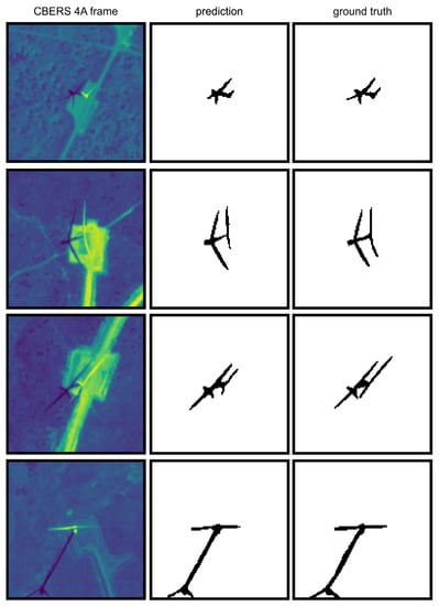
Figure 4.
Image patches from the test set considering the original CBERS 4A image, ground truth, and deep learning prediction.
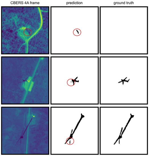
Figure 5.
Image patches from the test set considering the original CBERS 4A image, ground truth, and deep learning prediction. The spots in red are highlighted areas that show in more detail the areas with errors.
Table 4 lists the training period for each model and the inference time on a single 128 × 128 frame. For DeepLabv3+, U-Net, FPN, and LinkNet, the training period for a single epoch presented a similar behavior among the three backbones, in which Eff-B7 > X-101 > R-101. The U-Net++ had a higher training period for X-101 than the rest. Note that the overall behavior tends to be preserved, but changing the computer configurations may vary the results.
Table 4.
Training period (in seconds), and inference time (in milliseconds) considering a computer equipped with an NVIDIA RTX 3090 (24 GB RAM) with an i9 processor for the DeepLabv3+ (DLv3+), U-Net, LinkNet, Feature Pyramid Newtork (FPN), and U-Net++ architectures and the Efficient-net-B7 (Eff-B7), ResNeXt-101 (X-101), and ResNet-101 (R-101) backbones.
3.2. Sliding Window Results
Table 5 lists the results considering different stride values for the ROC AUC and PR-AUC scores. The scene presented 19,968 × 19,968-pixel dimensions, and varying the dimensions would directly affect the mapping time because the number of necessary iterations would change. This scene used a 128-pixel stride, which corresponds to no overlapping pixels, takes nearly 22 min to complete. The required time quickly escalates when reducing the stride. The time nearly quadruplicated when reducing the stride by two. Within those tests, the metrics keep climbing when reducing the strides. However, the improvement tends to get lower each time. Figure 6 shows some differences in predictions with distinct strides. The quality of the data segmentation improves by decreasing the stride, but the main information is knowing where the wind farms are. Thus, the stride choice for practical applications will depend on the types of errors present (such as continuity errors) and the computational resources.
Table 5.
Receiver operation characteristic (ROC AUC), precision-recall area under the curve (PR AUC), intersection over union (IoU), and mapping time using different stride values.
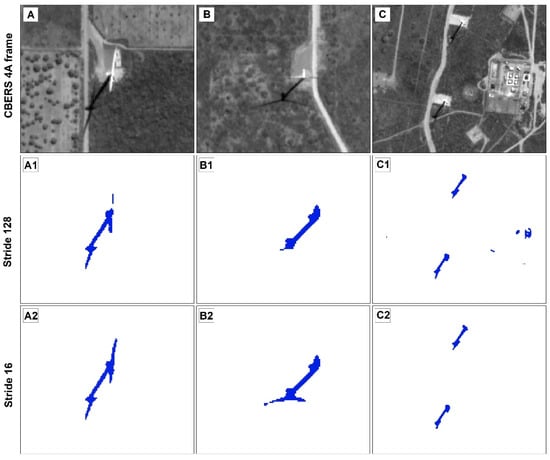
Figure 6.
Differences in the results from the sliding windows approach using different stride values, in which (A–C) are three CBERS-4A images, (A1–C1) are the predictions using a stride of 128, and (A2–C2) are the predictions using a stride of 16.
3.3. Final GIS Representation
Figure 7 shows the final representation with the targets in shapefile format after the raster to polygon operation. Noisy representations are prevalent errors that, in this situation, would bring misleading results because we can estimate the number of wind power plants as the number of polygons. Noisy polygons are predominantly much smaller than those in wind farms. Wind farms average more than 900 m2, and errors are generally less than 350 m2. Thus, elimination using a size threshold value is a viable solution to avoid this type of error. To prove this case, Table 6 lists the per-object results, in which the accuracy is over 90%, showing the efficiency of the overall method. The elimination procedure significantly impacts this kind of analysis because the total number of eliminated noisy features was 1092, which would lower the presented metrics considerably and provide misleading results for inspection and decision-making. Another interesting result is the absence of false negatives, meaning that the deep learning algorithm detected all wind plants. The main errors were the false positives from similar features, including shadows and white objects. Figure 8 shows four examples of false positive errors, in which Figure 8A is an equivalent tower structure, and Figure 8B–D are preliminary constructions in the location of wind plants, which present similar designs and shadows. Some of the errors are difficult even for humans to identify.
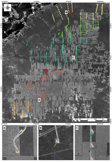
Figure 7.
Results using GIS software, and three zoomed areas (A–C), in which the different colored objects represent different instances from wind plants.
Table 6.
Per-object metrics considering the true positives, false positives, false negatives, and overall accuracy.
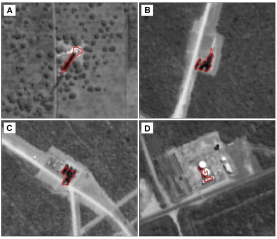
Figure 8.
Four error examples (A–D) in the final classification.
4. Discussion
The discussion is subdivided into the main topics of novelties presented in this study: (Section 4.1) the importance of the application, (Section 4.2) the significance of the proposed data-centric approach, and (Section 4.3) the interpretation and comparison of the deep-learning results.
4.1. Importance of the Application and Dataset
The diversification of the Brazilian energy mix with renewable sources and the establishment of alternatives to hydroelectric plants are fundamental strategies to be in line with the commitment to reduce carbon emissions of the 2030 agenda and minimize the dependence on hydropower, which could bring energy security concerns in case of long periods of drought. In this sense, the expansion of energy production needed to meet future demands will rely on more decentralized and intermittent sources such as wind and solar. The construction of wind farms has increased significantly due to the vast resource of this natural source in the Brazilian territory and government actions to reduce the risk that allows a high power-generation capacity at competitive costs [85,86].
The recent prospect of accelerated growth in wind generation capacity makes it imperative that regulatory agencies invest in technological innovations that quickly satisfy regulatory demands. Technological improvement to obtain continuous inspection of works in progress or under concession is a crucial factor in increasing efficiency and effectiveness given the increasing number of processes, lack of ANEEL employees (particularly for inspection in rural areas), and the high degree of irregularities [22,87]. Therefore, the government and market players must be able to monitor the progress of the construction of new wind farms to guarantee investments and prospection of areas. Developing a technological system based on remote sensing images and deep learning establishes a vital tool and database capable of continuous monitoring that can improve inspection with reduced human work and promote other innovations in spatial analysis. In addition, ongoing surveillance based on free remote sensing data encourages investors to adhere and comply with the regulatory process and allows special attention to be given to disclosing information on investments in wind energy production. Spatial information, constantly updated and available for public consultation, allows the temporal evaluation of investments in infrastructure, favoring investors, community, and public agencies in planning significant decisions in the electricity sector. Therefore, this research establishes an automated pipeline solution for monitoring the construction of wind farms by using remote sensing and deep learning methods, achieving low costs, high frequency, and coverage of large areas.
4.2. Significance of the Data-Centric Approach
This study presented a novel data-centric approach to mapping wind plants by using deep learning. Unlike previous studies that rely solely on points for identifying wind turbines [56,57], our approach leverages semantic segmentation to achieve a more comprehensive target representation. Our approach offers several advantages over traditional point-based methods, as follows.
- Detailed Object Assessment: By using semantic segmentation to delineate the features of wind turbines, we can gather more information about the object, allowing for a broader range of future studies, such as the proper identification of different stages of wind plant construction.
- Consistent Annotation Pattern: Our approach ensures a more consistent pattern in the annotations, leading to more accurate results. Point-based approaches can be unpredictable and reduce the model’s ability to generalize.
- Easy Conversion to Points: Our pipeline includes transforming predictions into vectors, making it easy to convert the segmentation results into points. However, the reverse application is not possible. For example, we have created a point shapefile for each target by using GIS software (Figure 9).
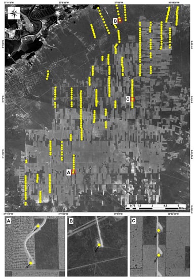 Figure 9. Mapping of the wind plants with three zoomed areas (A–C) considering point shapefile representation.
 - Robust Dataset: Our annotation pattern is more understandable for other researchers and helps increase the robustness of the dataset. Point-based methods can be prone to error, but our approach avoids this problem by considering the entire object.
- Leveraging Shadows: Our approach leverages the shadow cast by wind turbines, which is often an undesired feature, as one of the main features for our annotations. By doing so, we reduce the possibility of predicting noisy features and improve the accuracy of the results.
Moreover, our approach stands out by integrating semantic segmentation and GIS to obtain instance segmentation results, offering a significant advantage over traditional methods. Creating instance segmentation datasets has always been challenging due to the complex annotation format and the demanding sliding window mechanism, which requires precise bounding boxes and instance-level predictions. The proposed method simplifies the process, allowing for a decrease in the stride value to obtain more accurate results but with increased processing time. Additionally, the GIS environment enables noisy feature removal based on the polygon size. In the present case, the elimination of polygons with areas below 350 m2 achieved an accuracy per object of 90%. This noise removal highlights our solution’s efficiency and customization capabilities, making it an effective alternative to traditional methods. Moreover, GIS facilitates the analysis and interpretation of results in polygon and georeferenced format, presenting a more robust ability to understand them on an interactive display.
4.3. Interpretation and Comparison of the Deep Learning Results
This remote sensing application uses deep-learning architectures to detect wind farms by establishing an extensive database containing a wide distribution in tropical scenarios for semantic segmentation. There is great importance in elaborating a new dataset, and this study proposes the first deep-learning dataset for wind energy in the Brazilian territory to be publicly available. Unlike the wind turbine dataset developed by Manso–Callejo et al. [56], which considered high-resolution aerial photography images, the present study developed the first database with orbital images with continuous labels.
This study does not propose any novelties in deep learning architectures. However, we thoroughly analyzed state-of-the-art methods to verify the differences in performance and choose the best model that suits our data. The results of the different CNN models reached a high accuracy, in which the best model was the LinkNet architecture with Eff-B7 backbone. However, the U-Net and U-Net++ models using the Eff-B7 backbone obtained close accuracy metrics. These results show that the choice of the deep learning architecture and backbone is less important than assuring the data quality. In agreement with our results, Han et al. [59] also presented better results for the LinkNet architecture. Our findings differ from Manso-Callejo et al. [57], in which the best result was using the LinkNet with the Eff-B3 backbone, and Manso-Callejo et al. [56], in which the best result was using the LinkNet with the Eff-B2 backbone. It is worth mentioning that none of those studies tested the Efficient-net-B7 backbone. A possible reason is the additional computational resources needed because the Efficient-net-B7 has around 63 million parameters, Efficient-net-B3 has 10 million, and Efficient-net-B0 has four million, showing that some state-of-the-art models require robust computational resources, and their training may not be possible.
5. Conclusions
This research aimed to create a comprehensive pipeline to detect and monitor the construction of wind power plants in the Brazilian territory by using deep learning, remote sensing images with free distribution (CBERS-4A), and GIS technologies. Formulating a low-cost and efficient solution for continuously monitoring the execution of the works is a significant advance for ANEEL, avoiding the survey in the field. The database covered the entire Brazilian territory, offering an extensive resource with several intraregional characteristics applicable to training new models or detecting wind farms in other regions through transfer learning. In addition, the study proposes the following contributions: (a) a new data-centric approach, (b) the use of semantic segmentation and GIS to obtain instance-level predictions, and (c) a new easy-to-replicate annotation pattern. The LinkNet architecture with EfficientNet-B7 backbone obtained the best results among 15 evaluated models. Elaborating large images from deep learning frames (128 × 128 pixels) used the sliding window method with different stride values (16, 32, 64, and 128 pixels) to assess the tradeoff between performance accuracy and computational time. The conversion of semantic segmentation to instance segmentation based on the polygonization of the segments and treatment in a GIS environment allowed a simple identification and counting of the wind power plants and filtering of eventual noises by the polygon size. For future studies, exploring other deep learning architectures and backbones would be beneficial to improve the model’s performance further and consider incorporating other mechanisms, such as incrementing the dataset with more images from different places. Additionally, it would be interesting to examine the scalability of the proposed pipeline in different countries with varying landscapes and wind plant configurations.
Author Contributions
Conceptualization, O.L.F.d.C., O.A.d.C.J., A.G.O. and I.H.; methodology, O.L.F.d.C.; software, O.L.F.d.C.; validation, A.O.d.A.; formal analysis, O.L.F.d.C. and O.A.d.C.J.; investigation, O.L.F.d.C. and A.O.d.A.; resources, O.A.d.C.J., R.A.T.G., A.G.O. and I.H.; data curation, O.L.F.d.C. and A.O.d.A.; writing—original draft preparation, O.L.F.d.C. and O.A.d.C.J.; writing—review and editing, R.F.G., R.A.T.G., D.L.B. and I.H.; visualization, O.L.F.d.C. and A.O.d.A.; supervision, O.A.d.C.J., R.A.T.G., R.F.G. and D.L.B.; project administration, O.L.F.d.C., O.A.d.C.J., A.G.O. and I.H.; funding acquisition, O.A.d.C.J., R.A.T.G. and R.F.G. All authors have read and agreed to the published version of the manuscript.
Funding
This research was funded by the following institutions: National Council for Scientific and Technological Development (434838/2018-7 and 312608/2021-7) and Coordination for the Improvement of Higher Education Personnel (Finance Code 001).
Data Availability Statement
The data that support the findings of this study are available from the corresponding author, upon reasonable request.
Acknowledgments
The authors are grateful for financial support from the CNPq fellowship (Osmar Abílio de Carvalho Júnior, Roberto Arnaldo Trancoso Gomes, and Renato Fontes Guimarães). Special thanks are given to the Laboratory of Spatial Information System research group of the University of Brasilia for technical support. The authors also thank the Brazilian National Electrical Agency (ANEEL), who provided technical support and disposed of crucial data and researchers that helped conduct this project. Finally, the authors acknowledge the contribution of anonymous reviewers.
Conflicts of Interest
The authors declare no conflict of interest.
References
- Lima, M.A.; Mendes, L.F.R.; Mothé, G.A.; Linhares, F.G.; de Castro, M.P.P.; da Silva, M.G.; Sthel, M.S. Renewable energy in reducing greenhouse gas emissions: Reaching the goals of the Paris agreement in Brazil. Environ. Dev. 2020, 33, 100504. [Google Scholar] [CrossRef]
- Tollefson, J. Brazil ratification pushes Paris climate deal one step closer. Nature 2020, 1–2. [Google Scholar] [CrossRef]
- Jiang, X.; Lu, D.; Moran, E.; Calvi, M.F.; Dutra, L.V.; Li, G. Examining impacts of the Belo Monte hydroelectric dam construction on land-cover changes using multitemporal Landsat imagery. Appl. Geogr. 2018, 97, 35–47. [Google Scholar] [CrossRef]
- Mayer, A.; Castro-Diaz, L.; Lopez, M.C.; Leturcq, G.; Moran, E.F. Is hydropower worth it? Exploring amazonian resettlement, human development and environmental costs with the Belo Monte project in Brazil. Energy Res. Soc. Sci. 2021, 78, 102129. [Google Scholar] [CrossRef]
- Gauthier, C.; Lin, Z.; Peter, B.G.; Moran, E.F. Hydroelectric Infrastructure and Potential Groundwater Contamination in the Brazilian Amazon: Altamira and the Belo Monte Dam. Prof. Geogr. 2019, 71, 292–300. [Google Scholar] [CrossRef]
- Gauthier, C.; Moran, E.F. Public policy implementation and basic sanitation issues associated with hydroelectric projects in the Brazilian Amazon: Altamira and the Belo Monte dam. Geoforum 2018, 97, 10–21. [Google Scholar] [CrossRef]
- Castro-Diaz, L.; Lopez, M.C.; Moran, E. Gender-Differentiated Impacts of the Belo Monte Hydroelectric Dam on Downstream Fishers in the Brazilian Amazon. Hum. Ecol. 2018, 46, 411–422. [Google Scholar] [CrossRef]
- Runde, A.; Hallwass, G.; Silvano, R.A.M. Fishers’ Knowledge Indicates Extensive Socioecological Impacts Downstream of Proposed Dams in a Tropical River. One Earth 2020, 2, 255–268. [Google Scholar] [CrossRef]
- Bro, A.S.; Moran, E.; Calvi, M.F. Market participation in the age of big dams: The Belo Monte hydroelectric dam and its impact on rural Agrarian households. Sustainability 2018, 10, 1592. [Google Scholar] [CrossRef]
- Calvi, M.F.; Moran, E.F.; da Silva, R.F.B.; Batistella, M. The construction of the Belo Monte dam in the Brazilian Amazon and its consequences on regional rural labor. Land Use Policy 2020, 90, 104327. [Google Scholar] [CrossRef]
- Ferraz de Andrade Santos, J.A.; de Jong, P.; Alves da Costa, C.; Torres, E.A. Combining wind and solar energy sources: Potential for hybrid power generation in Brazil. Util. Policy 2020, 67, 101084. [Google Scholar] [CrossRef]
- Ministério de Minas e Energia; Empresa de Pesquisa Energética. Plano Decenal de Expansão de Energia 2031; MME/EPE: Brasilia, Brazil, 2022.
- Mendes, L.F.R.; Sthel, M.S. Analysis of the hydrological cycle and its impacts on the sustainability of the electric matrix in the state of Rio de Janeiro/Brazil. Energy Strateg. Rev. 2018, 22, 119–126. [Google Scholar] [CrossRef]
- Hunt., J.D.; Stilpen, D.; de Freitas, M.A.V. A review of the causes, impacts and solutions for electricity supply crises in Brazil. Renew. Sustain. Energy Rev. 2018, 88, 208–222. [Google Scholar] [CrossRef]
- Corrêa Da Silva, R.; De Marchi Neto, I.; Silva Seifert, S. Electricity supply security and the future role of renewable energy sources in Brazil. Renew. Sustain. Energy Rev. 2016, 59, 328–341. [Google Scholar] [CrossRef]
- Mendes, L.F.R.; Sthel, M.S. Thermoelectric Power Plant for Compensation of Hydrological Cycle Change: Environmental Impacts in Brazil. Case Stud. Environ. 2017, 1, 1–7. [Google Scholar] [CrossRef]
- Melo, L.B.; Estanislau, F.B.G.L.; Costa, A.L.; Fortini, Â. Impacts of the hydrological potential change on the energy matrix of the Brazilian State of Minas Gerais: A case study. Renew. Sustain. Energy Rev. 2019, 110, 415–422. [Google Scholar] [CrossRef]
- Reichert, B.; Souza, A.M. Interrelationship simulations among Brazilian electric matrix sources. Electr. Power Syst. Res. 2021, 193, 107019. [Google Scholar] [CrossRef]
- Sampaio, P.G.V.; González, M.O.A. Photovoltaic solar energy: Conceptual framework. Renew. Sustain. Energy Rev. 2017, 74, 590–601. [Google Scholar] [CrossRef]
- de Jong, P.; Barreto, T.B.; Tanajura, C.A.S.; Kouloukoui, D.; Oliveira-Esquerre, K.P.; Kiperstok, A.; Torres, E.A. Estimating the impact of climate change on wind and solar energy in Brazil using a South American regional climate model. Renew. Energy 2019, 141, 390–401. [Google Scholar] [CrossRef]
- Filgueiras, A.; Thelma Maria, T.M.V. Wind energy in Brazil—Present and future. Renew. Sustain. Energy Rev. 2003, 7, 439–451. [Google Scholar] [CrossRef]
- Orlandi, A.G.; Farias, R.A.N.; de Carvalho Junior, O.A.; Guimarães, R.F.; Gomes, R.A.T. Controle gerencial na administração pública e transformação digital: Sensoriamento remoto. Cad. Gestão Pública Cid. 2021, 26, 1–24. [Google Scholar] [CrossRef]
- Bradbury, K.; Saboo, R.; Johnson, T.L.; Malof, J.M.; Devarajan, A.; Zhang, W.; Collins, L.M.; Newell, R.G. Distributed solar photovoltaic array location and extent dataset for remote sensing object identification. Sci. Data 2016, 3, 1–9. [Google Scholar] [CrossRef]
- Jie, Y.; Ji, X.; Yue, A.; Chen, J.; Deng, Y.; Chen, J.; Zhang, Y. Combined Multi-Layer Feature Fusion and Edge Detection Method for Distributed Photovoltaic Power Station Identification. Energies 2020, 13, 6742. [Google Scholar] [CrossRef]
- Zhuang, L.; Zhang, Z.; Wang, L. The automatic segmentation of residential solar panels based on satellite images: A cross learning driven U-Net method. Appl. Soft Comput. J. 2020, 92, 106283. [Google Scholar] [CrossRef]
- Karoui, M.S.; Benhalouche, F.Z.; Deville, Y.; Djerriri, K.; Briottet, X.; Houet, T.; Le Bris, A.; Weber, C. Partial linear NMF-based unmixing methods for detection and area estimation of photovoltaic panels in urban hyperspectral remote sensing data. Remote Sens. 2019, 11, 2164. [Google Scholar] [CrossRef]
- Malof, J.M.; Bradbury, K.; Collins, L.M.; Newell, R.G. Automatic detection of solar photovoltaic arrays in high resolution aerial imagery. Appl. Energy 2016, 183, 229–240. [Google Scholar] [CrossRef]
- Xia, Z.; Li, Y.; Guo, X.; Chen, R. High-resolution mapping of water photovoltaic development in China through satellite imagery. Int. J. Appl. Earth Obs. Geoinf. 2022, 107, 102707. [Google Scholar] [CrossRef]
- da Costa, M.V.C.V.; de Carvalho, O.L.F.; Orlandi, A.G.; Hirata, I.; de Albuquerque, A.O.; de Silva, F.V.; Guimarães, R.F.; Gomes, R.A.T.; de Carvalho Júnior, O.A. Remote Sensing for Monitoring Photovoltaic Solar Plants in Brazil Using Deep Semantic Segmentation. Energies 2021, 14, 2960. [Google Scholar] [CrossRef]
- Zhang, X.; Zeraatpisheh, M.; Rahman, M.M.; Wang, S.; Xu, M. Texture is important in improving the accuracy of mapping photovoltaic power plants: A case study of ningxia autonomous region, china. Remote Sens. 2021, 13, 3909. [Google Scholar] [CrossRef]
- Plakman, V.; Rosier, J.; van Vliet, J. Solar park detection from publicly available satellite imagery. GIScience Remote Sens. 2022, 59, 461–480. [Google Scholar] [CrossRef]
- Masoom, A.; Kosmopoulos, P.; Bansal, A.; Kazadzis, S. Solar energy estimations in india using remote sensing technologies and validation with sun photometers in urban areas. Remote Sens. 2020, 12, 254. [Google Scholar] [CrossRef]
- Kausika, B.; van Sark, W. Calibration and Validation of ArcGIS Solar Radiation Tool for Photovoltaic Potential Determination in the Netherlands. Energies 2021, 14, 1865. [Google Scholar] [CrossRef]
- Yang, D.; Kleissl, J.; Gueymard, C.A.; Pedro, H.T.C.; Coimbra, C.F.M. History and trends in solar irradiance and PV power forecasting: A preliminary assessment and review using text mining. Sol. Energy 2018, 168, 60–101. [Google Scholar] [CrossRef]
- Al Garni, H.Z.; Awasthi, A. Solar PV Power Plants Site Selection. In Advances in Renewable Energies and Power Technologies; Yahyaoui, I., Ed.; Elsevier: Amsterdam, The Netherlands, 2018; Volume 1, pp. 57–75. ISBN 9780128132173. [Google Scholar]
- Gherboudj, I.; Ghedira, H. Assessment of solar energy potential over the United Arab Emirates using remote sensing and weather forecast data. Renew. Sustain. Energy Rev. 2016, 55, 1210–1224. [Google Scholar] [CrossRef]
- Mahtta, R.; Joshi, P.K.; Jindal, A.K. Solar power potential mapping in India using remote sensing inputs and environmental parameters. Renew. Energy 2014, 71, 255–262. [Google Scholar] [CrossRef]
- Polo, J.; Bernardos, A.; Navarro, A.A.; Fernandez-Peruchena, C.M.; Ramírez, L.; Guisado, M.V.; Martínez, S. Solar resources and power potential mapping in Vietnam using satellite-derived and GIS-based information. Energy Convers. Manag. 2015, 98, 348–358. [Google Scholar] [CrossRef]
- Wang, S.; Zhang, L.; Fu, D.; Lu, X.; Wu, T.; Tong, Q. Selecting photovoltaic generation sites in Tibet using remote sensing and geographic analysis. Sol. Energy 2016, 133, 85–93. [Google Scholar] [CrossRef]
- Spyridonidou, S.; Sismani, G.; Loukogeorgaki, E.; Vagiona, D.G.; Ulanovsky, H.; Madar, D. Sustainable Spatial Energy Planning of Large-Scale Wind and PV Farms in Israel: A Collaborative and Participatory Planning Approach. Energies 2021, 14, 551. [Google Scholar] [CrossRef]
- Sánchez-Aparicio, M.; Del Pozo, S.; Martín-Jiménez, J.A.; González-González, E.; Andrés-Anaya, P.; Lagüela, S. Influence of lidar point cloud density in the geometric characterization of rooftops for solar photovoltaic studies in cities. Remote Sens. 2020, 12, 3726. [Google Scholar] [CrossRef]
- Tiwari, A.; Meir, I.A.; Karnieli, A. Object-based image procedures for assessing the solar energy photovoltaic potential of heterogeneous rooftops using airborne LiDAR and orthophoto. Remote Sens. 2020, 12, 223. [Google Scholar] [CrossRef]
- Prieto, I.; Izkara, J.L.; Usobiaga, E. The application of LiDAR data for the solar potential analysis based on urban 3D model. Remote Sens. 2019, 11, 2348. [Google Scholar] [CrossRef]
- Li, Y.; Liu, C. Estimating solar energy potentials on pitched roofs. Energy Build. 2017, 139, 101–107. [Google Scholar] [CrossRef]
- Bauni, V.; Schivo, F.; Capmourteres, V.; Homberg, M. Ecosystem loss assessment following hydroelectric dam flooding: The case of Yacyretá, Argentina. Remote Sens. Appl. Soc. Environ. 2015, 1, 50–60. [Google Scholar] [CrossRef]
- Chen, G.; Powers, R.P.; de Carvalho, L.M.T.; Mora, B. Spatiotemporal patterns of tropical deforestation and forest degradation in response to the operation of the Tucuruí hydroelectricdam in the Amazon basin. Appl. Geogr. 2015, 63, 1–8. [Google Scholar] [CrossRef]
- Feng, L.; Hu, C.; Chen, X.; Zhao, X. Dramatic inundation changes of China’s two largest freshwater lakes linked to the Three Gorges Dam. Environ. Sci. Technol. 2013, 47, 9628–9634. [Google Scholar] [CrossRef] [PubMed]
- Manyari, W.V.; de Carvalho, O.A. Environmental considerations in energy planning for the Amazon region: Downstream effects of dams. Energy Policy 2007, 35, 6526–6534. [Google Scholar] [CrossRef]
- Deng, C.; Wang, S.; Huang, Z.; Tan, Z.; Liu, J. Unmanned aerial vehicles for power line inspection: A cooperative way in platforms and communications. J. Commun. 2014, 9, 687–692. [Google Scholar] [CrossRef]
- Matikainen, L.; Lehtomäki, M.; Ahokas, E.; Hyyppä, J.; Karjalainen, M.; Jaakkola, A.; Kukko, A.; Heinonen, T. Remote sensing methods for power line corridor surveys. ISPRS J. Photogramm. Remote Sens. 2016, 119, 10–31. [Google Scholar] [CrossRef]
- Ahmad, J.; Malik, A.S.; Xia, L.; Ashikin, N. Vegetation encroachment monitoring for transmission lines right-of-ways: A survey. Electr. Power Syst. Res. 2013, 95, 339–352. [Google Scholar] [CrossRef]
- Zhang, R.; Yang, B.; Xiao, W.; Liang, F.; Liu, Y.; Wang, Z. Automatic Extraction of High-Voltage Power Transmission Objects from UAV Lidar Point Clouds. Remote Sens. 2019, 11, 2600. [Google Scholar] [CrossRef]
- Awrangjeb, M. Extraction of Power Line Pylons and Wires Using Airborne LiDAR Data at Different Height Levels. Remote Sens. 2019, 11, 1798. [Google Scholar] [CrossRef]
- Lecun, Y.; Bengio, Y.; Hinton, G. Deep learning. Nature 2015, 521, 436–444. [Google Scholar] [CrossRef]
- Nogueira, K.; Penatti, O.A.B.; dos Santos, J.A. Towards better exploiting convolutional neural networks for remote sensing scene classification. Pattern Recognit. 2017, 61, 539–556. [Google Scholar] [CrossRef]
- Manso-Callejo, M.-A.; Cira, C.-I.; Garrido, R.P.A.; Matesanz, F.J.G. First Dataset of Wind Turbine Data Created at National Level With Deep Learning Techniques From Aerial Orthophotographs With a Spatial Resolution of 0.5 M/Pixel. IEEE J. Sel. Top. Appl. Earth Obs. Remote Sens. 2021, 14, 7968–7980. [Google Scholar] [CrossRef]
- Manso-Callejo, M.-Á.; Cira, C.-I.; Alcarria, R.; Arranz-Justel, J.-J. Optimizing the Recognition and Feature Extraction of Wind Turbines through Hybrid Semantic Segmentation Architectures. Remote Sens. 2020, 12, 3743. [Google Scholar] [CrossRef]
- Schulz, M.; Boughattas, B.; Wendel, F. DetEEktor: Mask R-CNN based neural network for energy plant identification on aerial photographs. Energy AI 2021, 5, 100069. [Google Scholar] [CrossRef]
- Han, M.; Wang, H.; Wang, G.; Liu, Y. Targets Mask U-Net for wind turbines detection in remote sensing images. Int. Arch. Photogramm. Remote Sens. Spat. Inf. Sci. 2018, XLII–3, 475–480. [Google Scholar] [CrossRef]
- Abedini, F.; Bahaghighat, M.; S’hoyan, M. Wind turbine tower detection using feature descriptors and deep learning. Facta Univ.-Ser. Electron. Energ. 2020, 33, 133–153. [Google Scholar] [CrossRef]
- Shihavuddin, A.; Chen, X.; Fedorov, V.; Nymark Christensen, A.; Andre Brogaard Riis, N.; Branner, K.; Bjorholm Dahl, A.; Reinhold Paulsen, R. Wind Turbine Surface Damage Detection by Deep Learning Aided Drone Inspection Analysis. Energies 2019, 12, 676. [Google Scholar] [CrossRef]
- de Carvalho, O.L.F.; dos Santos de Moura, R.; de Albuquerque, A.O.; de Bem, P.P.; Pereira, R.d.C.; Weigang, L.; Borges, D.L.; Guimarães, R.F.; Gomes, R.A.T.; de Carvalho Júnior, O.A. Instance segmentation for governmental inspection of small touristic infrastructure in beach zones using multispectral high-resolution worldview-3 imagery. ISPRS Int. J. Geo-Information 2021, 10, 813. [Google Scholar] [CrossRef]
- Liu, Y.; Sun, P.; Wergeles, N.; Shang, Y. A survey and performance evaluation of deep learning methods for small object detection. Expert Syst. Appl. 2021, 172, 114602. [Google Scholar] [CrossRef]
- Shen, G.; Xu, B.; Jin, Y.; Chen, S.; Zhang, W.; Guo, J.; Liu, H.; Zhang, Y.; Yang, X. Monitoring wind farms occupying grasslands based on remote-sensing data from China’s GF-2 HD satellite—A case study of Jiuquan city, Gansu province, China. Resour. Conserv. Recycl. 2017, 121, 128–136. [Google Scholar] [CrossRef]
- Mandroux, N.; Dagobert, T.; Drouyer, S.; Von Gioi, R.G. Wind Turbine Detection on Sentinel-2 Images. In Proceedings of the 2021 IEEE International Geoscience and Remote Sensing Symposium IGARSS, Brussels, Belgium, 11–16 July 2021; pp. 4888–4891. [Google Scholar]
- Vrabel, J.C.; Stensaas, G.L.; Anderson, C.; Christopherson, J.; Kim, M.; Park, S.; Cantrell, S. System characterization report on the China-Brazil Earth Resources Satellite-4A (CBERS-4A). In System Characterization of Earth Observation Sensors; Ramaseri Chandra, S.N., Ed.; U.S. Geological Survey Open-File Report 2021-1030; U.S. Geological Survey: Reston, VA, USA, 2021; p. 35. [Google Scholar]
- Tong, K.; Wu, Y.; Zhou, F. Recent advances in small object detection based on deep learning: A review. Image Vis. Comput. 2020, 97, 103910. [Google Scholar] [CrossRef]
- Lin, T.-Y.; Maire, M.; Belongie, S.; Hays, J.; Perona, P.; Ramanan, D.; Dollár, P.; Zitnick, C.L. Microsoft COCO: Common Objects in Context. In Proceedings of the Computer Vision—ECCV 2014, Zurich, Switzerland, 6–12 September 2014; Fleet, D., Tomas, P., Schiele, B., Tuytelaars, T., Eds.; Lecture Notes in Computer Science. Springer: Cham, Switzerland, 2014; Volume 8693, pp. 740–755, ISBN 978-3-319-10601-4. [Google Scholar]
- de Carvalho, O.L.F.; de Carvalho Júnior, O.A.; de Silva, C.R.; de Albuquerque, A.O.; Santana, N.C.; Borges, D.L.; Gomes, R.A.T.; Guimarães, R.F. Panoptic Segmentation Meets Remote Sensing. Remote Sens. 2022, 14, 965. [Google Scholar] [CrossRef]
- He, K.; Gkioxari, G.; Dollar, P.; Girshick, R. Mask R-CNN. IEEE Trans. Pattern Anal. Mach. Intell. 2020, 42, 386–397. [Google Scholar] [CrossRef]
- de Carvalho, O.L.F.; Junior, O.A.d.C.; de Albuquerque, A.O.; Santana, N.C.; Guimaraes, R.F.; Gomes, R.A.T.; Borges, D.L. Bounding Box-Free Instance Segmentation Using Semi-Supervised Iterative Learning for Vehicle Detection. IEEE J. Sel. Top. Appl. Earth Obs. Remote Sens. 2022, 15, 3403–3420. [Google Scholar] [CrossRef]
- Mou, L.; Zhu, X.X. Vehicle Instance Segmentation From Aerial Image and Video Using a Multitask Learning Residual Fully Convolutional Network. IEEE Trans. Geosci. Remote Sens. 2018, 56, 6699–6711. [Google Scholar] [CrossRef]
- Garcia-Garcia, A.; Orts-Escolano, S.; Oprea, S.; Villena-Martinez, V.; Garcia-Rodriguez, J. A Review on Deep Learning Techniques Applied to Semantic Segmentation. arXiv 2017, arXiv:1704.06857. [Google Scholar]
- Guo, Y.; Liu, Y.; Oerlemans, A.; Lao, S.; Wu, S.; Lew, M.S. Deep learning for visual understanding: A review. Neurocomputing 2016, 187, 27–48. [Google Scholar] [CrossRef]
- Ronneberger, O.; Fischer, P.; Brox, T. U-Net: Convolutional Networks for Biomedical Image Segmentation. In Lecture Notes in Computer Science (including subseries Lecture Notes in Artificial Intelligence and Lecture Notes in Bioinformatics); Navab, N., Hornegger, J., Wells, W., Frangi, A., Eds.; Springer: Cham, Switzerland, 2015; Volume 9351, pp. 234–241. ISBN 9783319245737. [Google Scholar]
- Chen, L.-C.; Zhu, Y.; Papandreou, G.; Schroff, F.; Adam, H. Encoder-Decoder with Atrous Separable Convolution for Semantic Image Segmentation. In Proceedings of the Computer Vision—ECCV 2018, Munich, Germany, 8–14 September 2018; Ferrari, V., Hebert, M., Sminchisescu, C., Weiss, Y., Eds.; Lecture Notes in Computer Science; Springer: Cham, Switzerland, 2018; Volume 11211, pp. 833–851. [Google Scholar]
- Lin, T.-Y.; Dollar, P.; Girshick, R.; He, K.; Hariharan, B.; Belongie, S. Feature Pyramid Networks for Object Detection. In Proceedings of the 2017 IEEE Conference on Computer Vision and Pattern Recognition (CVPR), Honolulu, HI, USA, 21–26 July 2017; pp. 936–944. [Google Scholar]
- Zhou, Z.; Rahman Siddiquee, M.M.; Tajbakhsh, N.; Liang, J. UNet++: A Nested U-Net Architecture for Medical Image Segmentation. In Miccai; Stoyanov, D., Taylor, Z., Carneiro, G., Syeda-Mahmood, T., Martel, A., Maier-Hein, L., Tavares, J.M.R.S., Bradley, A., Papa, J.P., Belagiannis, V., et al., Eds.; Lecture Notes in Computer Science; Springer International Publishing: Cham, Switzerland, 2018; Volume 11045, pp. 3–11. ISBN 978-3-030-00888-8. [Google Scholar]
- Tan, M.; Le, Q.V. EfficientNet: Rethinking Model Scaling for Convolutional Neural Networks. In Proceedings of the 36th International Conference on Machine Learning, Long Beach, CA, USA, 9–15 June 2019; pp. 6105–6114. [Google Scholar]
- Xie, S.; Girshick, R.; Dollar, P.; Tu, Z.; He, K. Aggregated Residual Transformations for Deep Neural Networks. In Proceedings of the 2017 IEEE Conference on Computer Vision and Pattern Recognition (CVPR), Honolulu, HI, USA, 21–26 July 2017; pp. 5987–5995. [Google Scholar]
- He, K.; Zhang, X.; Ren, S.; Sun, J. Deep Residual Learning for Image Recognition. In Proceedings of the 2016 IEEE Conference on Computer Vision and Pattern Recognition (CVPR), Las Vegas, NV, USA, 27–30 June 2016; Volume 45, pp. 770–778. [Google Scholar]
- da Costa, L.B.; de Carvalho, O.L.F.; de Albuquerque, A.O.; Gomes, R.A.T.; Guimarães, R.F.; de Carvalho Júnior, O.A. Deep semantic segmentation for detecting eucalyptus planted forests in the Brazilian territory using Sentinel-2 imagery. Geocarto Int. 2021, 37, 6538–6550. [Google Scholar] [CrossRef]
- de Albuquerque, A.O.; de Carvalho Júnior, O.A.; de Carvalho, O.L.F.; de Bem, P.P.; Ferreira, P.H.G.; de Moura, R.; Dos, S.; Silva, C.R.; Trancoso Gomes, R.A.; Fontes Guimarães, R. Deep Semantic Segmentation of Center Pivot Irrigation Systems from Remotely Sensed Data. Remote Sens. 2020, 12, 2159. [Google Scholar] [CrossRef]
- de Carvalho, O.L.F.; de Carvalho Junior, O.A.; de Albuquerque, A.O.; Santana, N.C.; Borges, D.L. Rethinking Panoptic Segmentation in Remote Sensing: A Hybrid Approach Using Semantic Segmentation and Non-Learning Methods. IEEE Geosci. Remote Sens. Lett. 2022, 19, 3512105. [Google Scholar] [CrossRef]
- Simas, M.; Pacca, S. Assessing employment in renewable energy technologies: A case study for wind power in Brazil. Renew. Sustain. Energy Rev. 2014, 31, 83–90. [Google Scholar] [CrossRef]
- Rego, E.E.; de Oliveira Ribeiro, C. Successful Brazilian experience for promoting wind energy generation. Electr. J. 2018, 31, 13–17. [Google Scholar] [CrossRef]
- Orlandi, A.G.; De Carvalho Junior, O.A.; Mendonça, R.C.N.; Guimarães, R.F.; Gomes, R.A.T. Regional management and development with free multi-temporal images: The case of hydroelectric power inspection. Rev. Bras. Gestão Desenvolv. Reg. 2022, 18. [Google Scholar] [CrossRef]


Disclaimer/Publisher’s Note: The statements, opinions and data contained in all publications are solely those of the individual author(s) and contributor(s) and not of MDPI and/or the editor(s). MDPI and/or the editor(s) disclaim responsibility for any injury to people or property resulting from any ideas, methods, instructions or products referred to in the content. |
© 2023 by the authors. Licensee MDPI, Basel, Switzerland. This article is an open access article distributed under the terms and conditions of the Creative Commons Attribution (CC BY) license (https://creativecommons.org/licenses/by/4.0/).