Smooth GIoU Loss for Oriented Object Detection in Remote Sensing Images
Abstract
1. Introduction
- (1)
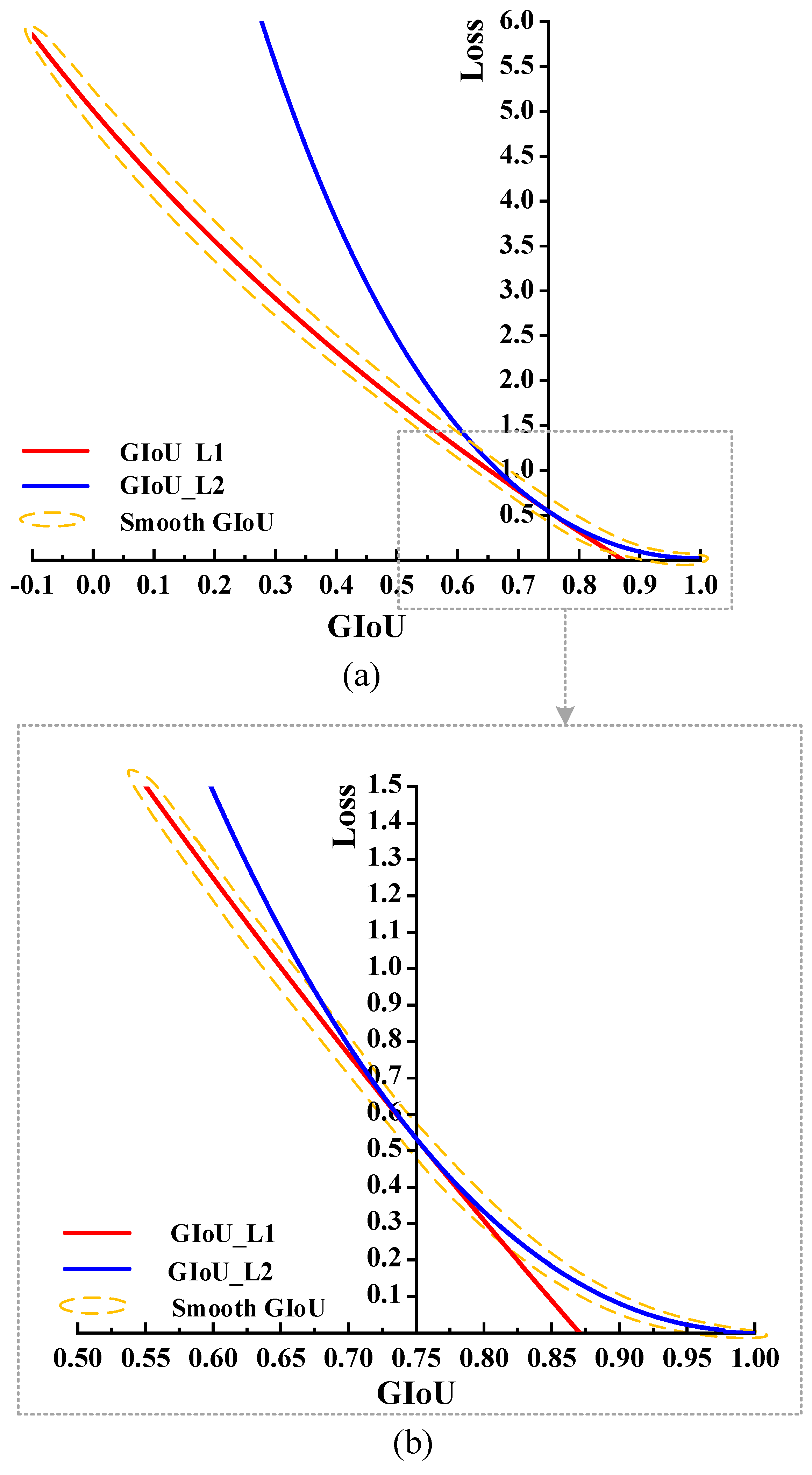
- A novel BBR loss, named smooth GIoU loss, is proposed for OOD in RSIs. The smooth GIoU loss can employ more appropriate learning intensities in the different ranges of the GIoU value. It is worth noting that the design scheme of smooth GIoU loss can be generalized to other IoU-based BBR losses, such as IoU loss [52], DIoU loss [55], EIoU loss [56], etc., regardless of whether it is OOD or HOD.
- (2)
- The existing computational scheme of GIoU is modified to fit OOD.
- (3)
- The experimental results on two RSI datasets demonstrate that the smooth GIoU loss is superior to other BBR losses and has good generalization capability for various kinds of OOD methods.
2. Materials and Methods
2.1. Related Works
2.1.1. Computational Scheme of GIoU for Horizontal Object Detection
2.1.2. Existing GIoU-Based Bounding Box Regression Losses
2.1.3. Other Important Works
2.2. Proposed Method
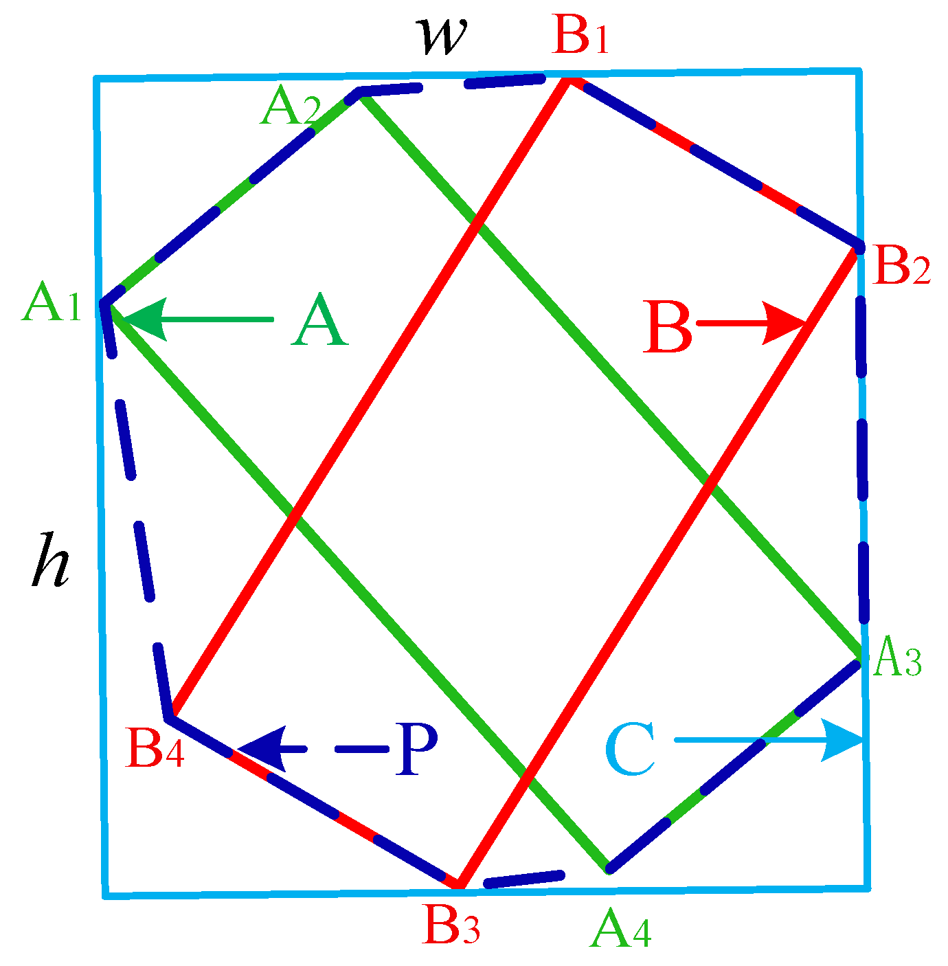
2.2.1. Computational Scheme of GIoU for Oriented Object Detection
| Algorithm 1: Computational scheme of Area(C) |
| Input: Vertex of OBB A:VA = {A1, A2, A3, A4} Vertex of OBB B:VB = {B1, B2, B3, B4} Output: Area(C) 1. Initialize V = ∅ 2. for i = 1 to 4 do 3. if Ai is not enclosed by OBB B then 4. V = append(V, Ai) 5. end if 6. if Bi is not enclosed by OBB A then 7. V = append(V, Bi) 8. end if 9. end for 10. Sort all the vertices in V in a counter/clockwise direction, V = {v1, ,vn}, n ≤ 8. Connect the sorted vertices to obtain P, its n edges is E = {e1,…,en}. 11. for j = 1 to n do 12. for k = 1 to n do 13. d( j, k) = dist_p2l(vj,ek) //smallest distance between vj and ek 14. end for 15. end for 16. w = max d(j, k), 17. (jm, km) = argmax d(j, k), 18. Draw n parallel lines L = {l1, ,ln} through v1∼vn which are all perpendicular to ekm. 19. for j = 1 to n do 20. for k = 1 to n do 21. ld(j, k) = dist_l2l(lj, lk) //distance between lj and lk 22. end for 23. end for 24. h = max ld(j, k), 25. Area(C) = w × h 26. return Area(C) |
2.2.2. Smooth GIoU Loss
Formulation of Smooth GIoU Loss
Proof of the Smooth Characteristic of Smooth GIoU Loss
- (1)
- Proof that GIoU_L1 and GIoU_L2 losses are differentiable:
- (2)
- Proof that GIoU_L1 and GIoU_L2 losses are differentiable and continuous at .
3. Results
3.1. Experimental Setup
3.1.1. Datasets
3.1.2. Implementation Details
3.2. Parameters Analysis
3.3. Comparisons with Other Bounding Box Regression Losses and Ablation Study
3.4. Evaluation of Generalization Capability
3.5. Comprehensive Comparisons
4. Discussion
4.1. Analysis of False Positive Results
- (1)
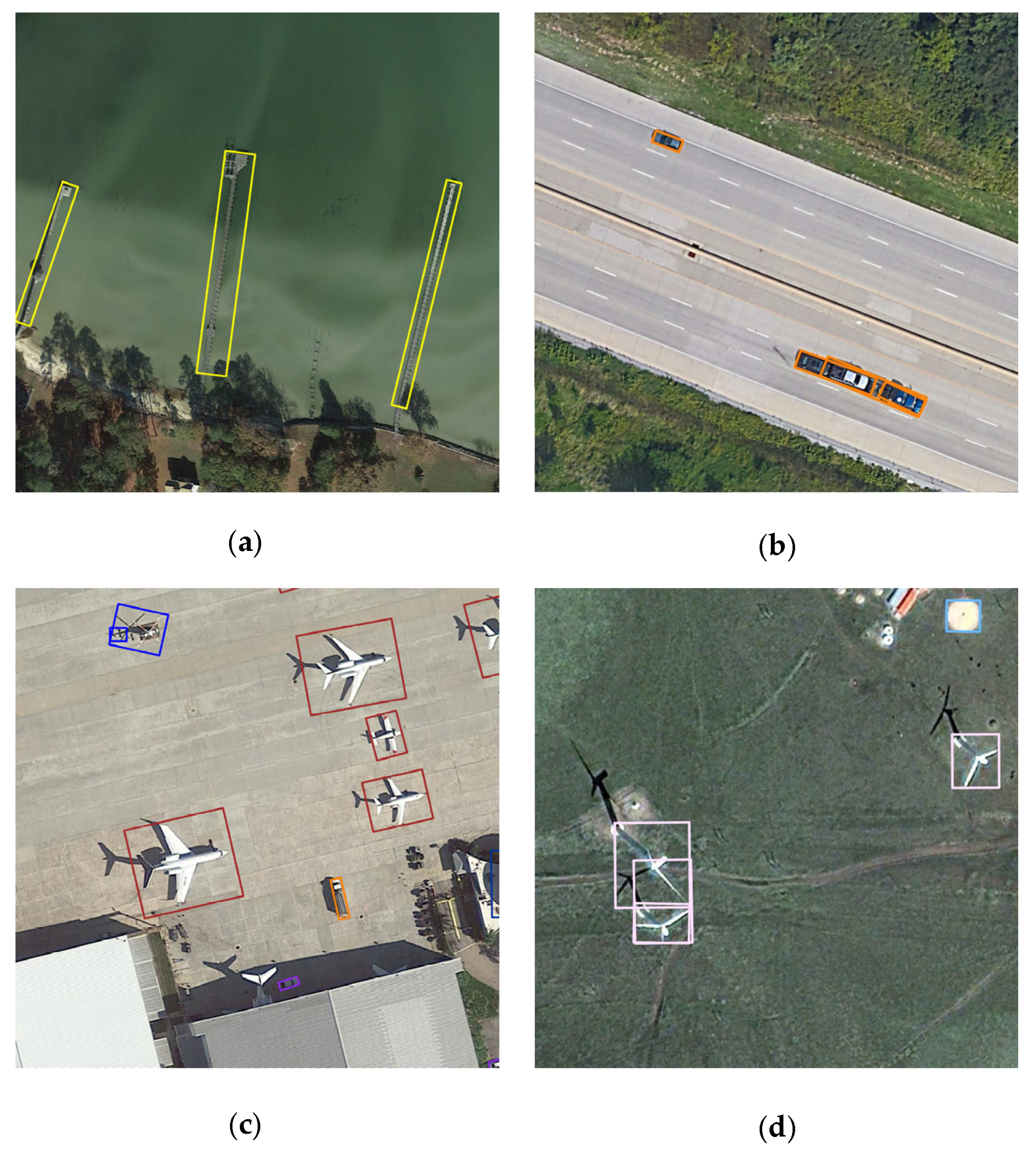
- Similar background. The background regions have similar characteristics to the foreground objects in some cases; consequently, the object detection will be disturbed by the background. As shown in Figure 8a, the harbor has a similar color to the water and trees; therefore, the harbor cannot be completely enclosed by the OBBs.
- (2)
- Dense objects. Foreground objects in the same category are usually similar in appearance; thus, the object detection will be disturbed by adjacent objects in the same category. As shown in Figure 8b, three vehicles are very close to each other and have similar appearances; consequently, two vehicles are enclosed by a single OBB.
- (3)
- Shadow. The shadow of a foreground object usually has similar characteristics to object itself; therefore, the shadow will be falsely identified as the part of object. As shown in Figure 8c,d, the shadows of the helicopter and the windmill are also enclosed by the OBBs.
4.2. Analysis of Running Time and Detection Accuracy after Expanding GPU Memory
5. Conclusions
Author Contributions
Funding
Data Availability Statement
Conflicts of Interest
References
- Yao, X.; Shen, H.; Feng, X.; Cheng, G.; Han, J. R2IPoints: Pursuing Rotation-Insensitive Point Representation for Aerial Object Detection. IEEE Trans. Geosci. Remote Sens. 2022, 60, 1–12. [Google Scholar] [CrossRef]
- Cheng, G.; Cai, L.; Lang, C.; Yao, X.; Chen, J.; Guo, L.; Han, J. SPNet: Siamese-prototype network for few-shot remote sensing image scene classification. IEEE Trans. Geosci. Remote Sens. 2021, 60, 1–11. [Google Scholar] [CrossRef]
- Wu, X.; Hong, D.; Chanussot, J. Convolutional neural networks for multimodal remote sensing data classification. IEEE Trans. Geosci. Remote Sens. 2021, 60, 1–10. [Google Scholar] [CrossRef]
- Hong, D.; Yokoya, N.; Chanussot, J.; Zhu, X.X. An augmented linear mixing model to address spectral variability for hyperspectral unmixing. IEEE Trans. Image Process. 2018, 28, 1923–1938. [Google Scholar] [CrossRef] [PubMed]
- Zhang, L.; Zhang, J.; Wei, W.; Zhang, Y. Learning discriminative compact representation for hyperspectral imagery classification. IEEE Trans. Geosci. Remote Sens. 2019, 57, 8276–8289. [Google Scholar] [CrossRef]
- Cheng, G.; Han, J.; Zhou, P.; Xu, D. Learning rotation-invariant and fisher discriminative convolutional neural networks for object detection. IEEE Trans. Image Process. 2018, 28, 265–278. [Google Scholar] [CrossRef]
- Zhu, Q.; Guo, X.; Deng, W.; Guan, Q.; Zhong, Y.; Zhang, L.; Li, D. Land-use/land-cover change detection based on a Siamese global learning framework for high spatial resolution remote sensing imagery. ISPRS J. Photogramm. Remote Sens. 2022, 184, 63–78. [Google Scholar] [CrossRef]
- Hong, D.; Gao, L.; Yao, J.; Zhang, B.; Plaza, A.; Chanussot, J. Graph convolutional networks for hyperspectral image classification. IEEE Trans. Geosci. Remote Sens. 2020, 59, 5966–5978. [Google Scholar] [CrossRef]
- Wu, X.; Hong, D.; Chanussot, J. UIU-Net: U-Net in U-Net for Infrared Small Object Detection. IEEE Trans. Image Process. 2022, 32, 364–376. [Google Scholar] [CrossRef]
- Hong, D.; Gao, L.; Yokoya, N.; Yao, J.; Chanussot, J.; Du, Q.; Zhang, B. More diverse means better: Multimodal deep learning meets remote-sensing imagery classification. IEEE Trans. Geosci. Remote Sens. 2020, 59, 4340–4354. [Google Scholar] [CrossRef]
- Zhang, L.; Zhang, Y.; Yan, H.; Gao, Y.; Wei, W. Salient object detection in hyperspectral imagery using multi-scale spectral-spatial gradient. Neurocomputing 2018, 291, 215–225. [Google Scholar] [CrossRef]
- Liao, W.; Bellens, R.; Pizurica, A.; Philips, W.; Pi, Y. Classification of hyperspectral data over urban areas using directional morphological profiles and semi-supervised feature extraction. IEEE J. Sel. Top. Appl. Earth Obs. Remote Sens. 2012, 5, 1177–1190. [Google Scholar] [CrossRef]
- Gao, L.; Zhao, B.; Jia, X.; Liao, W.; Zhang, B. Optimized kernel minimum noise fraction transformation for hyperspectral image classification. Remote Sens. 2017, 9, 548. [Google Scholar] [CrossRef]
- Du, L.; You, X.; Li, K.; Meng, L.; Cheng, G.; Xiong, L.; Wang, G. Multi-modal deep learning for landform recognition. ISPRS J. Photogramm. Remote Sens. 2019, 158, 63–75. [Google Scholar] [CrossRef]
- Zhang, L.; Shi, Z.; Wu, J. A hierarchical oil tank detector with deep surrounding features for high-resolution optical satellite imagery. IEEE J. Sel. Top. Appl. Earth Obs. Remote Sens. 2015, 8, 4895–4909. [Google Scholar] [CrossRef]
- Stankov, K.; He, D.-C. Detection of buildings in multispectral very high spatial resolution images using the percentage occupancy hit-or-miss transform. IEEE J. Sel. Top. Appl. Earth Obs. Remote Sens. 2014, 7, 4069–4080. [Google Scholar] [CrossRef]
- Han, X.; Zhong, Y.; Zhang, L. An efficient and robust integrated geospatial object detection framework for high spatial resolution remote sensing imagery. Remote Sens. 2017, 9, 666. [Google Scholar] [CrossRef]
- Qian, X.; Zeng, Y.; Wang, W.; Zhang, Q. Co-saliency Detection Guided by Group Weakly Supervised Learning. IEEE Trans. Multimed. 2022. [CrossRef]
- Qian, X.; Huo, Y.; Cheng, G.; Yao, X.; Li, K.; Ren, H.; Wang, W. Incorporating the Completeness and Difficulty of Proposals Into Weakly Supervised Object Detection in Remote Sensing Images. IEEE J. Sel. Top. Appl. Earth Obs. Remote Sens. 2022, 15, 1902–1911. [Google Scholar] [CrossRef]
- Qian, X.; Li, J.; Cao, J.; Wu, Y.; Wang, W. Micro-cracks detection of solar cells surface via combining short-term and long-term deep features. Neural Netw. 2020, 127, 132–140. [Google Scholar] [CrossRef]
- Zhu, Q.; Deng, W.; Zheng, Z.; Zhong, Y.; Guan, Q.; Lin, W.; Zhang, L.; Li, D. A spectral-spatial-dependent global learning framework for insufficient and imbalanced hyperspectral image classification. IEEE Trans. Cybern. 2021, 52, 11709–11723. [Google Scholar] [CrossRef] [PubMed]
- Zhang, D.; Meng, D.; Han, J. Co-saliency detection via a self-paced multiple-instance learning framework. IEEE Trans. Pattern Anal. Mach. Intell. 2016, 39, 865–878. [Google Scholar] [CrossRef] [PubMed]
- Han, J.; Zhang, D.; Hu, X.; Guo, L.; Ren, J.; Wu, F. Background prior-based salient object detection via deep reconstruction residual. IEEE Trans. Circuits Syst. Video Technol. 2014, 25, 1309–1321. [Google Scholar] [CrossRef]
- Han, J.; Yao, X.; Cheng, G.; Feng, X.; Xu, D. P-CNN: Part-based convolutional neural networks for fine-grained visual categorization. IEEE Trans. Pattern Anal. Mach. Intell. 2019, 44, 579–590. [Google Scholar] [CrossRef] [PubMed]
- Han, J.; Ji, X.; Hu, X.; Zhu, D.; Li, K.; Jiang, X.; Cui, G.; Guo, L.; Liu, T. Representing and retrieving video shots in human-centric brain imaging space. IEEE Trans. Image Process. 2013, 22, 2723–2736. [Google Scholar] [CrossRef]
- Redmon, J.; Farhadi, A. YOLO9000: Better, faster, stronger. In Proceedings of the IEEE Conference on Computer Vision and Pattern Recognition, Honolulu, HI, USA, 21–26 July 2017; pp. 7263–7271. [Google Scholar] [CrossRef]
- Redmon, J.; Farhadi, A. Yolov3: An incremental improvement. arXiv 2018, arXiv:1804.02767. [Google Scholar]
- Liu, W.; Anguelov, D.; Erhan, D.; Szegedy, C.; Reed, S.; Fu, C.-Y.; Berg, A.C. Ssd: Single shot multibox detector. In European Conference on Computer Vision; Springer International Publishing: Berlin/Heidelberg, Germany, 2016; pp. 21–37. [Google Scholar]
- Liu, W.; Ma, L.; Wang, J. Detection of multiclass objects in optical remote sensing images. IEEE Geosci. Remote Sens. Lett. 2018, 16, 791–795. [Google Scholar] [CrossRef]
- Chen, S.; Zhan, R.; Zhang, J. Geospatial object detection in remote sensing imagery based on multiscale single-shot detector with activated semantics. Remote Sens. 2018, 10, 820. [Google Scholar] [CrossRef]
- Tang, T.; Zhou, S.; Deng, Z.; Lei, L.; Zou, H. Arbitrary-oriented vehicle detection in aerial imagery with single convolutional neural networks. Remote Sens. 2017, 9, 1170. [Google Scholar] [CrossRef]
- Tayara, H.; Chong, K.T. Object detection in very high-resolution aerial images using one-stage densely connected feature pyramid network. Sensors 2018, 18, 3341. [Google Scholar] [CrossRef]
- Chen, Z.; Zhang, T.; Ouyang, C. End-to-end airplane detection using transfer learning in remote sensing images. Remote Sens. 2018, 10, 139. [Google Scholar] [CrossRef]
- Ren, S.; He, K.; Girshick, R.; Sun, J. Faster r-cnn: Towards real-time object detection with region proposal networks. Adv. Neural Inf. Process. Syst. 2015, 28, 91–99. [Google Scholar] [CrossRef]
- Dai, J.; Li, Y.; He, K.; Sun, J. R-fcn: Object detection via region-based fully convolutional networks. Adv. Neural Inf. Process. Syst. 2016, 29, 379–387. [Google Scholar]
- Lin, T.-Y.; Dollár, P.; Girshick, R.; He, K.; Hariharan, B.; Belongie, S. Feature pyramid networks for object detection. In Proceedings of the IEEE Conference on Computer Vision and Pattern Recognition, Honolulu, HI, USA, 21–26 July 2017; pp. 2117–2125. [Google Scholar]
- Li, K.; Cheng, G.; Bu, S.; You, X. Rotation-insensitive and context-augmented object detection in remote sensing images. IEEE Trans. Geosci. Remote Sens. 2017, 56, 2337–2348. [Google Scholar] [CrossRef]
- Zhong, Y.; Han, X.; Zhang, L. Multi-class geospatial object detection based on a position-sensitive balancing framework for high spatial resolution remote sensing imagery. ISPRS J. Photogramm. Remote Sens. 2018, 138, 281–294. [Google Scholar] [CrossRef]
- Chen, C.; Gong, W.; Chen, Y.; Li, W. Object detection in remote sensing images based on a scene-contextual feature pyramid network. Remote Sens. 2019, 11, 339. [Google Scholar] [CrossRef]
- Lin, T.-Y.; Goyal, P.; Girshick, R.; He, K.; Dollár, P. Focal loss for dense object detection. In Proceedings of the IEEE International Conference on Computer Vision, Venice, Italy, 22–29 October 2017; pp. 2980–2988. [Google Scholar] [CrossRef]
- Han, J.; Ding, J.; Li, J.; Xia, G.-S. Align deep features for oriented object detection. IEEE Trans. Geosci. Remote Sens. 2021, 60, 1–11. [Google Scholar] [CrossRef]
- Ming, Q.; Zhou, Z.; Miao, L.; Zhang, H.; Li, L. Dynamic anchor learning for arbitrary-oriented object detection. In Proceedings of the AAAI Conference on Artificial Intelligence, Vancouver, BC, Canada, 2–9 February 2021; Volume 35, pp. 2355–2363. [Google Scholar] [CrossRef]
- Zhang, H.; Chang, H.; Ma, B. Dynamic R-CNN: Towards high quality object detection via dynamic training. In Proceedings of the Computer Vision–ECCV 2020: 16th European Conference, Glasgow, UK, 23–28 August 2020. [Google Scholar]
- Li, W.; Chen, Y.; Hu, K. Oriented reppoints for aerial object detection. In Proceedings of the IEEE/CVF Conference on Computer Vision and Pattern Recognition, New Orleans, LA, USA, 18–24 June 2022. [Google Scholar]
- Xia, G.-S.; Bai, X.; Ding, J. DOTA: A large-scale dataset for object detection in aerial images. In Proceedings of the IEEE Conference on Computer Vision and Pattern Recognition, Salt Lake City, UT, USA, 18–22 June 2018. [Google Scholar]
- Mehta, R.; Ozturk, C. Object detection at 200 frames per second. In Proceedings of the European Conference on Computer Vision (ECCV) Workshops; Springer: Berlin/Heidelberg, Germany, 2018. [Google Scholar]
- Zhou, X.; Koltun, V.; Krähenbühl, P. Probabilistic two-stage detection. arXiv 2021, arXiv:2103.07461. [Google Scholar]
- Ma, J.; Shao, W.; Ye, H.; Wang, L.; Wang, H.; Zheng, Y.; Xue, X. Arbitrary-oriented scene text detection via rotation proposals. IEEE Trans. Multimed. 2018, 20, 3111–3122. [Google Scholar] [CrossRef]
- Ding, J.; Xue, N.; Long, Y. Learning roi transformer for oriented object detection in aerial images. In Proceedings of the IEEE/CVF Conference on Computer Vision and Pattern Recognition, Long Beach, CA, USA, 15–20 June 2019; pp. 2849–2858. [Google Scholar]
- Xie, X.; Cheng, G.; Wang, J. Oriented R-CNN for object detection. In Proceedings of the IEEE/CVF International Conference on Computer Vision, Montreal, QC, Canada, 10–17 October 2021. [Google Scholar]
- Girshick, R. Fast r-cnn. In Proceedings of the IEEE International Conference on Computer Vision, Santiago, Chile, 7–13 December 2015. [Google Scholar]
- Zhou, D.; Fang, J.; Song, X.; Guan, C.; Yin, J.; Dai, Y.; Yang, R. Iou loss for 2d/3d object detection. In Proceedings of the 2019 International Conference on 3D Vision (3DV), Québec City, QC, Canada, 16–19 September 2019. [Google Scholar]
- Chen, Z.; Chen, K.; Lin, W. Piou loss: Towards accurate oriented object detection in complex environments. In Proceedings of the European Conference on Computer Vision, Glasgow, UK, 23–28 August 2020. [Google Scholar]
- Rezatofighi, H.; Tsoi, N.; Gwak, J. Generalized intersection over union: A metric and a loss for bounding box regression. In Proceedings of the IEEE/CVF Conference on Computer Vision and Pattern Recognition, Long Beach, CA, USA, 15–20 June 2019. [Google Scholar]
- Zheng, Z.; Wang, P.; Liu, W. Distance-IoU loss: Faster and better learning for bounding box regression. In Proceedings of the AAAI Conference on Artificial Intelligence, New York, NY, USA, 7–12 February 2020. [Google Scholar]
- Zhang, Y.-F.; Ren, W.; Zhang, Z. Focal and efficient IOU loss for accurate bounding box regression. Neurocomputing 2022, 506, 146–157. [Google Scholar] [CrossRef]
- Qian, X.; Lin, S.; Cheng, G. Object detection in remote sensing images based on improved bounding box regression and multi-level features fusion. Remote Sens. 2020, 12, 143. [Google Scholar] [CrossRef]
- Ming, Q.; Miao, L.; Zhou, Z. CFC-Net: A critical feature capturing network for arbitrary-oriented object detection in remote-sensing images. IEEE Trans. Geosci. Remote Sens. 2021, 60, 1–14. [Google Scholar] [CrossRef]
- Pan, X.; Ren, Y.; Sheng, K. Dynamic refinement network for oriented and densely packed object detection. In Proceedings of the IEEE/CVF Conference on Computer Vision and Pattern Recognition, Seattle, WA, USA, 13–19 June 2020. [Google Scholar]
- Zhang, F.; Wang, X.; Zhou, S. DARDet: A dense anchor-free rotated object detector in aerial images. IEEE Geosci. Remote Sens. Lett. 2021, 19, 1–5. [Google Scholar] [CrossRef]
- Wei, Z.; Liang, D.; Zhang, D. Learning calibrated-guidance for object detection in aerial images. IEEE J. Sel. Top. Appl. Earth Obs. Remote Sens. 2022, 15, 2721–2733. [Google Scholar] [CrossRef]
- Tian, Z.; Chu, X.; Wang, X.; Wei, X.; Shen, C. Fully Convolutional One-Stage 3D Object Detection on LiDAR Range Images. arXiv 2022, arXiv:2205.13764. [Google Scholar]
- Wu, Y.; Chen, Y.; Yuan, L. Rethinking classification and localization for object detection. In Proceedings of the IEEE/CVF Conference on Computer Vision and Pattern Recognition, Seattle, WA, USA, 13–19 June 2020. [Google Scholar]
- Cheng, G.; Wang, J.; Li, K. Anchor-free oriented proposal generator for object detection. IEEE Trans. Geosci. Remote Sens. 2022, 60, 1–11. [Google Scholar] [CrossRef]
- Xu, Y.; Fu, M.; Wang, Q. Gliding vertex on the horizontal bounding box for multi-oriented object detection. IEEE Trans. Pattern Anal. Mach. Intell. 2020, 43, 1452–1459. [Google Scholar] [CrossRef]
- Cheng, G.; Yao, Y.; Li, S. Dual-aligned oriented detector. IEEE Trans. Geosci. Remote Sens. 2022, 60, 1–11. [Google Scholar] [CrossRef]
- Yu, D.; Ji, S. A new spatial-oriented object detection framework for remote sensing images. IEEE Trans. Geosci. Remote Sens. 2021, 60, 1–16. [Google Scholar] [CrossRef]
- Han, J.; Ding, J.; Xue, N. Redet: A rotation-equivariant detector for aerial object detection. In Proceedings of the IEEE/CVF Conference on Computer Vision and Pattern Recognition, Nashville, TN, USA, 20–25 June 202.
- Wang, J.; Yang, W.; Li, H.-C. Learning center probability map for detecting objects in aerial images. IEEE Trans. Geosci. Remote Sens. 2020, 59, 4307–4323. [Google Scholar] [CrossRef]
- Shamsolmoali, P.; Chanussot, J.; Zareapoor, M. Multipatch feature pyramid network for weakly supervised object detection in optical remote sensing images. IEEE Trans. Geosci. Remote Sens. 2021, 60, 1–13. [Google Scholar] [CrossRef]
- Miao, S.; Cheng, G.; Li, Q. Precise Vertex Regression and Feature Decoupling for Oriented Object Detection. In Proceedings of the IGARSS 2022-2022 IEEE International Geoscience and Remote Sensing Symposium, Kuala Lumpur, Malaysia, 17–22 July 2022. [Google Scholar] [CrossRef]
- Li, Q.; Cheng, G.; Miao, S. Dynamic Proposal Generation for Oriented Object Detection in Aerial Images. IGARSS 2022-2022 IEEE International Geoscience and Remote Sensing Symposium. In Proceedings of the IGARSS 2022-2022 IEEE International Geoscience and Remote Sensing Symposium, Kuala Lumpur, Malaysia, 17–22 July 2022. [Google Scholar]
- Yao, Y.; Cheng, G.; Wang, G. On Improving Bounding Box Representations for Oriented Object Detection. IEEE Trans. Geosci. Remote Sens. 2022. [Google Scholar] [CrossRef]
- Everingham, M.; Van Gool, L.; Williams, C.K. The pascal visual object classes (voc) challenge. Int. J. Comput. Vis. 2010, 88, 303–338. [Google Scholar] [CrossRef]
- Chen, K.; Wang, J.; Pang, J.; Cao, Y.; Xiong, Y.; Li, X.; Sun, S.; Feng, W.; Liu, Z.; Xu, J. MMDetection: Open mmlab detection toolbox and benchmark. arXiv 2019, arXiv:1906.07155. [Google Scholar]
- Shafiq, M.; Gu, Z. Deep residual learning for image recognition: A survey. Appl. Sci. 2022, 12, 8972. [Google Scholar] [CrossRef]
- Li, Z.; Wang, W.; Li, H. Bevformer: Learning bird’s-eye-view representation from multi-camera images via spatiotemporal transformers. In Proceedings of the Computer Vision–ECCV 2022: 17th European Conference, Tel Aviv, Israel, 23–27 October 2022. [Google Scholar]
| Method | Epoch | Backbone | Loss | mAP | |
|---|---|---|---|---|---|
| DOTA | DIOR-R | ||||
| S2ANet [41] | 12 | R-50-FPN | PIoU Loss | 72.42 | 60.02 |
| Smooth L1 Loss | 74.12 | 62.90 | |||
| IoU Loss | 74.64 | 62.94 | |||
| Smooth IoU Loss | 75.69 | 63.47 | |||
| GIoU Loss | 74.80 | 62.99 | |||
| Baseline GIoU loss | 74.12 | 62.58 | |||
| GIoU_L1 Loss | 74.42 | 62.78 | |||
| GIoU_L2 Loss | 74.93 | 63.13 | |||
| Smooth GIoU Loss | 75.87 | 63.90 | |||
| Methods | Backbone | Epoch | Smooth GIoU Loss | mAP | |
|---|---|---|---|---|---|
| DOTA | DIOR-R | ||||
| RoI Transformer ☨ [49] | R-50-FPN | 12 | √ | 74.61 76.30 (+1.69) | 63.87 64.84 (+0.97) |
| AOPG [64] | √ | 75.24 76.19 (+0.95) | 64.41 66.51 (+2.10) | ||
| Oriented RCNN [50] | √ | 75.87 76.49 (+0.62) | 64.63 65.09 (+0.46) | ||
| S2ANet [41] | √ | 74.12 75.87 (+1.75) | 62.90 63.90 (+1.00) | ||
| RetinaNet-O ☨ [40] | √ | 68.43 69.23 (+0.80) | 57.55 57.89 (+0.34) | ||
| Gliding Vertex [65] | √ | 75.02 75.37 (+0.35) | 60.06 61.02 (+0.96) | ||
| Methods | Backbone | Epoch | PL | BD | BR | GTF | SV | LV | SH | TC |
| One-stage: | ||||||||||
| PIoU [53] | DLA-34 [36] | 12 | 80.90 | 69.70 | 24.10 | 60.20 | 38.30 | 64.40 | 64.80 | 90.90 |
| RetinaNet-O ☨ [40] | R-50-FPN | 12 | 88.67 | 77.62 | 41.81 | 58.17 | 74.58 | 71.64 | 79.11 | 90.29 |
| DRN [59] | H-104 [45] | 120 | 88.91 | 80.22 | 43.52 | 63.35 | 73.48 | 70.69 | 84.94 | 90.14 |
| DAL [42] | R-50-FPN | 12 | 88.68 | 76.55 | 45.08 | 66.80 | 67.00 | 76.76 | 79.74 | 90.84 |
| CFC-Net [58] | R-50-FPN | 25 | 89.08 | 80.41 | 52.41 | 70.02 | 76.28 | 78.11 | 87.21 | 90.89 |
| S2ANet [41] | R-50-FPN | 12 | 89.11 | 82.84 | 48.37 | 71.11 | 78.11 | 78.39 | 87.25 | 90.83 |
| Oriented RepPoints [44] | R-50-FPN | 40 | 87.02 | 83.17 | 54.13 | 71.16 | 80.18 | 78.40 | 87.28 | 90.90 |
| Ours: | ||||||||||
| S2ANet + SmoothGIoU | R-50-FPN | 12 | 89.36 | 81.95 | 53.40 | 74.60 | 78.03 | 81.50 | 87.58 | 90.90 |
| S2ANet + SmoothGIoU | R-50-FPN | 36 | 88.78 | 80.15 | 53.88 | 73.57 | 79.25 | 82.14 | 87.87 | 90.87 |
| S2ANet + SmoothGIoU * | R-50-FPN | 12 | 90.08 | 83.99 | 58.28 | 80.92 | 79.67 | 83.32 | 88.15 | 90.87 |
| S2ANet + SmoothGIoU * | R-50-FPN | 36 | 89.91 | 84.97 | 59.50 | 81.24 | 78.93 | 85.26 | 88.70 | 90.90 |
| Two-stage: | ||||||||||
| Faster R-CNN ☨ [34] | R-50-FPN | 12 | 88.44 | 73.06 | 44.86 | 59.09 | 73.25 | 71.49 | 77.11 | 90.84 |
| CenterMap-Net [69] | R-50-FPN | 12 | 88.88 | 81.24 | 53.15 | 60.65 | 78.62 | 66.55 | 78.10 | 88.83 |
| PVR-FD [71] | R-50-FPN | 12 | 88.70 | 82.20 | 50.10 | 70.40 | 78.70 | 74.20 | 86.20 | 90.80 |
| DPGN [72] | R-101-FPN | 12 | 89.15 | 79.57 | 51.26 | 77.61 | 76.29 | 81.67 | 79.95 | 90.90 |
| RoI Transformer ☨ [49] | R-50-FPN | 12 | 88.65 | 82.60 | 52.53 | 70.87 | 77.93 | 76.67 | 86.87 | 90.71 |
| AOPG [64] | R-50-FPN | 12 | 89.27 | 83.49 | 52.50 | 69.97 | 73.51 | 82.31 | 87.95 | 90.89 |
| DODet [66] | R-50-FPN | 12 | 89.34 | 84.31 | 51.39 | 71.04 | 79.04 | 82.86 | 88.15 | 90.90 |
| Oriented R-CNN [50] | R-50-FPN | 12 | 89.46 | 82.12 | 54.78 | 70.86 | 78.93 | 83.00 | 88.20 | 90.90 |
| Ours: | ||||||||||
| AOPG + Smooth GIoU | R-50-FPN | 12 | 89.62 | 82.89 | 52.24 | 72.34 | 78.27 | 83.08 | 88.18 | 90.89 |
| AOPG + Smooth GIoU | R-50-FPN | 36 | 88.93 | 83.87 | 55.04 | 70.61 | 78.76 | 84.40 | 88.21 | 90.87 |
| AOPG + Smooth GIoU * | R-50-FPN | 12 | 90.25 | 84.80 | 59.46 | 79.80 | 78.99 | 85.15 | 88.56 | 90.90 |
| AOPG + Smooth GIoU * | R-50-FPN | 36 | 89.77 | 85.40 | 59.29 | 79.16 | 79.04 | 84.78 | 88.62 | 90.90 |
| Methods | Backbone | Epoch | BC | ST | SBF | RA | HA | SP | HC | mAP |
| One-stage: | ||||||||||
| PIoU [53] | DLA-34 [36] | 12 | 77.20 | 70.40 | 46.50 | 37.10 | 57.10 | 61.90 | 64.00 | 60.50 |
| RetinaNet-O ☨ [40] | R-50-FPN | 12 | 82.18 | 74.32 | 54.75 | 60.60 | 62.57 | 69.57 | 60.64 | 68.43 |
| DRN [59] | H-104 [45] | 120 | 83.85 | 84.11 | 50.12 | 58.41 | 67.62 | 68.60 | 52.50 | 70.70 |
| DAL [46] | R-50-FPN | 12 | 79.54 | 78.45 | 57.71 | 62.27 | 69.05 | 73.14 | 60.11 | 71.44 |
| CFC-Net [58] | R-50-FPN | 25 | 84.47 | 85.64 | 60.51 | 61.52 | 67.82 | 68.02 | 50.09 | 73.50 |
| S2ANet [41] | R-50-FPN | 12 | 84.90 | 85.64 | 60.36 | 62.60 | 65.26 | 69.13 | 57.94 | 74.12 |
| Oriented RepPoints [44] | R-50-FPN | 40 | 85.97 | 86.25 | 59.90 | 70.49 | 73.53 | 72.27 | 58.97 | 75.97 |
| Ours: | ||||||||||
| S2ANet + SmoothGIoU | R-50-FPN | 12 | 85.08 | 84.59 | 63.23 | 64.84 | 73.62 | 69.25 | 60.06 | 75.87 |
| S2ANet + SmoothGIoU | R-50-FPN | 36 | 85.17 | 84.43 | 62.76 | 70.08 | 75.59 | 71.85 | 56.53 | 76.19 |
| S2ANet + SmoothGIoU * | R-50-FPN | 12 | 84.52 | 87.16 | 72.33 | 72.08 | 80.77 | 80.71 | 65.21 | 79.87 |
| S2ANet + SmoothGIoU * | R-50-FPN | 36 | 88.19 | 87.69 | 70.13 | 69.24 | 82.54 | 78.24 | 73.71 | 80.61 |
| Two-stage: | ||||||||||
| Faster R-CNN ☨ [34] | R-50-FPN | 12 | 78.94 | 83.90 | 48.59 | 62.95 | 62.18 | 64.91 | 56.18 | 69.05 |
| CenterMap-Net [69] | R-50-FPN | 12 | 77.80 | 83.61 | 49.36 | 66.19 | 72.10 | 72.36 | 58.70 | 71.74 |
| PVR-FD [71] | R-50-FPN | 12 | 83.10 | 85.10 | 58.20 | 63.20 | 64.80 | 66.00 | 54.80 | 73.10 |
| DPGN [72] | R-101-FPN | 12 | 85.52 | 84.71 | 61.72 | 62.82 | 75.31 | 66.34 | 50.86 | 74.25 |
| RoI Transformer ☨ [49] | R-50-FPN | 12 | 83.83 | 82.51 | 53.95 | 67.61 | 74.67 | 68.75 | 61.03 | 74.61 |
| AOPG [64] | R-50-FPN | 12 | 87.64 | 84.71 | 60.01 | 66.12 | 74.19 | 68.30 | 57.80 | 75.24 |
| DODet [66] | R-50-FPN | 12 | 86.88 | 84.91 | 62.69 | 67.63 | 75.47 | 72.22 | 45.54 | 75.49 |
| Oriented R-CNN [50] | R-50-FPN | 12 | 87.50 | 84.68 | 63.97 | 67.69 | 74.94 | 68.84 | 52.28 | 75.87 |
| Ours: | ||||||||||
| AOPG + Smooth GIoU | R-50-FPN | 12 | 87.10 | 84.48 | 63.49 | 66.55 | 72.64 | 69.10 | 62.03 | 76.19 |
| AOPG + Smooth GIoU | R-50-FPN | 36 | 87.06 | 84.18 | 63.65 | 68.42 | 76.75 | 72.16 | 59.48 | 76.83 |
| AOPG + Smooth GIoU * | R-50-FPN | 12 | 87.10 | 87.09 | 70.96 | 72.49 | 82.36 | 79.27 | 73.85 | 80.74 |
| AOPG + Smooth GIoU * | R-50-FPN | 36 | 87.50 | 87.73 | 71.16 | 72.79 | 83.26 | 81.68 | 74.37 | 81.03 |
| Method | Backbone | Epoch | APL | APO | BF | BC | BR | CH | DAM | ETS | ESA | GF | |
| One-stage: | |||||||||||||
| FCOS-O [62] | R-50-FPN | 12 | 48.70 | 24.88 | 63.57 | 80.97 | 18.41 | 68.99 | 23.26 | 42.37 | 60.25 | 64.83 | |
| RetinaNet-O [40] | R-50-FPN | 12 | 61.49 | 28.52 | 73.57 | 81.17 | 23.98 | 72.54 | 19.94 | 72.39 | 58.20 | 69.25 | |
| Double-Heads [63] | R-50-FPN | 12 | 62.13 | 19.53 | 71.50 | 87.09 | 28.01 | 72.17 | 20.35 | 61.19 | 64.56 | 73.37 | |
| S2ANet [41] | R-50-FPN | 12 | 65.40 | 42.04 | 75.15 | 83.91 | 36.01 | 72.61 | 28.01 | 65.09 | 75.11 | 75.56 | |
| Oriented RepPoints [44] | R-50-FPN | 40 | - | - | - | - | - | - | - | - | - | - | |
| Ours: | |||||||||||||
| S2ANet + SmoothGIoU | R-50-FPN | 12 | 65.01 | 46.21 | 76.13 | 85.03 | 38.44 | 72.61 | 31.78 | 65.73 | 75.86 | 74.94 | |
| S2ANet + SmoothGIoU | R-50-FPN | 36 | 66.91 | 54.16 | 75.52 | 85.82 | 45.33 | 76.71 | 35.25 | 70.43 | 78.83 | 77.86 | |
| Two-stage: | |||||||||||||
| PVR-FD [71] | R-50-FPN | 12 | 62.90 | 25.20 | 71.80 | 81.40 | 33.20 | 72.20 | 72.50 | 65.30 | 18.50 | 66.10 | |
| Faster R-CNN ☨ [34] | R-50-FPN | 12 | 62.79 | 26.80 | 71.72 | 80.91 | 34.20 | 72.57 | 18.95 | 66.45 | 65.75 | 66.63 | |
| Gliding Vertex [65] | R-50-FPN | 12 | 65.35 | 28.87 | 74.96 | 81.33 | 33.88 | 74.31 | 19.58 | 70.72 | 64.7 | 72.30 | |
| RoI Transformer [49] | R-50-FPN | 12 | 63.34 | 37.88 | 71.78 | 87.53 | 40.68 | 72.60 | 26.86 | 78.71 | 68.09 | 68.96 | |
| QPDet [73] | R-50-FPN | 12 | 63.22 | 41.39 | 71.97 | 88.55 | 41.23 | 72.63 | 28.82 | 78.90 | 69.00 | 70.07 | |
| AOPG [64] | R-50-FPN | 12 | 62.39 | 37.79 | 71.62 | 87.63 | 40.90 | 72.47 | 31.08 | 65.42 | 77.99 | 73.20 | |
| Oriented R-CNN [50] | R-50-FPN | 12 | 62.00 | 44.92 | 71.78 | 87.93 | 43.84 | 72.64 | 35.46 | 66.39 | 81.35 | 74.10 | |
| DODet [66] | R-50-FPN | 12 | 63.40 | 43.35 | 72.11 | 81.32 | 43.12 | 72.59 | 33.32 | 78.77 | 70.84 | 74.15 | |
| Ours: | |||||||||||||
| AOPG + Smooth GIoU | R-50-FPN | 12 | 69.87 | 40.66 | 77.28 | 87.77 | 41.13 | 72.64 | 32.07 | 63.65 | 74.49 | 73.57 | |
| AOPG + Smooth GIoU | R-50-FPN | 36 | 69.64 | 52.98 | 71.68 | 88.74 | 46.58 | 77.38 | 36.07 | 72.94 | 82.75 | 79.53 | |
| Method | Backbone | Epoch | GTF | HA | OP | SH | STA | STO | TC | TS | VE | VM | mAP |
| One-stage: | |||||||||||||
| FCOS-O [62] | R-50-FPN | 12 | 60.66 | 31.84 | 40.80 | 73.09 | 66.32 | 56.61 | 77.55 | 38.10 | 30.69 | 55.87 | 51.39 |
| RetinaNet-O [40] | R-50-FPN | 12 | 79.54 | 32.14 | 44.87 | 77.71 | 65.57 | 61.09 | 81.46 | 47.33 | 38.01 | 60.24 | 57.55 |
| Double-Heads [63] | R-50-FPN | 12 | 81.97 | 40.68 | 42.40 | 80.36 | 73.12 | 62.37 | 87.09 | 54.94 | 41.32 | 64.86 | 59.45 |
| S2ANet [41] | R-50-FPN | 12 | 80.47 | 35.91 | 52.10 | 82.33 | 65.89 | 66.08 | 84.61 | 54.13 | 48.00 | 69.67 | 62.90 |
| Oriented RepPoints [44] | R-50-FPN | 40 | - | - | - | - | - | - | - | - | - | - | 66.71 |
| Ours: | |||||||||||||
| S2ANet + SmoothGIoU | R-50-FPN | 12 | 80.36 | 38.28 | 53.49 | 83.69 | 64.59 | 68.24 | 85.20 | 55.48 | 49.52 | 67.42 | 63.90 |
| S2ANet + SmoothGIoU | R-50-FPN | 36 | 80.76 | 48.69 | 58.67 | 86.40 | 68.85 | 69.12 | 86.20 | 58.62 | 53.20 | 69.59 | 67.35 |
| Two-stage: | |||||||||||||
| PVR-FD [71] | R-50-FPN | 12 | 81.30 | 37.00 | 48.30 | 81.00 | 70.10 | 62.20 | 81.50 | 51.80 | 42.50 | 64.10 | 59.50 |
| Faster R-CNN ☨ [34] | R-50-FPN | 12 | 79.24 | 34.95 | 48.79 | 81.14 | 64.34 | 71.21 | 81.44 | 47.31 | 50.46 | 65.21 | 59.54 |
| Gliding Vertex [65] | R-50-FPN | 12 | 78.68 | 37.22 | 49.64 | 80.22 | 69.26 | 61.13 | 81.49 | 44.76 | 47.71 | 65.04 | 60.06 |
| RoI Transformer [49] | R-50-FPN | 12 | 82.74 | 47.71 | 55.61 | 81.21 | 78.23 | 70.26 | 81.61 | 54.86 | 43.27 | 65.52 | 63.87 |
| QPDet [73] | R-50-FPN | 12 | 83.01 | 47.83 | 55.54 | 81.23 | 72.15 | 62.66 | 89.05 | 58.09 | 43.38 | 65.36 | 64.20 |
| AOPG [64] | R-50-FPN | 12 | 81.94 | 42.32 | 54.45 | 81.17 | 72.69 | 71.31 | 81.49 | 60.04 | 52.38 | 69.99 | 64.41 |
| Oriented R-CNN [50] | R-50-FPN | 12 | 80.95 | 43.52 | 58.42 | 81.25 | 68.01 | 62.52 | 88.62 | 59.31 | 43.27 | 66.31 | 64.63 |
| DODet [66] | R-50-FPN | 12 | 75.47 | 48.00 | 59.31 | 85.41 | 74.04 | 71.56 | 81.52 | 55.47 | 51.86 | 66.40 | 65.10 |
| Ours: | |||||||||||||
| AOPG + Smooth GIoU | R-50-FPN | 12 | 81.73 | 46.91 | 54.58 | 89.07 | 71.68 | 77.31 | 88.45 | 59.23 | 52.99 | 70.15 | 66.51 |
| AOPG + Smooth GIoU | R-50-FPN | 36 | 82.46 | 52.56 | 59.60 | 89.71 | 75.55 | 78.26 | 81.49 | 62.59 | 55.94 | 70.99 | 69.37 |
| Method | Memory (GB) | Training Time (min) | Testing Time (s) | mAP (%) |
|---|---|---|---|---|
| S2ANet (One-stage baseline) | 44 88 | 206 139 | 235 132 | 74.04 72.43 |
| AOPG (Two-stage baseline) | 11 88 | 1045 209 | 90 31 | 75.10 74.62 |
Disclaimer/Publisher’s Note: The statements, opinions and data contained in all publications are solely those of the individual author(s) and contributor(s) and not of MDPI and/or the editor(s). MDPI and/or the editor(s) disclaim responsibility for any injury to people or property resulting from any ideas, methods, instructions or products referred to in the content. |
© 2023 by the authors. Licensee MDPI, Basel, Switzerland. This article is an open access article distributed under the terms and conditions of the Creative Commons Attribution (CC BY) license (https://creativecommons.org/licenses/by/4.0/).
Share and Cite
Qian, X.; Zhang, N.; Wang, W. Smooth GIoU Loss for Oriented Object Detection in Remote Sensing Images. Remote Sens. 2023, 15, 1259. https://doi.org/10.3390/rs15051259
Qian X, Zhang N, Wang W. Smooth GIoU Loss for Oriented Object Detection in Remote Sensing Images. Remote Sensing. 2023; 15(5):1259. https://doi.org/10.3390/rs15051259
Chicago/Turabian StyleQian, Xiaoliang, Niannian Zhang, and Wei Wang. 2023. "Smooth GIoU Loss for Oriented Object Detection in Remote Sensing Images" Remote Sensing 15, no. 5: 1259. https://doi.org/10.3390/rs15051259
APA StyleQian, X., Zhang, N., & Wang, W. (2023). Smooth GIoU Loss for Oriented Object Detection in Remote Sensing Images. Remote Sensing, 15(5), 1259. https://doi.org/10.3390/rs15051259


