
Measuring Annual Sedimentation through High Accuracy UAV-Photogrammetry Data and Comparison with RUSLE and PESERA Erosion Models
 ,
,  ,
,  and
and
Abstract
:1. Introduction
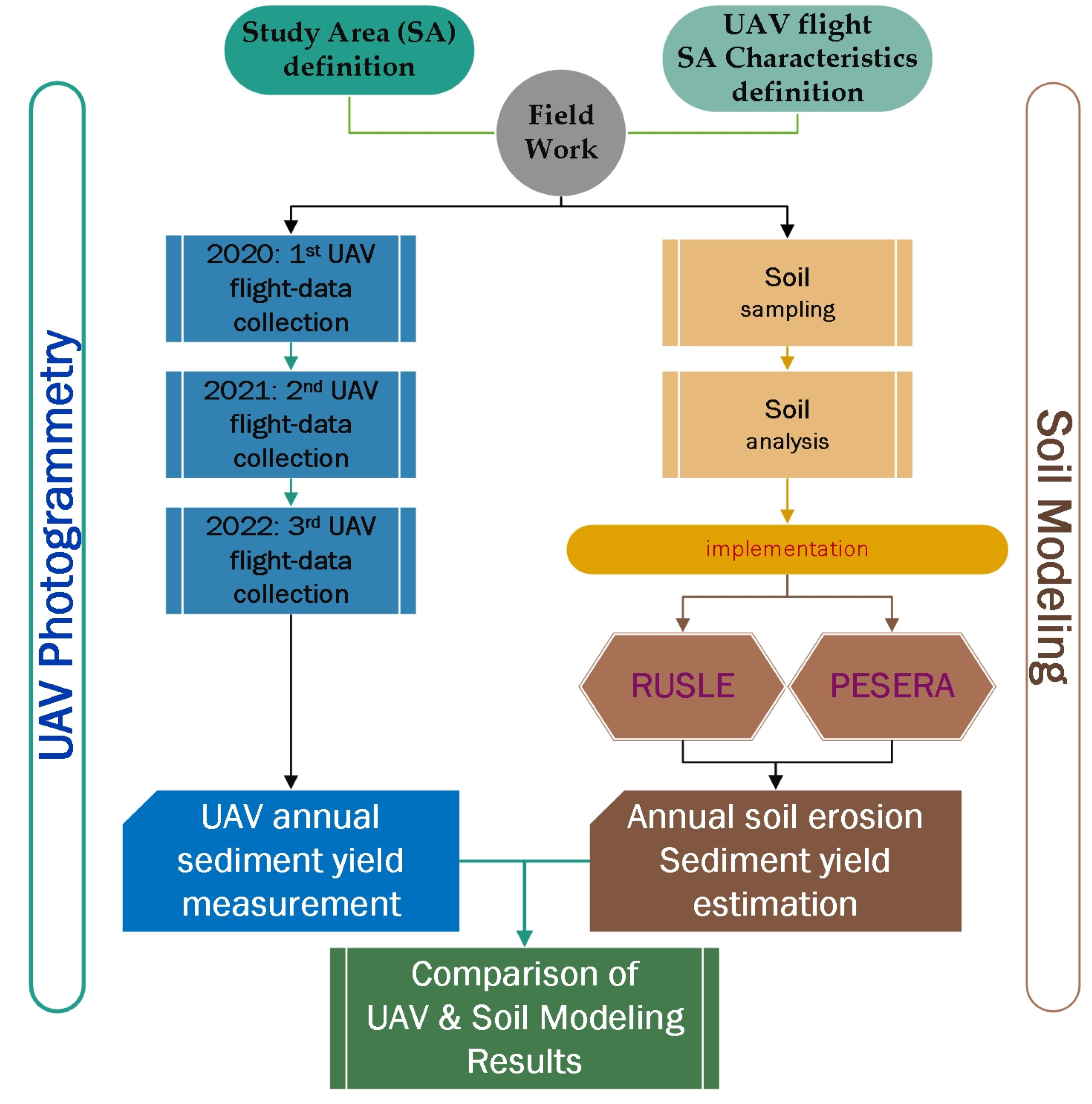
2. Materials and Methods
2.1. Study Area
2.2. Data and Measurements
2.2.1. Earth Observation Data
2.2.2. Geospatial Data
2.3. The Pan European Soil Erosion Risk Assessment (PESERA) Model
2.4. The Revised Universal Soil Loss Equation (RUSLE) Model
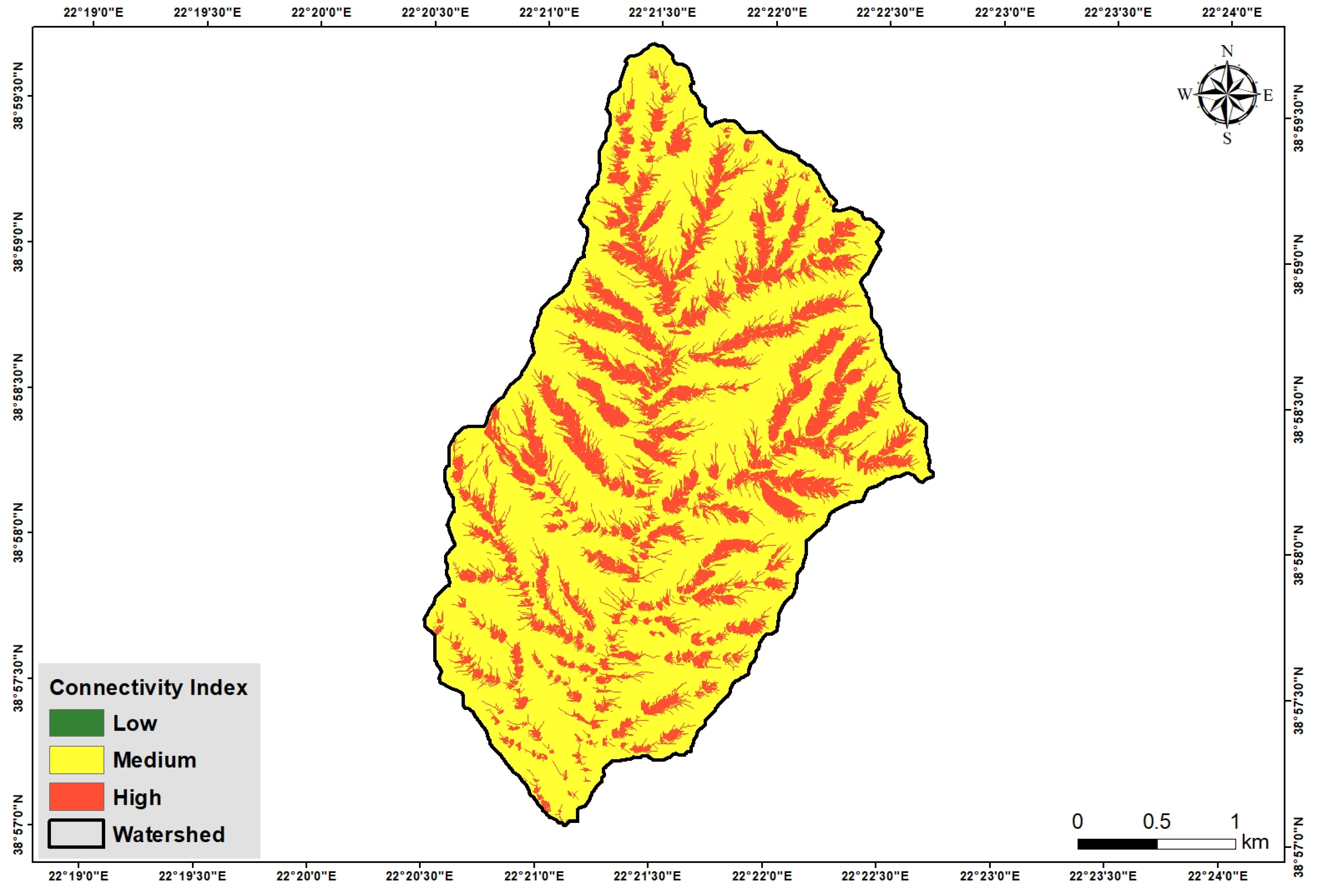
2.5. The Sediment Delivery Ratio (SDR) and Connectivity Index (CI)
3. Results
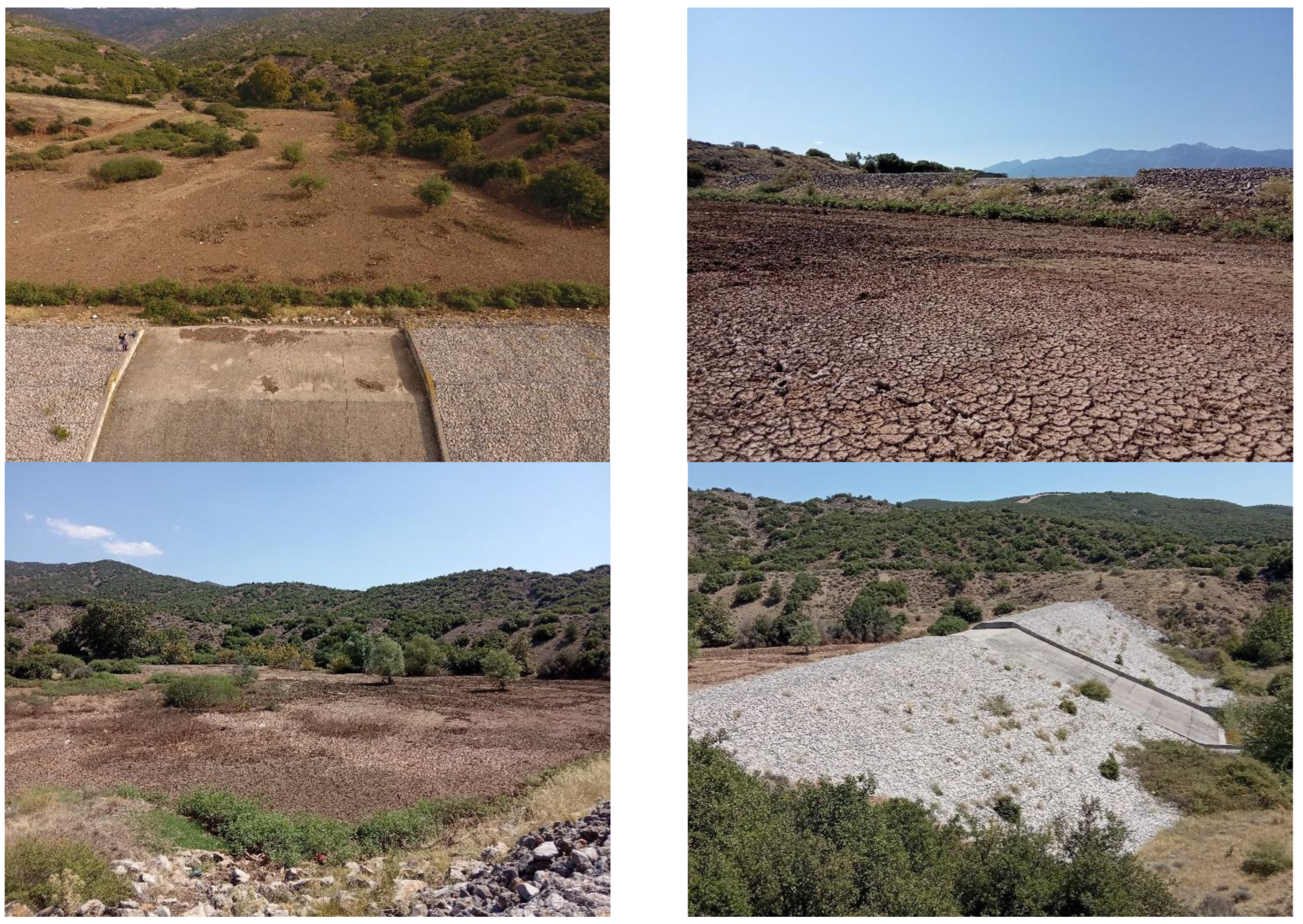
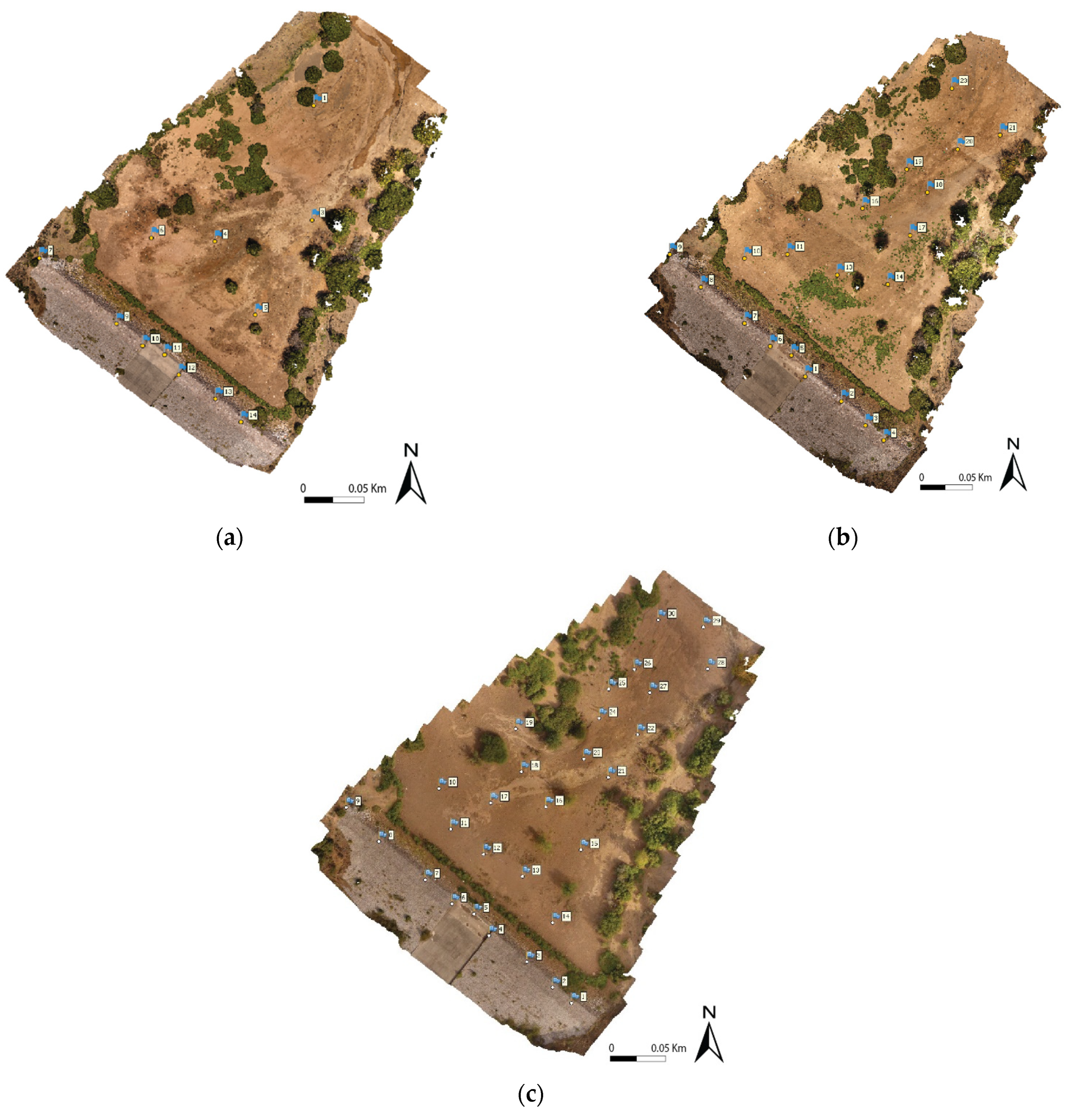
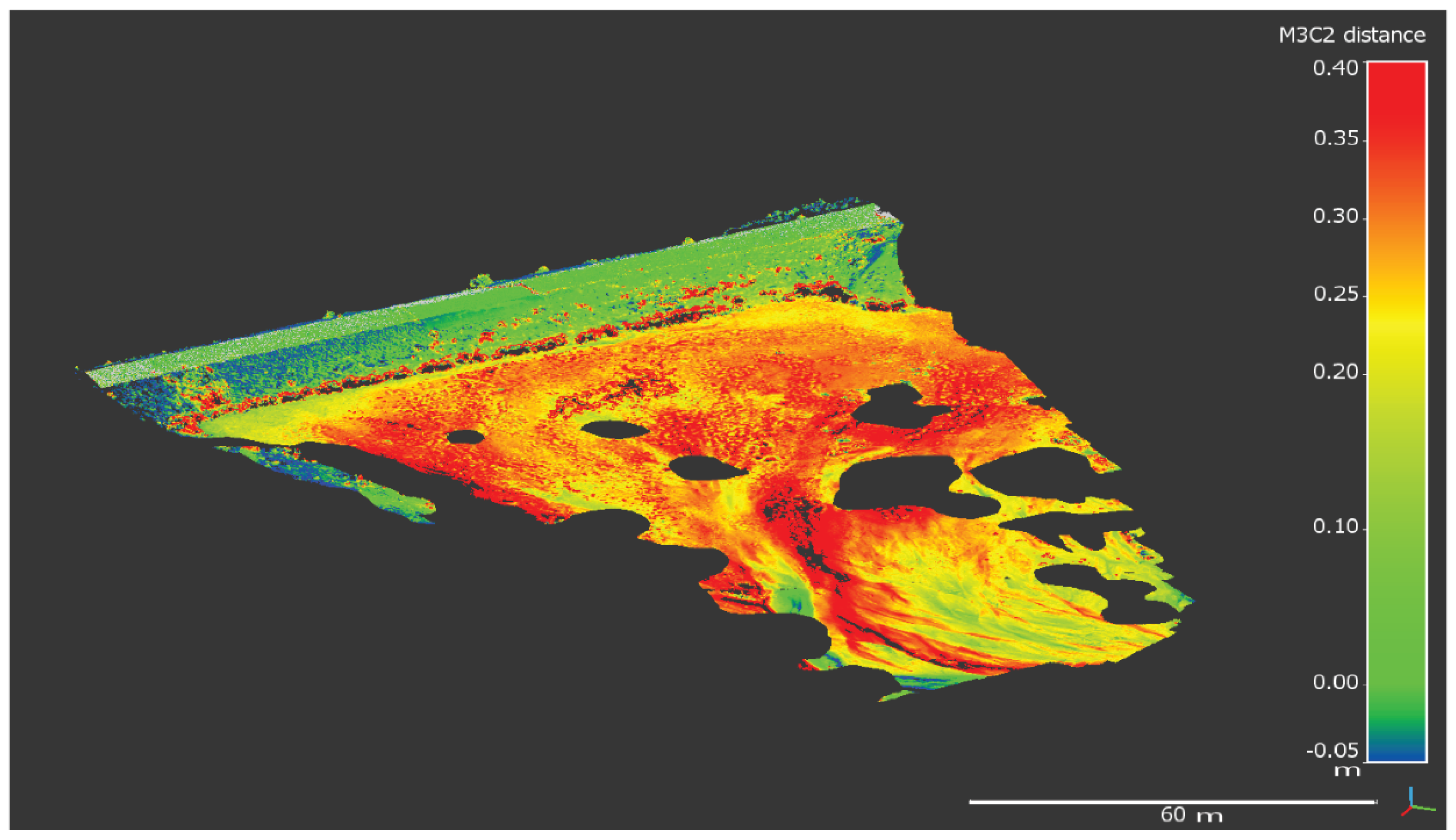
3.1. UAV Photogrammetry and Measurement of the Actual Deposition at the Retention Dam
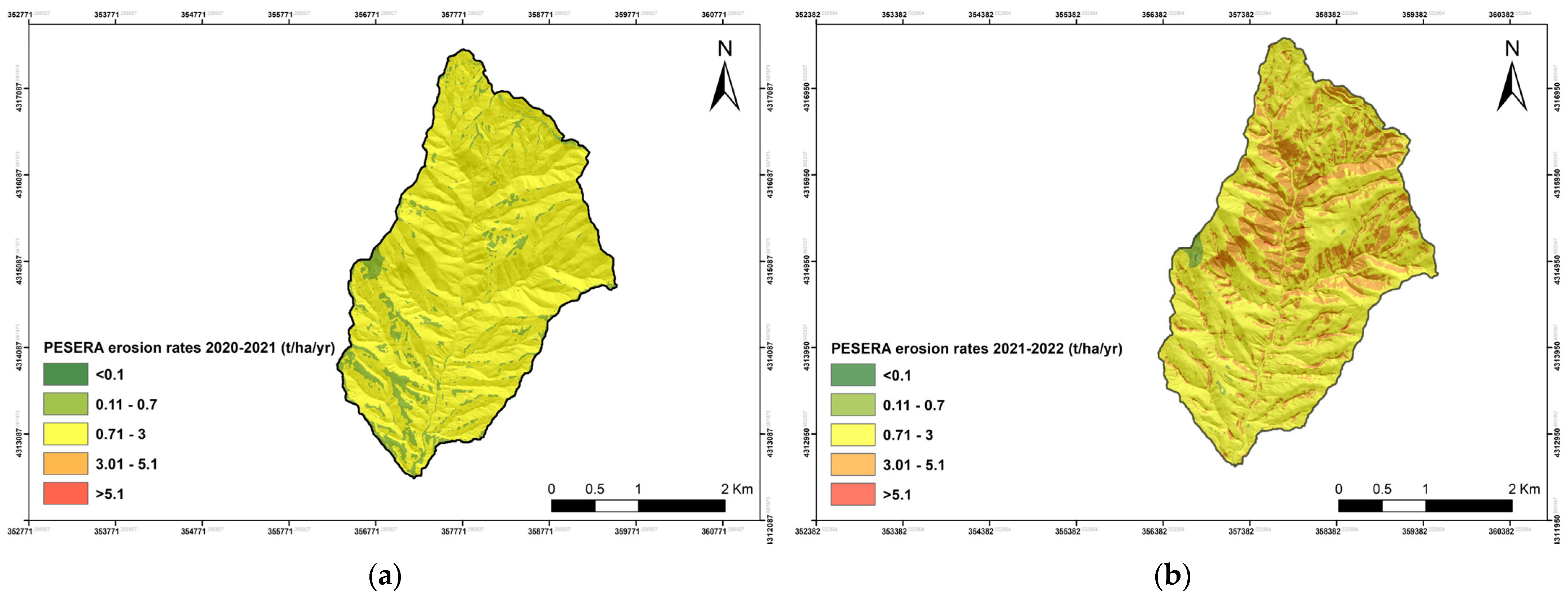
3.2. The PESERA Application
3.3. The RUSLE Application
4. Discussion
5. Conclusions
Author Contributions
Funding
Acknowledgments
Conflicts of Interest
Appendix A. The PESERA Application

| Soil Samples | Texture Code | Texture |
|---|---|---|
| Alluvial deposits | L | 2 |
| Calcareous soils | SL | 1 |
| Volcanic soils | CL | 2 |
| Physical Chemical Erodibility Textural Crusting | 1 Very Low | 2 Low | 3 Medium | 4 High | 5 Very High |
|---|---|---|---|---|---|
| 1 very low | 1 | 1 | 1 | 2 | 3 |
| 2 low | 1 | 2 | 2 | 3 | 5 |
| 3 medium | 2 | 2 | 3 | 4 | 5 |
| 4 high | 2 | 3 | 4 | 4 | 5 |
| 5 very high | 3 | 4 | 5 | 5 | 5 |
| Physical Chemical Erodibility Textural Erodibility | |||||
| 1 very low | 1 | 1 | 1 | 2 | 3 |
| 2 low | 2 | 2 | 2 | 3 | 4 |
| 3 medium | 3 | 3 | 3 | 4 | 5 |
| 4 high | 3 | 4 | 4 | 4 | 5 |
| 5 very high | 4 | 4 | 5 | 5 | 5 |
| Proposed Values | ||
|---|---|---|
| Class | Erodibility | Crusting |
| 1 | 0.1 | 100 |
| 2 | 1 | 20 |
| 3 | 3 | 10 |
| 4 | 6 | 5 |
| 5 | 12 | 2 |
| Parameter | Symbol | Value | Class | Assumption |
|---|---|---|---|---|
| Depth to rock | Dr | 40–80 cm | M | This range of values covers all STUs |
| Depth restriction | Dr_rest Dr_res_10t | 60 cm | M | Given that Dr_rest < 200 cm, Dr_rest = Dr_res_10t |
| Obstacle to roots | Roo | 40–60 cm | 3 | This range of values covers all STUs |
| Topsoil/subsoil Packing Density | Pd_top Pd_sub | 1.4 g/cm3 (Lower value) | L | Laboratory analysis measured for all samples OM < 3% *1 |
| Texture of top/subsoil | Textawctop Textawcsub | Coarse Medium | 1 2 | *1 The texture of the soil samples was within the ranges Clay < 18% & Sand > 65% Clay < 18% & 15% < Sand < 65% and |
| Available water capacity in top- & subsoil | AWC_top2s/2 mm AWC_sub2s/2 mm | 120 mm/m 220 mm/m | Medium Very High | *1 |
| Drainable pores in topsoil | Po_top % | 30 20 | Coarse textured soil Medium-textured soil | |
| Drainable pores in subsoil | Po_sub % | 25 18 | Coarse textured soil Medium-textured soil | |
| Portion of SWAP in top- & subsoil | P1swap_top/sub | 1 | For both the coarse and medium—textured soil | |
| SWSC_eff | 154.5 mm 189 mm | Coarse textured soil Medium-textured soil |
| Soil Texture | Code | zm (mm) |
|---|---|---|
| Coarse | C | 30 |
| Fine | F | 10 |
| Medium | M | 20 |
| Medium fine | MF | 15 |
| Organic soils | O | 10 |
| Very fine | VF | 5 |
| Land Cover Type | Initial Roughness Storage (Rough 0 mm) | % Reduction after 1 Month |
|---|---|---|
| Both (in 1 year) arable | 10 | 50 |
| Cereal-dry farmed | 10 | 50 |
| Natural degraded | 5 | 0 |
| Forest (close canopy) | 5 | 0 |
| Heterogeneous | 5 | 0 |
| Permanent pasture | 5 | 0 |
| Rock, urban, wetlands etc | 0 | 0 |
| Spring sown arable | 10 | 50 |
| Vineyards, tree crops etc | 5 | 0 |
| Autumn sown Med’n arable | 10 | 50 |
| Winter sown arable | 10 | 50 |
| Uncultivated-natural vegetation | 5 | 0 |
| Bare ground | 5 | 0 |
| Model Parameter | Value Range | Input Data Description/Reference |
|---|---|---|
| Land cover type (use) | 240, 320 | CORINE 2018, processed by fieldwork |
| Coverage | 0–100% | Based on FVC and NDVI computed on Google Earth Engine |
| Surface roughness reduction (roughed) | 0.1 | [29] |
| Surface roughness (rough0) | 5 | [29] |
| Root depth | 400, 600 mm | [29] |
| Surface crusting | 20, 40 | [29] |
| Soil erodibility | 2 | [29] |
| Effective Soil Water Storage Capacity (SWSC) | 154.5–189 mm | [13] |
| zm | 20, 30 (mm) | [13] |
| Meteorological data | Value range based on meteorological data (mm) analysis | Processed by the researchers FAO Penman–Monteith equation. (FAO ETo calculator) |
| Standard deviation of elevation | 0–10.01 | Processed by ArcGIS |
Appendix B. The RUSLE Application
| Rain 1 (mm) | Rain 2 (mm) | Energy (MJ ha−1) | EI30 (MJ mm ha−1 h−1) | Erosivity Density * (MJ ha−1 h−1) | |
|---|---|---|---|---|---|
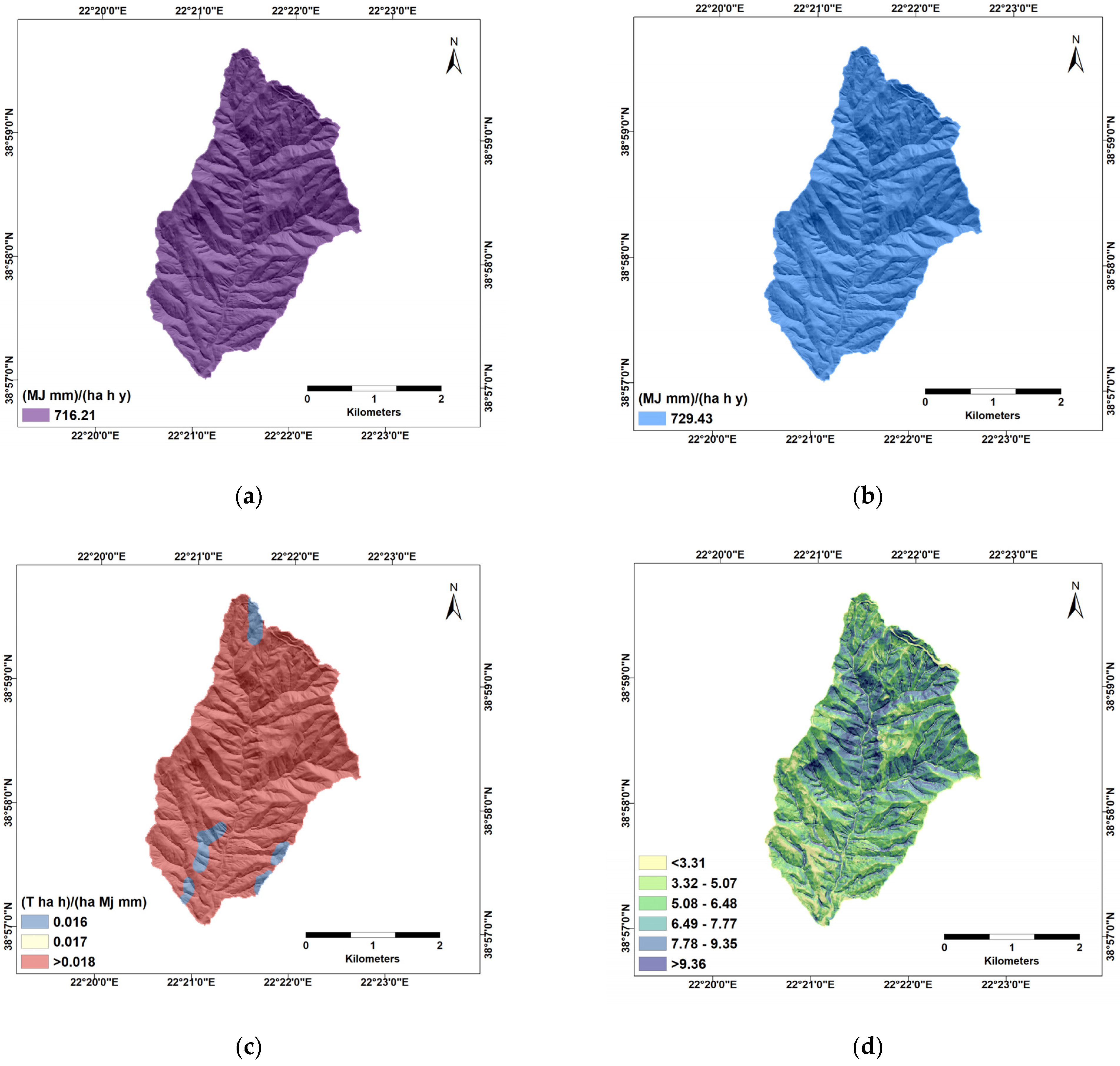
| TOTAL * 2020–2021 | 572.00 | 490.91 | 44.46 | 716.21 | 1.46 |
| TOTAL * 2021–2022 | 793.20 | 599.15 | 74.31 | 729.43 | 1.22 |
| Soil Samples (Texture) | K-Factor |
|---|---|
| Sandy Loam (SL) soil | 0.016 |
| Clay Loam (CL) soil | 0.022 |
| Loam (L) | 0.017 |
References
- Dregne, H.E. Land degradation in the drylands. Arid L. Res. Manag. 2002, 16, 99–132. [Google Scholar] [CrossRef]
- Gao, P.; Pasternack, G.B.; Bali, K.M.; Wallender, W.W. Suspended-sediment transport in an intensively cultivated watershed in southeastern California. Catena 2007, 69, 239–252. [Google Scholar] [CrossRef]
- Carrivick, J.L.; Smith, M.W.; Quincey, D.J. Structure from Motion in the Geosciences; John Wiley & Sons: Hoboken, NJ, USA, 2016; pp. 1–8. [Google Scholar] [CrossRef]
- De Roo, A.P.J.; Hazelhoff, L.; Burrough, P.A. Soil erosion modelling using ‘answers’ and geographical information systems. Earth Surf. Process. Landf. 1989, 14, 517–532. [Google Scholar] [CrossRef]
- Karydas, C.G.; Panagos, P.; Gitas, I.Z. A classification of water erosion models according to their geospatial characteristics. Int. J. Digit. Earth 2014, 7, 229–250. [Google Scholar] [CrossRef]
- Mitra, B.; Scott, H.D.; Dixon, J.C.; McKimmey, J.M. Applications of fuzzy logic to the prediction of soil erosion in a large watershed. Geoderma 1998, 86, 183–209. [Google Scholar] [CrossRef]
- Wischmeier, W.H.; Smith, D.D.; Science and Education Administration, U.S. Department of Agriculture. Predicting Rainfall Erosion Losses: A Guide to Conservation Planning; USDA Publications, Ed.; Science and Education Administration, U.S. Department of Agriculture: Washington, DC, USA, 1978.
- Gavrilovic, Z. The Use of an Empirical Method for Calculating Sediment Production and Transport in Unsuited or Torrential Streams. In Proceedings of the International Conference for Review Regime; Scientific Research Publishing, Ed.; Scientific Research Publishing: Wallingford, UK, 1988; pp. 411–422. [Google Scholar]
- Renard, K.; Foster, G.R.; Weesies, G.; Mccool, D.; Yoder, D. Predicting Soil Erosion by Water: A Guide to Conservation Planning with the Revised Universal Soil Loss Equation (RUSLE); United States Government Printing: Washington, DC, USA, 1997.
- Renard, K.G.; Foster, G.R.; Weesies, G.A.; Porter, J.P. RUSLE: Revised universal soil loss equation. J. Soil Water Conserv. 1991, 46, 30–33. [Google Scholar]
- Laflen, J.M.; Lane, L.J.; Foster, G.R. WEPP: A new generation of erosion prediction technology. J. Soil Water Conserv. 1991, 46, 34–38. [Google Scholar]
- Neitsch, S.L.; Arnold, J.G.; Kiniry, J.R.; Williams, J.R. Soil and Water Assessment Tool Theoretical Documentation; Texas Water Resources Institute, Ed.; Scientific Research Publishing: Wallingford, UK, 2005. [Google Scholar]
- Kirkby, M.J.; Irvine, B.J.; Jones, R.J.A.; Govers, G. The PESERA coarse scale erosion model for Europe. I.—Model rationale and implementation. Eur. J. Soil Sci. 2008, 59, 1293–1306. [Google Scholar] [CrossRef]
- Kirkby, M.J.; Jones, R.J.A.; Irvine, B.; Gobin, A.; Govers, G.; Cerdan, O.; van Rompaey, A.J.J.; le Bissonnais, Y.; Daroussin, J.; King, D.; et al. Pan-European Soil Erosion Risk Assessment: The PESERA Map. 2003. Available online: https://www.researchgate.net/publication/265357850_Pan-European_soil_erosion_risk_assessment_the_PESERA_Map_Version_1_October_2003#fullTextFileContent (accessed on 1 September 2022).
- Karydas, C.G.; Panagos, P. The G2 erosion model: An algorithm for month-time step assessments. Environ. Res. 2018, 161, 256–267. [Google Scholar] [CrossRef]
- Li, P.; Zang, Y.; Ma, D.; Yao, W.; Holden, J.; Irvine, B.; Zhao, G. Soil erosion rates assessed by RUSLE and PESERA for a Chinese Loess Plateau catchment under land-cover changes. Earth Surf. Process. Landf. 2020, 45, 707–722. [Google Scholar] [CrossRef]
- Kaffas, K.; Pisinaras, V.; Al Sayah, M.J.; Santopietro, S.; Righetti, M. A USLE-based model with modified LS-factor combined with sediment delivery module for Alpine basins. Catena 2021, 207, 105655. [Google Scholar] [CrossRef]
- Karamesouti, M.; Petropoulos, G.P.; Papanikolaou, I.D.; Kairis, O.; Kosmas, K. Erosion rate predictions from PESERA and RUSLE at a Mediterranean site before and after a wildfire: Comparison & implications. Geoderma 2016, 261, 44–58. [Google Scholar] [CrossRef]
- Tsara, M.; Kosmas, C.; Kirkby, M.J.; Kosma, D.; Yassoglou, N. An evaluation of the pesera soil erosion model and its application to a case study in Zakynthos, Greece. Soil Use Manag. 2005, 21, 377–385. [Google Scholar] [CrossRef]
- Kinnell, P.I.A. Event soil loss, runoff and the Universal Soil Loss Equation family of models: A review. J. Hydrol. 2010, 385, 384–397. [Google Scholar] [CrossRef]
- De Vente, J.; Poesen, J.; Verstraeten, G.; Govers, G.; Vanmaercke, M.; Van Rompaey, A.; Arabkhedri, M.; Boix-Fayos, C. Predicting soil erosion and sediment yield at regional scales: Where do we stand? Earth-Sci. Rev. 2013, 127, 16–29. [Google Scholar] [CrossRef]
- Esteves, T.C.J.; Kirkby, M.J.; Shakesby, R.A.; Ferreira, A.J.D.; Soares, J.A.A.; Irvine, B.J.; Ferreira, C.S.S.; Coelho, C.O.A.; Bento, C.P.M.; Carreiras, M.A. Mitigating land degradation caused by wildfire: Application of the PESERA model to fire-affected sites in central Portugal. Geoderma 2012, 191, 40–50. [Google Scholar] [CrossRef]
- Vieira, D.C.S.; Malvar, M.C.; Martins, M.A.S.; Serpa, D.; Keizer, J.J. Key factors controlling the post-fire hydrological and erosive response at micro-plot scale in a recently burned Mediterranean forest. Geomorphology 2018, 319, 161–173. [Google Scholar] [CrossRef]
- Fernández, C.; Vega, J.A. Evaluation of RUSLE and PESERA models for predicting soil erosion losses in the first year after wildfire in NW Spain. Geoderma 2016, 273, 64–72. [Google Scholar] [CrossRef]
- Anderson, K.; Ryan, B.; Sonntag, W.; Kavvada, A.; Friedl, L. Earth observation in service of the 2030 Agenda for Sustainable Development. Geo-Spat. Inf. Sci. 2017, 20, 77–96. [Google Scholar] [CrossRef]
- Batista, P.V.G.; Davies, J.; Silva, M.L.N.; Quinton, J.N. On the evaluation of soil erosion models: Are we doing enough? Earth-Sci. Rev. 2019, 197, 102898. [Google Scholar] [CrossRef]
- Alewell, C.; Borrelli, P.; Meusburger, K.; Panagos, P. Using the USLE: Chances, challenges and limitations of soil erosion modelling. Int. Soil Water Conserv. Res. 2019, 7, 203–225. [Google Scholar] [CrossRef]
- Van Rompaey, A.J.; Vieillefont, V.; Jones, R.J.; Montanarella, L.; Verstraeten, G.; Bazzoffi, P.; Dostal, T.; Krasa, J.; de Vente, J.; Poesen, J. Pan-European Soil Erosion Risk Assessment Deliverable 7B: Model Validation at the Catchment Scale. 2003. Available online: https://esdac.jrc.ec.europa.eu/ESDB_Archive/pesera/pesera_cd/pdf/DL7BValidationCatchment.pdf (accessed on 1 September 2022).
- Gobin, A.; Govers, G. Pan-European Soil Erosion Risk Assessment Project. Second Annual Report to the European Commission. EC Contract No. QLK5-CT-1999-01323; EU: Brussels, Belgium, 2002. [Google Scholar]
- Panagos, P.; Borrelli, P.; Meusburger, K.; Alewell, C.; Lugato, E.; Montanarella, L. Estimating the soil erosion cover-management factor at the European scale. Land Use Policy 2015, 48, 38–50. [Google Scholar] [CrossRef]
- Polykretis, C.; Alexakis, D.D.; Grillakis, M.G.; Manoudakis, S. Assessment of Intra-Annual and Inter-Annual Variabilities of Soil Erosion in Crete Island (Greece) by Incorporating the Dynamic “Nature” of R and C-Factors in RUSLE Modeling. Remote Sens. 2020, 12, 2439. [Google Scholar] [CrossRef]
- Sigalos, G.; Loukaidi, V.; Dasaklis, S.; Drakopoulou, P.; Salvati, L.; Ruiz, P.S.; Mavrakis, A. Soil erosion and degradation in a rapidly expanding industrial area of Eastern Mediterranean basin (Thriasio plain, Greece). Nat. Hazards J. Int. Soc. Prev. Mitig. Nat. Hazards 2016, 82, 2187–2200. [Google Scholar] [CrossRef]
- Efthimiou, N.; Lykoudi, E.; Karavitis, C. Comparative analysis of sediment yield estimations using different empirical soil erosion models. Hydrol. Sci. J. 2017, 62, 2674–2694. [Google Scholar] [CrossRef]
- Rozos, D.; Skilodimou, H.D.; Loupasakis, C.; Bathrellos, G.D. Application of the revised universal soil loss equation model on landslide prevention. An example from N. Euboea (Evia) Island, Greece. Environ. Earth Sci. 2013, 70, 3255–3266. [Google Scholar] [CrossRef]
- Walling, D.E. The sediment delivery problem. J. Hydrol. 1983, 65, 209–237. [Google Scholar] [CrossRef]
- Borselli, L.; Cassi, P.; Torri, D. Prolegomena to sediment and flow connectivity in the landscape: A GIS and field numerical assessment. Catena 2008, 75, 268–277. [Google Scholar] [CrossRef]
- Cavalli, M.; Trevisani, S.; Comiti, F.; Marchi, L. Geomorphometric assessment of spatial sediment connectivity in small Alpine catchments. Geomorphology 2013, 188, 31–41. [Google Scholar] [CrossRef]
- Aucelli, P.P.C.; Conforti, M.; Della Seta, M.; Del Monte, M.; D’uva, L.; Rosskopf, C.M.; Vergari, F. Multi-temporal Digital Photogrammetric Analysis for Quantitative Assessment of Soil Erosion Rates in the Landola Catchment of the Upper Orcia Valley (Tuscany, Italy). L. Degrad. Dev. 2016, 27, 1075–1092. [Google Scholar] [CrossRef]
- De Jong, S.M. Derivation of vegetative variables from a landsat tm image for modelling soil erosion. Earth Surf. Process. Landforms 1994, 19, 165–178. [Google Scholar] [CrossRef]
- Meusburger, K.; Bänninger, D.; Alewell, C. Estimating vegetation parameter for soil erosion assessment in an alpine catchment by means of QuickBird imagery. Int. J. Appl. Earth Obs. Geoinf. 2010, 12, 201–207. [Google Scholar] [CrossRef]
- Wang, R.; Zhang, S.; Pu, L.; Yang, J.; Yang, C.; Chen, J.; Guan, C.; Wang, Q.; Chen, D.; Fu, B.; et al. Gully Erosion Mapping and Monitoring at Multiple Scales Based on Multi-Source Remote Sensing Data of the Sancha River Catchment, Northeast China. ISPRS Int. J. Geo-Inf. 2016, 5, 200. [Google Scholar] [CrossRef]
- Efthimiou, N.; Psomiadis, E. The Significance of Land Cover Delineation on Soil Erosion Assessment. Environ. Manag. 2018, 62, 383–402. [Google Scholar] [CrossRef]
- Efthimiou, N.; Psomiadis, E.; Panagos, P. Fire severity and soil erosion susceptibility mapping using multi-temporal Earth Observation data: The case of Mati fatal wildfire in Eastern Attica, Greece. Catena 2020, 187, 104320. [Google Scholar] [CrossRef]
- Alexiou, S.; Deligiannakis, G.; Pallikarakis, A.; Papanikolaou, I.; Psomiadis, E.; Reicherter, K. Comparing High Accuracy t-LiDAR and UAV-SfM Derived Point Clouds for Geomorphological Change Detection. ISPRS Int. J. Geo-Inf. 2021, 10, 367. [Google Scholar] [CrossRef]
- Deligiannakis, G.; Pallikarakis, A.; Papanikolaou, I.; Alexiou, S.; Reicherter, K. Detecting and Monitoring Early Post-Fire Sliding Phenomena Using UAV–SfM Photogrammetry and t-LiDAR-Derived Point Clouds. Fire 2021, 4, 87. [Google Scholar] [CrossRef]
- Kociuba, W.; Janicki, G.; Rodzik, J.; Stępniewski, K. Comparison of volumetric and remote sensing methods (TLS) for assessing the development of a permanent forested loess gully. Nat. Hazards J. Int. Soc. Prev. Mitig. Nat. Hazards 2015, 79, 139–158. [Google Scholar] [CrossRef]
- Longoni, L.; Papini, M.; Brambilla, D.; Barazzetti, L.; Roncoroni, F.; Scaioni, M.; Ivanov, V.I. Monitoring Riverbank Erosion in Mountain Catchments Using Terrestrial Laser Scanning. Remote Sens. 2016, 8, 241. [Google Scholar] [CrossRef]
- D’Oleire-Oltmanns, S.; Marzolff, I.; Peter, K.D.; Ries, J.B. Unmanned Aerial Vehicle (UAV) for Monitoring Soil Erosion in Morocco. Remote Sens. 2012, 4, 3390–3416. [Google Scholar] [CrossRef]
- Eltner, A.; Baumgart, P.; Maas, H.G.; Faust, D. Multi-temporal UAV data for automatic measurement of rill and interrill erosion on loess soil. Earth Surf. Process. Landf. 2015, 40, 741–755. [Google Scholar] [CrossRef]
- Neugirg, F.; Stark, M.; Kaiser, A.; Vlacilova, M.; Della Seta, M.; Vergari, F.; Schmidt, J.; Becht, M.; Haas, F. Erosion processes in calanchi in the Upper Orcia Valley, Southern Tuscany, Italy based on multitemporal high-resolution terrestrial LiDAR and UAV surveys. Geomorphology 2016, 269, 8–22. [Google Scholar] [CrossRef]
- Li, P.; Hao, M.; Hu, J.; Gao, C.; Zhao, G.; Chan, F.K.S.; Gao, J.; Dang, T.; Mu, X. Spatiotemporal Patterns of Hillslope Erosion Investigated Based on Field Scouring Experiments and Terrestrial Laser Scanning. Remote Sens. 2021, 13, 1674. [Google Scholar] [CrossRef]
- Bazzoffi, P. Measurement of rill erosion through a new UAV-GIS methodology. Ital. J. Agron. 2015, 10. [Google Scholar] [CrossRef]
- Borrelli, L.; Conforti, M.; Mercuri, M. LiDAR and UAV System Data to Analyse Recent Morphological Changes of a Small Drainage Basin. ISPRS Int. J. Geo-Inf. 2019, 8, 536. [Google Scholar] [CrossRef]
- Aber, J.; Marzolff, I.; Ries, J.; Aber, S. Small-Format Aerial Photography and UAS Imagery: Principles, Techniques and Geoscience Applications. In Small-Format Aerial Photography and UAS Imagery, 2nd ed.; Academic Press: Cambridge, MA, USA, 2019; pp. 1–382. [Google Scholar] [CrossRef]
- Rieke-Zapp, D.H.; Nearing, M.A. Digital close range photogrammetry for measurement of soil erosion. Photogramm. Rec. 2005, 20, 69–87. [Google Scholar] [CrossRef]
- Marzolff, I.; Poesen, J. The potential of 3D gully monitoring with GIS using high-resolution aerial photography and a digital photogrammetry system. Geomorphology 2009, 111, 48–60. [Google Scholar] [CrossRef]
- Peter, K.D.; d’Oleire-Oltmanns, S.; Ries, J.B.; Marzolff, I.; Ait Hssaine, A. Soil erosion in gully catchments affected by land-levelling measures in the Souss Basin, Morocco, analysed by rainfall simulation and UAV remote sensing data. Catena 2014, 113, 24–40. [Google Scholar] [CrossRef]
- Manfreda, S.; McCabe, M.F.; Miller, P.E.; Lucas, R.; Madrigal, V.P.; Mallinis, G.; Dor, E.B.; Helman, D.; Estes, L.; Ciraolo, G.; et al. On the Use of Unmanned Aerial Systems for Environmental Monitoring. Remote Sens. 2018, 10, 641. [Google Scholar] [CrossRef]
- Yermolaev, O.; Usmanov, B.; Gafurov, A.; Poesen, J.; Vedeneeva, E.; Lisetskii, F.; Nicu, I.C. Assessment of Shoreline Transformation Rates and Landslide Monitoring on the Bank of Kuibyshev Reservoir (Russia) Using Multi-Source Data. Remote Sens. 2021, 13, 4214. [Google Scholar] [CrossRef]
- Meinen, B.U.; Robinson, D.T. Mapping erosion and deposition in an agricultural landscape: Optimization of UAV image acquisition schemes for SfM-MVS. Remote Sens. Environ. 2020, 239, 111666. [Google Scholar] [CrossRef]
- Cândido, B.M.; James, M.; Quinton, J.; de Lima, W.; Silva, M.L.N. Sediment source and volume of soil erosion in a gully system using UAV photogrammetry. Rev. Bras. Ciência Solo 2020, 44, e0200076. [Google Scholar] [CrossRef]
- Cândido, B.M.; Quinton, J.N.; James, M.R.; Silva, M.L.N.; de Carvalho, T.S.; de Lima, W.; Beniaich, A.; Eltner, A. High-resolution monitoring of diffuse (sheet or interrill) erosion using structure-from-motion. Geoderma 2020, 375, 114477. [Google Scholar] [CrossRef]
- Liu, K.; Ding, H.; Tang, G.; Na, J.; Huang, X.; Xue, Z.; Yang, X.; Li, F. Detection of Catchment-Scale Gully-Affected Areas Using Unmanned Aerial Vehicle (UAV) on the Chinese Loess Plateau. ISPRS Int. J. Geo-Inf. 2016, 5, 238. [Google Scholar] [CrossRef]
- Harwin, S.; Lucieer, A. Assessing the Accuracy of Georeferenced Point Clouds Produced via Multi-View Stereopsis from Unmanned Aerial Vehicle (UAV) Imagery. Remote Sens. 2012, 4, 1573–1599. [Google Scholar] [CrossRef]
- Westoby, M.J.; Brasington, J.; Glasser, N.F.; Hambrey, M.J.; Reynolds, J.M. ‘Structure-from-Motion’ photogrammetry: A low-cost, effective tool for geoscience applications. Geomorphology 2012, 179, 300–314. [Google Scholar] [CrossRef]
- Pellicani, R.; Argentiero, I.; Manzari, P.; Spilotro, G.; Marzo, C.; Ermini, R.; Apollonio, C. UAV and Airborne LiDAR Data for Interpreting Kinematic Evolution of Landslide Movements: The Case Study of the Montescaglioso Landslide (Southern Italy). Geosciences 2019, 9, 248. [Google Scholar] [CrossRef]
- Lucieer, A.; Turner, D.; King, D.H.; Robinson, S.A. Using an Unmanned Aerial Vehicle (UAV) to capture micro-topography of Antarctic moss beds. Int. J. Appl. Earth Obs. Geoinf. 2014, 27, 53–62. [Google Scholar] [CrossRef]
- Padró, J.C.; Cardozo, J.; Montero, P.; Ruiz-Carulla, R.; Alcañiz, J.M.; Serra, D.; Carabassa, V. Drone-Based Identification of Erosive Processes in Open-Pit Mining Restored Areas. Land 2022, 11, 212. [Google Scholar] [CrossRef]
- Pineux, N.; Lisein, J.; Swerts, G.; Bielders, C.L.; Lejeune, P.; Colinet, G.; Degré, A. Can DEM time series produced by UAV be used to quantify diffuse erosion in an agricultural watershed? Geomorphology 2017, 280, 122–136. [Google Scholar] [CrossRef]
- Psomiadis, E.; Diakakis, M.; Soulis, K.X. Combining SAR and Optical Earth Observation with Hydraulic Simulation for Flood Mapping and Impact Assessment. Remote Sens. 2020, 12, 3980. [Google Scholar] [CrossRef]
- Psomiadis, E. Long and Short-Term Coastal Changes Assessment Using Earth Observation Data and GIS Analysis: The Case of Sperchios River Delta. ISPRS Int. J. Geo-Inf. 2022, 11, 61. [Google Scholar] [CrossRef]
- Psomiadis, E.; Parcharidis, I.; Stamatis, G.; Foumelis, M. Remotely sensing data and thematic mapping for sustainable developing in Sperchios river basin (Central Greece). Remote Sens. Environ. Monit. GIS Appl. Geol. V 2005, 5983, 408–419. [Google Scholar]
- Psomiadis, E.; Charizopoulos, N.; Soulis, K.X.; Efthimiou, N. Investigating the Correlation of Tectonic and Morphometric Characteristics with the Hydrological Response in a Greek River Catchment Using Earth Observation and Geospatial Analysis Techniques. Geosciences 2020, 10, 377. [Google Scholar] [CrossRef]
- Marinos, G.; Papastamatiou, J.; Maratos, G.; Melidonis, N.; Andronopoulos, B.; Tataris, A.; Betoulis, D.K.G.; Maragoudakis, N.; Lalechos, N. Geological Map of Greece, Lamia Sheet, Scale 1:50.000 1967.
- Bouyoucos, G.J. Hydrometer Method Improved for Making Particle Size Analyses of Soils1. Agron. J. 1962, 54, 464–465. [Google Scholar] [CrossRef]
- Walkley, A.J.; Black, I.A. Estimation of soil organic carbon by the chromic acid titration method. Soil Sci. 1934, 37, 29–38. [Google Scholar] [CrossRef]
- Puliti, S.; Ørka, H.O.; Gobakken, T.; Næsset, E. Inventory of Small Forest Areas Using an Unmanned Aerial System. Remote Sens. 2015, 7, 9632–9654. [Google Scholar] [CrossRef]
- Fraser, B.T.; Congalton, R.G. Issues in Unmanned Aerial Systems (UAS) Data Collection of Complex Forest Environments. Remote Sens. 2018, 10, 908. [Google Scholar] [CrossRef]
- de Lima, R.S.; Lang, M.; Burnside, N.G.; Peciña, M.V.; Arumäe, T.; Laarmann, D.; Ward, R.D.; Vain, A.; Sepp, K. An Evaluation of the Effects of UAS Flight Parameters on Digital Aerial Photogrammetry Processing and Dense-Cloud Production Quality in a Scots Pine Forest. Remote Sens. 2021, 13, 1121. [Google Scholar] [CrossRef]
- Tomaštík, J.; Mokroš, M.; Surový, P.; Grznárová, A.; Merganič, J. UAV RTK/PPK Method—An Optimal Solution for Mapping Inaccessible Forested Areas? Remote Sens. 2019, 11, 721. [Google Scholar] [CrossRef]
- Sona, G.; Pinto, L.; Pagliari, D.; Passoni, D.; Gini, R. Experimental analysis of different software packages for orientation and digital surface modelling from UAV images. Earth Sci. Inform. 2014, 7, 97–107. [Google Scholar] [CrossRef]
- Kaiser, A.; Neugirg, F.; Rock, G.; Müller, C.; Haas, F.; Ries, J.; Schmidt, J. Small-Scale Surface Reconstruction and Volume Calculation of Soil Erosion in Complex Moroccan Gully Morphology Using Structure from Motion. Remote Sens. 2014, 6, 7050–7080. [Google Scholar] [CrossRef]
- Monserrat, O.; Crosetto, M. Deformation measurement using terrestrial laser scanning data and least squares 3D surface matching. ISPRS J. Photogramm. Remote Sens. 2008, 63, 142–154. [Google Scholar] [CrossRef]
- Lague, D.; Brodu, N.; Leroux, J. Accurate 3D comparison of complex topography with terrestrial laser scanner: Application to the Rangitikei canyon (N-Z). ISPRS J. Photogramm. Remote Sens. 2013, 82, 10–26. [Google Scholar] [CrossRef]
- Rouse, J.W.J.; Haas, R.H.; Schell, J.A.; Deering, D.W.; Haas, R.H.; Schell, J.A.; Deering, D.W. Monitoring Vegetation Systems in the Great Plains with ERTS; NASA Special Publications: Washington, DC, USA, 1974. [Google Scholar]
- Niu, B.; Hong, S.; Yuan, J.; Peng, S.; Wang, Z.; Zhang, X. Global trends in sediment-related research in earth science during 1992–2011: A bibliometric analysis. Scientometrics 2014, 98, 511–529. [Google Scholar] [CrossRef]
- Yang, X.; Yang, X. Deriving RUSLE cover factor from time-series fractional vegetation cover for hillslope erosion modelling in New South Wales. Soil Res. 2014, 52, 253–261. [Google Scholar] [CrossRef]
- Sun, W.; Shao, Q.; Liu, J.; Zhai, J. Assessing the effects of land use and topography on soil erosion on the Loess Plateau in China. Catena 2014, 121, 151–163. [Google Scholar] [CrossRef]
- Zhongming, W.; Lees, B.G.; Feng, J.; Wanning, L.; Haijing, S. Stratified vegetation cover index: A new way to assess vegetation impact on soil erosion. Catena 2010, 83, 87–93. [Google Scholar] [CrossRef]
- Mikulicic, N.; Mihajlovic, Z. Procedural generation of mediterranean environments. In Proceedings of the 2016 39th International Convention on Information and Communication Technology, Electronics and Microelectronics (MIPRO), Opatija, Croatia, 30 May 2016–3 June 2016; pp. 261–266. [Google Scholar] [CrossRef]
- Efthimiou, N.; Psomiadis, E.; Papanikolaou, I.; Soulis, K.X.; Borrelli, P.; Panagos, P. A new high resolution object-oriented approach to define the spatiotemporal dynamics of the cover-management factor in soil erosion modelling. Catena 2022, 213, 106149. [Google Scholar] [CrossRef]
- Boettinger, J.L.; Ramsey, R.D.; Bodily, J.M.; Cole, N.J.; Kienast-Brown, S.; Nield, S.J.; Saunders, A.M.; Stum, A.K. Landsat spectral data for digital soil mapping. In Digital Soil Mapping with Limited Data; Springer: Dordrecht, The Netherlands, 2008; pp. 193–202. [Google Scholar] [CrossRef]
- Zeng, X.; Dickinson, R.E.; Walker, A.; Shaikh, M.; Defries, R.S.; Qi, J.; Zeng, X.; Dickinson, R.E.; Walker, A.; Shaikh, M.; et al. Derivation and Evaluation of Global 1-km Fractional Vegetation Cover Data for Land Modeling. JApMe 2000, 39, 826–839. [Google Scholar] [CrossRef]
- Gutman, G.; Ignatov, A. The derivation of the green vegetation fraction from NOAA/AVHRR data for use in numerical weather prediction models. Int. J. Remote Sens. 2010, 19, 1533–1543. [Google Scholar] [CrossRef]
- Helman, D.; Lensky, I.M.; Tessler, N.; Osem, Y.; Helmer, E.H.; Atzberger, C.; Thenkabail, P.S. A Phenology-Based Method for Monitoring Woody and Herbaceous Vegetation in Mediterranean Forests from NDVI Time Series. Remote Sens. 2015, 7, 12314–12335. [Google Scholar] [CrossRef]
- Sagris, V.; Dittmann, C.; Devos, W. Towards the core conceptual LPIS model. In Proceedings of the JRC LPIS Workshop—LPIS Database Quality Assessment and Updating; JRC: Ispra, Italy, 2007. [Google Scholar]
- Cilek, A.; Berberoglu, S.; Kirkby, M.; Irvine, B.; Donmez, C.; Erdogan, M.A. Erosion modelling in a Mediterranean Subcatchment under climate change scenarios using Pan-European Soil Erosion Risk Assessment (PESERA). Int. Arch. Photogramm. Remote Sens. Spat. Inf. Sci. -ISPRS Arch. 2015, 40, 359–365. [Google Scholar] [CrossRef]
- Djuma, H.; Bruggeman, A.; Camera, C.; Zoumides, C. Combining Qualitative and Quantitative Methods for Soil Erosion Assessments: An Application in a Sloping Mediterranean Watershed, Cyprus. Land Degrad. Dev. 2017, 28, 243–254. [Google Scholar] [CrossRef]
- Kouli, M.; Soupios, P.; Vallianatos, F. Soil erosion prediction using the Revised Universal Soil Loss Equation (RUSLE) in a GIS framework, Chania, Northwestern Crete, Greece. Environ. Geol. 2009, 57, 483–497. [Google Scholar] [CrossRef]
- Brini, I.; Alexakis, D.D.; Kalaitzidis, C. Linking Soil Erosion Modeling to Landscape Patterns and Geomorphometry: An Application in Crete, Greece. Appl. Sci. 2021, 11, 5684. [Google Scholar] [CrossRef]
- Hooke, J.; Souza, J.; Marchamalo, M. Evaluation of connectivity indices applied to a Mediterranean agricultural catchment. Catena 2021, 207, 105713. [Google Scholar] [CrossRef]
- Surian, N.; Righini, M.; Lucía, A.; Nardi, L.; Amponsah, W.; Benvenuti, M.; Borga, M.; Cavalli, M.; Comiti, F.; Marchi, L.; et al. Channel response to extreme floods: Insights on controlling factors from six mountain rivers in northern Apennines, Italy. Geomorphology 2016, 272, 78–91. [Google Scholar] [CrossRef]
- Vigiak, O.; Newham, L.; Whitford, J.; Melland, A.; Borselli, L. Comparison of landscape approaches to define spatial patterns of hillslope-scale sediment delivery ratio. In Proceedings of the 18th World IMACS Congress and International Congress on Modelling and Simulation (MODSIM09), Cairns, Australia, 13–17 July 2009; pp. 3123–3129. [Google Scholar]
- Sedighi, F.; Khaledi Darvishan, A.; Zare, M.R.; Sedighi, F.; Khaledi Darvishan, A.; Zare, M.R. Effect of watershed geomorphological characteristics on sediment redistribution. Geomo 2021, 375, 107559. [Google Scholar] [CrossRef]
- Vanoni, V.A. Sedimentation Engineering. Am. Soc. Civ. Eng. 2006, 1–418. [Google Scholar] [CrossRef]
- Maner, S.B. Factors Influencing Sediment Delivery Ratios in the Blackland Prairie Land Resource Area; U.S. Department of Agriculture: Washington, DC, USA, 1962.
- Renfro, W.G. Use of erosion equation and sediment delivery ratios for predicting sediment yield. In Present and Prospective Tecnology for Predicting Sediment Yields and Sources; U.S. Department of Agriculture: Washington, DC, USA, 1975; Volume ARS-S-40, pp. 33–45. [Google Scholar]
- USDA. Sediment Sources, Yields, and Delivery Ratios. In National Engineering Handbook; US Soil Conservation Service: Washington, DC, USA, 1975. [Google Scholar]
- Lagouvardos, K.; Karagiannidis, A.; Dafis, S.; Kalimeris, A.; Kotroni, V. Ianos—A Hurricane in the Mediterranean. Bull. Am. Meteorol. Soc. 2022, 103, E1621–E1636. [Google Scholar] [CrossRef]
- Morgan, R.P.C. A simple approach to soil loss prediction: A revised Morgan-Morgan-Finney model. Catena 2001, 44, 305–322. [Google Scholar] [CrossRef]
- Morgan, R.P.C.; Duzant, J.H. Modified MMF (Morgan–Morgan–Finney) model for evaluating effects of crops and vegetation cover on soil erosion. Earth Surf. Process. Landf. 2008, 33, 90–106. [Google Scholar] [CrossRef]
- Collins, A.L.; Walling, D.E.; Sichingabula, H.M.; Leeks, G.J.L. Using 137Cs measurements to quantify soil erosion and redistribution rates for areas under different land use in the Upper Kaleya River basin, southern Zambia. Geoderma 2001, 104, 299–323. [Google Scholar] [CrossRef]
- Eltner, A.; Schneider, D. Analysis of Different Methods for 3D Reconstruction of Natural Surfaces from Parallel-Axes UAV Images. Photogramm. Rec. 2015, 30, 279–299. [Google Scholar] [CrossRef]
- Thamm, H.P.; Judex, M. The ‘Low-Cost Drone’—An Interesting Tool for Process Monitoring in a High Spatial and Temporal Resolution. In Proceedings of the ISPRS Commission VII Mid-Term Symposium ‘Remote Sensing from Pixels to Processes’; ISPRS Archives: Enschede, The Netherlands, 2006; pp. 140–144. [Google Scholar]
- Wang, R.; Sun, H.; Yang, J.; Zhang, S.; Fu, H.; Wang, N.; Liu, Q.; Wang, R.; Sun, H.; Yang, J.; et al. Quantitative Evaluation of Gully Erosion Using Multitemporal UAV Data in the Southern Black Soil Region of Northeast China: A Case Study. Remote Sens. 2022, 14, 1479. [Google Scholar] [CrossRef]
- Turner, D.; Lucieer, A.; Watson, C. An Automated Technique for Generating Georectified Mosaics from Ultra-High Resolution Unmanned Aerial Vehicle (UAV) Imagery, Based on Structure from Motion (SfM) Point Clouds. Remote Sens. 2012, 4, 1392–1410. [Google Scholar] [CrossRef]
- Andaru, R.; Cahyono, B.K.; Riyadi, G.; Istarno; Djurdjani; Ramadhan, G.R.; Tuntas, S. The combination of terrestrial LiDAR and UAV photogrammetry for interactive architectural heritage visualization using unity 3D game engine. Int. Arch. Photogramm. Remote Sens. Spat. Inf. Sci. 2019, XLII-2-W17, 39–44. [Google Scholar] [CrossRef]
- Stumpf, A.; Malet, J.P.; Kerle, N.; Niethammer, U.; Rothmund, S. Image-based mapping of surface fissures for the investigation of landslide dynamics. Geomorphology 2013, 186, 12–27. [Google Scholar] [CrossRef]
- Cao, L.; Liu, H.; Fu, X.; Zhang, Z.; Shen, X.; Ruan, H. Comparison of UAV LiDAR and Digital Aerial Photogrammetry Point Clouds for Estimating Forest Structural Attributes in Subtropical Planted Forests. Forests 2019, 10, 145. [Google Scholar] [CrossRef]
- Kowalski, A.; Wajs, J.; Kasza, D. Monitoring of anthropogenic landslide activity with combined UAV and lidar-derived dems —A case study of the czerwony wąwóz landslide (SW Poland, western sudetes). Acta Geodyn. Geomater. 2018, 15, 117–129. [Google Scholar] [CrossRef]
- Ulvi, A. The effect of the distribution and numbers of ground control points on the precision of producing orthophoto maps with an unmanned aerial vehicle. J. Asian Archit. Build. Eng. 2021, 20, 806–817. [Google Scholar] [CrossRef]
- Yang, J.; Li, X.; Luo, L.; Zhao, L.; Wei, J.; Ma, T. New Supplementary Photography Methods after the Anomalous of Ground Control Points in UAV Structure-from-Motion Photogrammetry. Drones 2022, 6, 105. [Google Scholar] [CrossRef]
- Waltner, I.; Saeidi, S.; Grósz, J.; Centeri, C.; Laborczi, A.; Pásztor, L. Spatial Assessment of the Effects of Land Cover Change on Soil Erosion in Hungary from 1990 to 2018. ISPRS Int. J. Geo-Inf. 2020, 9, 667. [Google Scholar] [CrossRef]
- Yassoglou, N.J.; Kosmas, C. Desertification in the Mediterranean Europe. A case in Greece. Communities 2000, 27–33. [Google Scholar]
- Kosmas, C.; Danalatos, N.; Cammeraat, L.H.; Chabart, M.; Diamantopoulos, J.; Farand, R.; Gutierrez, L.; Jacob, A.; Marques, H.; Martinez-Fernandez, J.; et al. The effect of land use on runoff and soil erosion rates under Mediterranean conditions. Catena 1997, 29, 45–59. [Google Scholar] [CrossRef]
- Stefanidis, S.; Alexandridis, V.; Ghosal, K. Assessment of Water-Induced Soil Erosion as a Threat to Natura 2000 Protected Areas in Crete Island, Greece. Sustainability 2022, 14, 2738. [Google Scholar] [CrossRef]
- de Vente, J.; Poesen, J.; Verstraeten, G.; Van Rompaey, A.; Govers, G. Spatially distributed modelling of soil erosion and sediment yield at regional scales in Spain. Glob. Planet. Change 2008, 60, 393–415. [Google Scholar] [CrossRef]
- Cerdan, O.; Govers, G.; Le Bissonnais, Y.; Van Oost, K.; Poesen, J.; Saby, N.; Gobin, A.; Vacca, A.; Quinton, J.; Auerswald, K.; et al. Rates and spatial variations of soil erosion in Europe: A study based on erosion plot data. Geomorphology 2010, 122, 167–177. [Google Scholar] [CrossRef]
- Borrelli, P.; Märker, M.; Panagos, P.; Schütt, B. Modeling soil erosion and river sediment yield for an intermountain drainage basin of the Central Apennines, Italy. Catena 2014, 114, 45–58. [Google Scholar] [CrossRef]
- Baggaley, N.; Potts, J. Sensitivity of the PESERA soil erosion model to terrain and soil inputs. Geoderma Reg. 2017, 11, 104–112. [Google Scholar] [CrossRef]
- Panagos, P.; Meusburger, K.; Ballabio, C.; Borrelli, P.; Alewell, C. Soil erodibility in Europe: A high-resolution dataset based on LUCAS. Sci. Total Environ. 2014, 479–480, 189–200. [Google Scholar] [CrossRef]
- Boomer, K.B.; Weller, D.E.; Jordan, T.E. Empirical Models Based on the Universal Soil Loss Equation Fail to Predict Sediment Discharges from Chesapeake Bay Catchments. J. Environ. Qual. 2008, 37, 79–89. [Google Scholar] [CrossRef]
- Diodato, N.; Grauso, S. An improved correlation model for sediment delivery ratio assessment. Environ. Earth Sci. 2009, 59, 223–231. [Google Scholar] [CrossRef]
- Lenhart, T.; Van Rompaey, A.; Steegen, A.; Fohrer, N.; Frede, H.G.; Govers, G. Considering spatial distribution and deposition of sediment in lumped and semi-distributed models. Hydrol. Process. 2005, 19, 785–794. [Google Scholar] [CrossRef]
- Cerdà, A.; Bagarello, V.; Ferro, V.; Estaban, M.; Borja, L.; Francisco, J.; Murillo, M.; González Camarena, R. The scale effect on soil erosion. A plot approach to understand connectivity on slopes under cultivation at variable plot sizes and under Mediterranean climatic conditions. Geophys. Res. Abstr. 2017, 19, 2017–18042. [Google Scholar] [CrossRef]
- Williams, J.R. Sediment delivery ratios determiner with sediment and runoff models. Int. Assoc. Hydrol. Sci. Publ. 1977, 122, 168–179. [Google Scholar]
- Sloff, C.J. Reservoir sedimentation; a literature survey. In Communications on Hydraulic and Geotechnical Engineering, No. 1991-02; TU Delft: Delft, The Netherlands, 1991. [Google Scholar]
- Schleiss, A.J.; Franca, M.J.; Juez, C.; De Cesare, G. Reservoir sedimentation. J. Hydraul. Res. 2016, 54, 595–614. [Google Scholar] [CrossRef]
- Lagouvardos, K.; Kotroni, V.; Bezes, A.; Koletsis, I.; Kopania, T.; Lykoudis, S.; Mazarakis, N.; Papagiannaki, K.; Vougioukas, S. The automatic weather stations NOANN network of the National Observatory of Athens: Operation and database. Geosci. Data J. 2017, 4, 4–16. [Google Scholar] [CrossRef]
- Le Bissonnais, Y.; Daroussin, J.J.; Jamagne, M.; Lambert, J.J.; Le Bas, C.; King, D.D.; Cerdan, O.; Léonard, J.J.; Bresson, L.M.; Jones, R.J.A. Pan-European soil crustingand erodibility assessment from the European soil geographicaldatabase using pedotransfer rules. Adv. Environ. Monit. Model. 2005, 2, 1–15. [Google Scholar]
- Richards, L.A. The Usefulness of Capillary Potential to Soil-Moisture and Plant Investigators. J. Agric. Res. 1928, 37, 719–742. [Google Scholar]
- da Silva, A.P.; Kay, B.D.; Perfect, E.; da Silva, A.; Kay, B. Characterization of the Least Limiting Water Range of Soils. Soil Sci. Soc. Am. J. 1994, 58, 1775–1781. [Google Scholar] [CrossRef]
- Rabot, E.; Wiesmeier, M.; Schlüter, S.; Vogel, H.J. Soil structure as an indicator of soil functions: A review. Geoderma 2018, 314, 122–137. [Google Scholar] [CrossRef]
- Beven, K.; Kirkby, M.; Freer, J.E.; Lamb, R. A history of TOPMODEL. Hydrol. Earth Syst. Sci. 2021, 25, 527–549. [Google Scholar] [CrossRef]
- Beven, K.J.; Kirkby, M.J. A physically based, variable contributing area model of basin hydrology/Un modèle à base physique de zone d’appel variable de l’hydrologie du bassin versant. Hydrol. Sci. J. 2009, 24, 43–69. [Google Scholar] [CrossRef]
- Zotarelli, L.; Dukes, M.D.; Romero, C.C.; Migliaccio, K.W.; Morgan, K.T. Step by Step Calculation of the Penman-Monteith Evapotranspiration (FAO-56 Method); Institute of Food and Agricultural Sciences, University of Florida: Gainesville, FL, USA, 2013. [Google Scholar]
- Wischmeier, W.H. A Rainfall Erosion Index for a Universal Soil-Loss Equation. Soil Sci. Soc. Am. J. 1959, 23, 246–249. [Google Scholar] [CrossRef]
- RIST—Rainfall Intensity Summarization Tool: USDA ARS. Available online: https://www.ars.usda.gov/southeast-area/oxford-ms/national-sedimentation-laboratory/watershed-physical-processes-research/research/rist/rist-rainfall-intensity-summarization-tool/ (accessed on 28 December 2022).
- Lykoudi, E.; Zarris, D. Identification of regions with high risk of soil erosion in the island of Cephalonia using the Universal Soil Loss Equation. In Proceedings of the Sixth National Conference of the Geographical Society of Greece, Thessaloniki, Greece, 3–6 October 2002; pp. 412–419. [Google Scholar]
- Desmet, P.J.J.; Govers, G. A GIS Procedure for Automatically Calculating the USLE LS Factor on Topographically Complex Landscape Units. J. Soil Water Conserv. 1996, 51, 427–433. [Google Scholar]
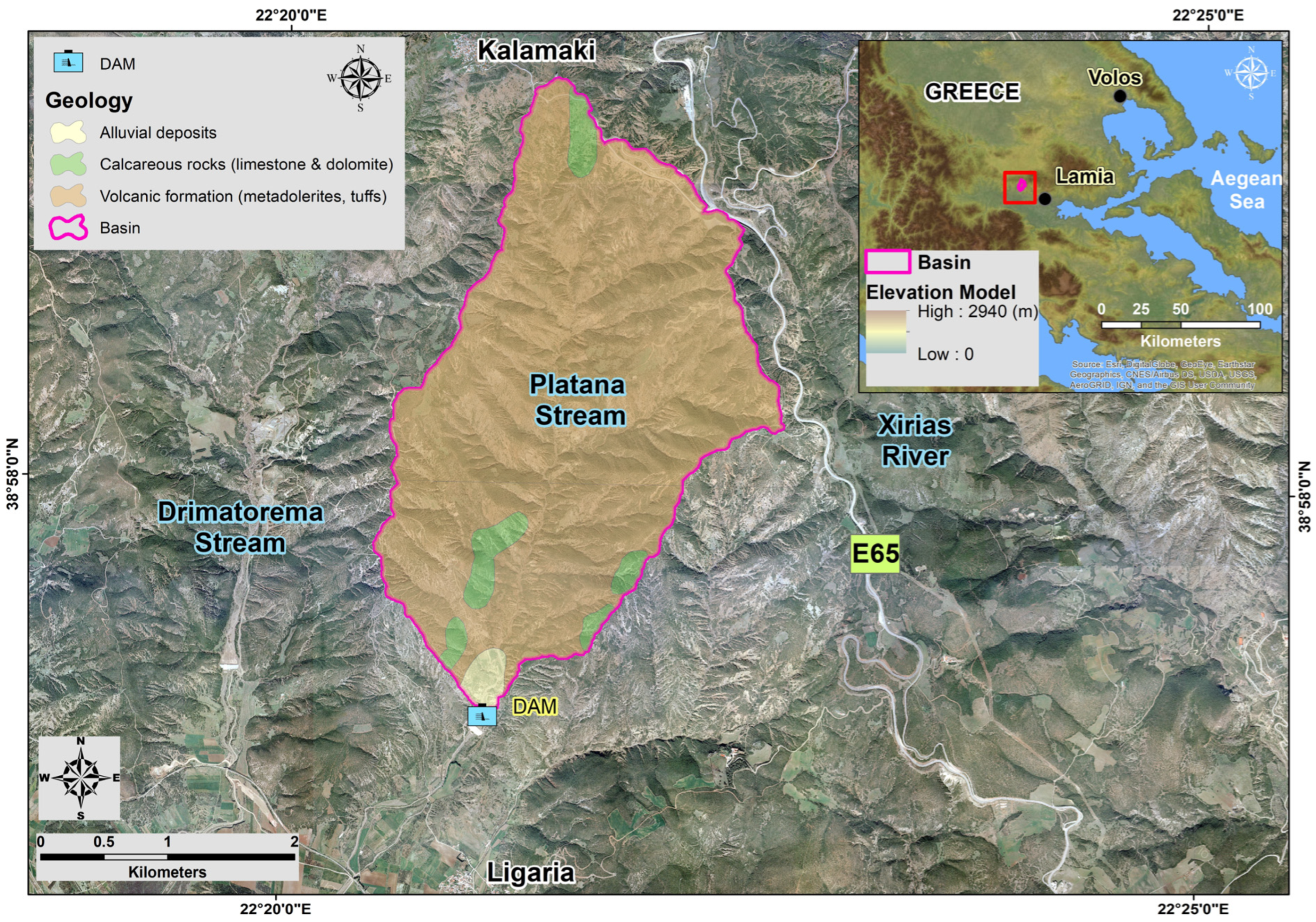


| Latitude (N) | 350,206 |
| Longitude (E) | 4,313,396 |
| Type | Earth Dam |
| Dam crest height (m) | 205.50 |
| Dam crest length (m) | 208.00 |
| Spillway crest length (m) | 20.00 |
| Maximum retention volume (m3) | 140,000 |
| Resolution mm/pix | |||
|---|---|---|---|
| Product | 28 August 2020 | 16 September 2021 | 13 October 2022 |
| Tiled model | 10 | 7 | 10 |
| DEM | 20 | 14.8 | 17 |
| Orthomosaic | 10 | 7.4 | 8.6 |
| Period | Sep | Oct | Nov | Dec | Jan | Feb | Mar | Apr | May | Jun | Jul | Aug | Sep | Total |
|---|---|---|---|---|---|---|---|---|---|---|---|---|---|---|
| 09.2020–08.2021 | 148.2 | 33.6 | 9.8 | 84.0 | 91.4 | 46.6 | 58.6 | 49.2 | 2.0 | 30.2 | 7.6 | 10.8 | 572.0 | |
| 10.2021–09.2022 | 115.8 | 133.8 | 155.8 | 76.6 | 53.2 | 60.8 | 26.4 | 49.2 | 71.2 | 28.8 | 19.6 | 2.0 | 793.2 |
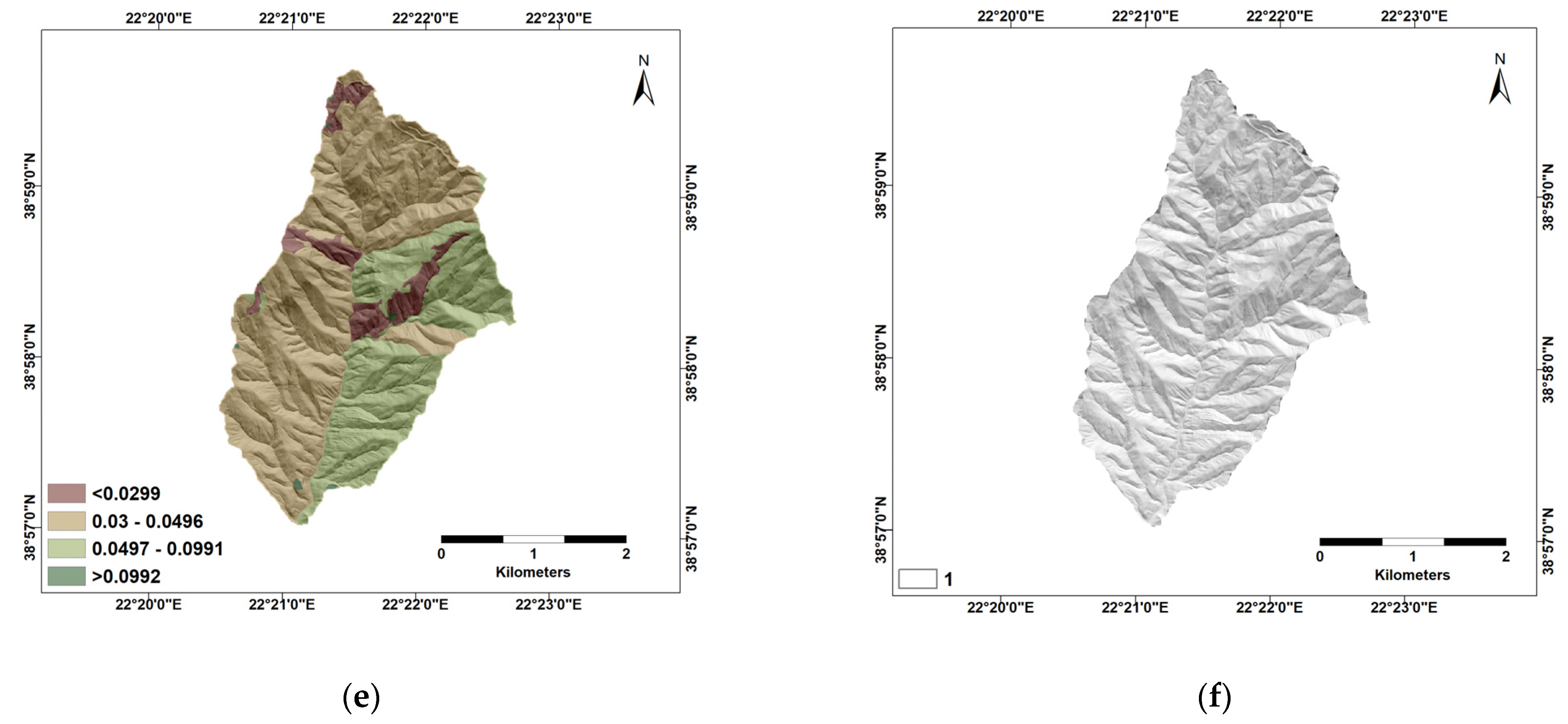
| Level 1 | LULC * Level 3 a | Status | Area (km2) | C-Factor |
|---|---|---|---|---|
| Agricultural areas | 211 | Arable | 0.019 | 0.3 |
| 223 | Non-arable | 0.009 | 0.1 | |
| 231 | Non-arable | 0.669 | 0.02 | |
| 243 | Non-arable | 0.027 | 0.07 | |
| Forest and semi-natural areas | 321 | Non-arable | 2.734 | 0.05 |
| 323 | Non-arable | 5.231 | 0.03 |
Disclaimer/Publisher’s Note: The statements, opinions and data contained in all publications are solely those of the individual author(s) and contributor(s) and not of MDPI and/or the editor(s). MDPI and/or the editor(s) disclaim responsibility for any injury to people or property resulting from any ideas, methods, instructions or products referred to in the content. |
© 2023 by the authors. Licensee MDPI, Basel, Switzerland. This article is an open access article distributed under the terms and conditions of the Creative Commons Attribution (CC BY) license (https://creativecommons.org/licenses/by/4.0/).
Share and Cite
Alexiou, S.; Efthimiou, N.; Karamesouti, M.; Papanikolaou, I.; Psomiadis, E.; Charizopoulos, N. Measuring Annual Sedimentation through High Accuracy UAV-Photogrammetry Data and Comparison with RUSLE and PESERA Erosion Models. Remote Sens. 2023, 15, 1339. https://doi.org/10.3390/rs15051339
Alexiou S, Efthimiou N, Karamesouti M, Papanikolaou I, Psomiadis E, Charizopoulos N. Measuring Annual Sedimentation through High Accuracy UAV-Photogrammetry Data and Comparison with RUSLE and PESERA Erosion Models. Remote Sensing. 2023; 15(5):1339. https://doi.org/10.3390/rs15051339
Chicago/Turabian StyleAlexiou, Simoni, Nikolaos Efthimiou, Mina Karamesouti, Ioannis Papanikolaou, Emmanouil Psomiadis, and Nikos Charizopoulos. 2023. "Measuring Annual Sedimentation through High Accuracy UAV-Photogrammetry Data and Comparison with RUSLE and PESERA Erosion Models" Remote Sensing 15, no. 5: 1339. https://doi.org/10.3390/rs15051339
APA StyleAlexiou, S., Efthimiou, N., Karamesouti, M., Papanikolaou, I., Psomiadis, E., & Charizopoulos, N. (2023). Measuring Annual Sedimentation through High Accuracy UAV-Photogrammetry Data and Comparison with RUSLE and PESERA Erosion Models. Remote Sensing, 15(5), 1339. https://doi.org/10.3390/rs15051339