Abstract
Polarimetric synthetic aperture radar (PolSAR) has unique advantages in building extraction due to its sensitivity to building structures and all-time/all-weather imaging capabilities. However, the structure of buildings is complex, and buildings are easily confused with other objects in polarimetric SAR images. The speckle noise of SAR images will affect the accuracy of building extraction. This paper proposes a novel building extraction approach from PolSAR images with statistical texture and polarization features by using a convolutional neural network and superpixel. A feature space that is sensitive to building, including G0 statistical texture and PualiRGB features, is constructed and used as CNN input. Considering that the building boundary of the CNN classification result is inaccurate due to speckle noise, the simple linear iterative cluster (SLIC) superpixel is utilized to constrain the building extraction result. Finally, the effectiveness of the proposed method has been verified by experimenting with PolSAR images from three different sensors, including ESAR, GF-3, and RADARSAT-2. Experiment results show that compared with the other five PolSAR building extraction methods including threshold, SVM, RVCNN, and PFDCNN, our method without superpixel constraint, the F1-score of this method is the highest, reaching 84.22%, 91.24%, and 87.49%, respectively. The false alarm rate of this method is at least 10% lower and the F1 index is at least 6% higher when the building extraction accuracy is comparable. Further, the discussion and method parameter analysis results show that increasing the use of G0 statistical texture parameters can improve building extraction accuracy and reduce false alarms, and the introduction of superpixel constraints can further reduce false alarms.
1. Introduction
Buildings are the place where human beings depend for survival. They are the most essential part of urban construction. Building identification and extraction from remote sensing are of great value in urban planning and land use planning. Synthetic-aperture radar (SAR) has the capability of all-time/all-weather imaging capabilities. Compared with the SAR data of a single polarization channel, full polarimetric SAR (PolSAR) can obtain more abundant backscattering information and provide more valuable feature information for the recognition and extraction of features [1]. With the acceleration of global urbanization, it is significant to accurately extract buildings from PolSAR images for urbanization development monitoring [2,3].
In PolSAR images, buildings usually have specific characteristics in polarization features and texture features, which are vital for extraction buildings. In polarization features, Pauli decomposition parameters are commonly used and have been experimentally proven to have good accuracy in PolSAR classification [4]. The building’s backscatter energy and double scattering tend to be higher than other surrounding features, showing highlighting in PauliRGB. However, polarimetric scattering information in PolSAR images is affected by speckle noise, which could deteriorate the results. Due to that, some buildings are easily confused with other objects that have the same scattering mechanism as buildings [5]. Considering the coherent speckle, statistical information for building extraction is particularly important. There are many SAR statistical distribution models, including Wishart distribution [6,7], K distribution [8], G0 distribution [9], etc. Among these SAR statistical distribution models, the G0 distribution can simulate extremely heterogeneous areas, such as urban areas. Further, texture parameters based on G0 distribution have been applied in PolSAR image classification and segmentation. The comprehensive utilization of two or more polarization and texture features plays an important role in improving the extraction accuracy of urban data [10,11], and it is also one of the development trends.
Various classification algorithms have been introduced into PolSAR image building extraction or urban classification to improve accuracy. Traditional machine learning methods have been applied successively to PolSAR image building extraction, including the eigenvalue-based method [12], the K-means clustering algorithm, the maximum likelihood classification method [13], support vector machines [14], the decision tree algorithm [15], the random forest algorithm [16], etc. With the development of machine learning technology, deep learning methods have been increasingly used for SAR image target extraction and classification [17,18] in recent years. Especially, the deep learning method using CNN is almost the most widely used PolSAR deep learning classification method [19]. PolSAR data are made into a six-channel as the CNN input (RVCNN), including SPAN, the normalized polarimetric power ratio, and three relative correlation coefficients [20], which proves the suitability and potential of CNN in the classification of PolSAR. The Polarimetric-Feature-Driven Deep CNN uses the SPAN, entropy, mean alpha angle, anisotropy, and two null angle parameters of θnull_Re [T12] and θnull_Im [T12] as the input of the CNN [21]. The Polarimetric-Feature-Driven Deep CNN (PFDCNN) proved that the addition of polarization features is beneficial to the application of CNN in the classification of PolSAR. However, speckle noise has an effect on building extraction in PolSAR images by the CNN method.
Superpixels are meaningful atomic regions that contain spatial context information, which could be generated by SLIC or other segmentation methods [22]. A superpixel is a spatially continuous collection of pixels with similar features that adhere well to surface feature boundaries. The introduction of superpixels can suppress the speckle noise while maintaining the statistical and texture features of the image and utilizing context information [23]. Considering that the SLIC algorithm can generate compact, nearly uniform superpixels and that the algorithm is simple and computationally efficient, superpixels have been successfully applied to the segmentation of PolSAR images [24], the classification of features [25], or to optimize the results of PolSAR classification [26].
Therefore, this paper proposes a novel building extraction approach from a PolSAR image with statistical texture and polarization features by using a convolutional neural network and superpixel. This method combines Pauli decomposition parameters and the G0 statistical texture parameter as the input dataset of CNN, then makes use of the superpixel generated by SLIC to optimize pixel-based initial classification results to reduce the inaccuracy of building boundaries due to noise effects.
This paper is organized as follows: Section 2 introduces this method from characteristics and methods, including PauliRGB, G0 statistical texture parameters, convolutional neural networks, and the generation of superpixels. In Section 3, the accuracy of the proposed method is verified using three types of data, and five building extraction algorithms are compared, which include threshold, SVM, RVCNN, PFDCNN, and our method without superpixel constraint. Section 4 discusses the characteristics of the method and the influence of the parameters of the method. The conclusion is in Section 5.
2. Method
The process of the proposed method to extract buildings from PolSAR images is described in this section. The main steps are shown in Figure 1. Firstly, we extract the PauliRGB three-channel data, which can characterize the polarization information of the PolSAR data. The G0 statistical texture parameter that can characterize the statistical information of PolSAR is also extracted. They are then combined into a feature set, and samples are collected and selected as input to the convolutional neural network for training. Subsequently, the preliminary result of polarimetric SAR buildings is obtained. For misclassification problems in the initial extracted building, superpixel constraints are applied to the preliminary results to reduce them. After obtaining the superpixel area and the preliminary extraction area of the building, we will modify the building area with the superpixel constraint. Finally, obtain a final building extraction result.
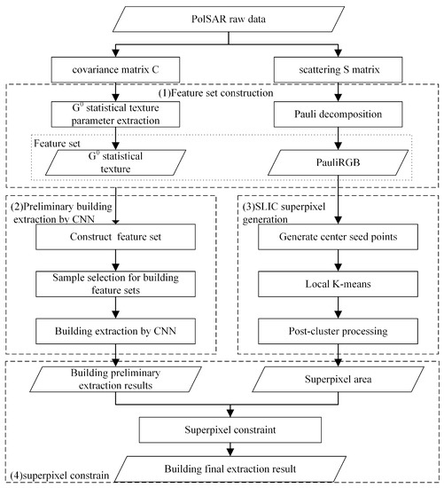
Figure 1.
Flow chart of building extraction based on CNN and superpixel in the PolSAR image.
2.1. Building Feature Set Extraction from SAR Image
PolSAR images have abundant polarization information and texture information for building feature extraction. Therefore, this part introduces the PauliRGB features used to describe the polarization information and the G0 statistical texture parameters used to describe the polarization statistical texture information, which form the feature set extracted by the building.
In general, the electromagnetic scattering of a radar target can approximate a linear process. After determining the scattering space coordinate system and its corresponding polarization basis, there is a linear transformation relationship of the polarization components between the radar emission wave and the target scattering echo. The scattering process of the target can be represented by a complex matrix, which is the Sinclair S matrix, as follows [27]:
where and represent the co-polar scattering components, and and represent the cross-polar scattering components. In the monostatic case, the two cross-polar components are equal, i.e., .
In the actual analysis of PolSAR data, the polarization covariance matrix C is introduced to describe the dynamically changing environment and objectives. Covariance matrix C can be written as:
2.1.1. PauliRGB
The scattering S matrix is expressed by Pauli decomposition as the complex sum of the Pauli matrices. The scattering S matrix is associated with each basis matrix, with
where are all complex and are given by the following:
The Pauli decomposition of deterministic targets consists of four scattering mechanisms. The first scattering mechanism is a single scattering from a plane surface. The second and third are double or even bounce scattering from corners with a relative orientation of and , respectively. The final scattering mechanism is all the antisymmetric components of the scattering S matrix.
In the monostatic case, the Pauli matrix basis can be simplified to the first three matrices and = 0. The power of the three matrices can be described as follows:
Generally, buildings are dominated by double scattering. Buildings with orientation angles have strong double scattering. Non-buildings mainly include rivers, roads, and bare land, with odd-level scattering and other types of scattering. The vegetation scattering mechanism is more complicated than other non-building phenomena. The vegetation’s power in Pauli decomposition is similar to the buildings, which have an orientation angle.
2.1.2. G0 Statistical Texture Parameter
To better simulate extreme heterogeneous regions in SAR images, Freitas [28] proposed the G0 distribution. It models texture variables using an inverse gamma distribution based on the multiplicative model. The uniformity of the target can be reflected by the texture parameter of the G0 distribution [29]. This parameter can provide valid information in building extraction.
For non-uniform regions, the texture features of the object target have a wealth of available information. The SAR image uses the multiplicative model to model it. The SAR images can be expressed as multiplicative products of mutually independent texture variables and speckle variables :
where Z represents SAR image data. It may be an intensity image, an amplitude image, a covariance matrix, or a coherence matrix. represents the texture variable, reflecting the average backscattering coefficient of the scatters in the ground-resolving unit. It models the inverse gamma () distribution for heterogeneous regions, for example, urban areas. represents the speckle of the SAR image, which obeys the gamma distribution for the L-look single-polarimetric SAR intensity image [30] and the Wishart distribution for the L-look multi-polarimetric SAR image [31]. According to Equation (11), the SAR image obeys the G0 distribution, and the probability density distribution of the L-look multi-polarimetric SAR image is
where is the texture parameter, is the scattering vector dimension, is the gamma function, , is the mean, and is the trace of the matrix.
Regarding the G0 texture parameter estimation of L-look multi-polarimetric SAR data, according to the study of Khan [32], we can make . Then, the th moments of can be uniformly expressed as
Doulgeris [33] estimates the texture parameter of the G0 distribution for multi-polarimetric SAR image by using the second-order moment of M.
According to , the estimation formula of the G0 distribution texture parameter of the multi-polarimetric SAR image can be expressed as
where .
The range of calculated using Equation (15) is usually too broad, which inconveniences the display of images and the statistics of samples. For this reason, this paper takes the logarithm operation as a new statistical texture feature named G0-para
2.2. Preliminary Building Extraction by CNN
First, we select the training sample and verification sample sets, count the number of building pixel points in the true ground map of the image, and select the positive training sample by random. Additionally, we select the same number of non-building negative samples in the non-building area. The test sample set, identical to the total number of training samples, is selected from the unselected samples. For the construction of a single sample, the pixels are selected and taken as the sample center, and then the range of size N × N is selected as the sample. Second, the acquired samples are input to the convolutional neural network. After the training is sufficient, we use the fitted model to extract the building. The learning ability of convolutional neural networks enables the use of contextual information in PolSAR images. The model of PolSAR building extraction under the convolutional neural network is obtained after training. It will be used to extract the building.
2.2.1. Convolution Layer
Each convolutional layer can obtain multiple feature maps, and generating one feature map includes two processes: convolution and nonlinear activation. The convolution process consists of two parts, the convolution kernel and a bias parameter, which are shared during the generation of a featured image [34]. For an N-channel image of size W×H, using a two-dimensional convolution kernel of size , the convolution calculation at is as follows:
where (ii, jj) is the result of the value obtained by the kth convolution kernel, (i, j) is the pixel value of the (i,j) position of the n channel, and (p,q) is the filter kernel (p,q) the weight of the position, is the weight value of the kth convolution kernel, and is the stride of the convolution kernel movement. The size of the obtained feature map is .
The nonlinear activation process enhances the nonlinear characteristics [34]. It is necessary to use a nonlinear activation function. The process takes as an input. It is activated by a nonlinear function to obtain an activation value, which constitutes the final feature image. The specific formula is as follows:
where the nonlinear activation function f(∙) is in many forms, such as sigmoid, tanh, and ReLU. Because the ReLU function can better solve the gradient disappearance problem in the training process compared to other activation functions, it can make the network sparse, reduce the parameter interdependence, and alleviate the over-fitting problem [35]. Therefore, we use the ReLU function as the nonlinear activation in this paper. Its expression formula is as follows:
2.2.2. Pooling Layer
The pooling layer summarizes the features of the convolution by downsampling, thereby expanding the receptive field while reducing the computational complexity in the training process [36]. The pooling operation allows the same result even if the image features have a small translation or rotation. Usually, the pooling operation involves maximum pooling and average pooling. This paper uses the maximum pooling operation, taking as input, using the size of the pooling window and the stride size . The pooled output value is . The calculation process is as follows:
The resulting pooled result size is .
2.2.3. Fully Connected Layer
After the convolution and pooling layers are superimposed several times to obtain the feature image, the output feature map needs to be compressed into a one-dimensional vector. The fully connected layer can integrate high-dimensional features obtained by the convolutional layer and pooling layer. The fully connected layer maps the input dataset to the output set by feed-forward mode, and each neuron is fully connected to all neurons in its previous layer. The output of each node is a weighted unit, followed by a nonlinear activation function to distinguish those that are not linearly separable [37]. Taking as the input and as the output of the layer, the calculation process is as follows:
where is the weight matrix, is the offset matrix, and is the activation function. The activation function is the ReLu function. Softmax is used in the final output classification result so that the output probability value is between 0 and 1 and the sum is 1.
2.3. SLIC Superpixel Generation and Superpixel Constraint
A superpixel region is a collection of spatially contiguous pixels with similar characteristics that maintain similar ground boundary contours. Superpixels are often used in the pre-processing steps of image information extraction. In the field of image classification, it can be considered that all pixels in a superpixel belong to the same category. Then, superpixel classification is utilized to reduce noise interference in an image. Speckle noise is an important factor that affects the classification accuracy of PolSAR images. In recent years, superpixel-based classification methods have achieved better classification effects in PolSAR images [38,39].
2.3.1. SLIC Superpixel Generation
This paper uses the SLIC algorithm to obtain superpixels from PolSAR images. Considering that the target decomposition parameter is an important feature for describing the class information, the three components of the Pauli decomposition have obvious physical meaning. Therefore, the PauliRGB is used to replace the spectral features in the traditional optical image. The main details of the processing steps are as follows:
- Generate center seed points: Firstly, we generate a PauliRGB gradient image. Secondly, select the seed point as the initial center of the superpixel according to the step S sampling. Finally, adjust the seed point to the lowest point of the gradient image in the local S ∗ S range;
- Local K-means: First, the distance of each pixel to the center of the superpixel is calculated in the range of 2S ∗ 2S of each superpixel center and divide the pixel into the nearest superpixel. Second, SLIC’s search scope is limited to 2S ∗ 2S, which speeds up algorithm convergence. The distance between two pixels is measured in d. Third, we assume that the Pauli decomposition feature vectors of pixel (, ) and pixel (, ) are (,,) and (,, ). The computational formula of spatial distance, Pauli distance, and distance d is defined as follows:After the calculation, we update the center of each superpixel. Next, we repeat the above steps until convergence or it reaches the maximum number of iterations. Finally, a superpixel of approximately S ∗ S size can generate;
- Post-cluster processing: The superpixels with less than a certain number of pixels are merged into the nearest superpixel to obtain the final PolSAR superpixel image.
2.3.2. Superpixel Constraint
For PolSAR images, the target decomposition parameters are an important feature to describe ground information. The Pauli decomposition’s three components have obvious physical significance, representing odd scattering, dihedral angular scattering, and π/4 even scattering, respectively. Meanwhile, a PauliRGB composite image is the standard display mode of PolSAR images. Therefore, in this paper, Pauli features are used to replace spectral features in traditional optical images.
Aiming at the effect of speckle noise in PolSAR data on building extraction and the over-smoothing phenomenon caused by CNN, a superpixel constraint method based on the CNN classification result is proposed to extract buildings more accurately. After obtaining the superpixel area and the preliminary extraction area of the building, we modify the building area with the superpixel constraint. First, the extracted results in the same superpixel area are counted. For the statistical results, if the number of buildings in the statistics is less than the number of non-buildings, the buildings in the superpixel will be classified as non-buildings; otherwise, the pixels in the superpixel will not be modified.
3. Experiment and Results
In order to prove the effectiveness of the method, three different PolSAR sensors are adopted, including E-SAR, GF-3, and RADARSAT-2. In the case of a convolutional neural network using the same sample and the same structure and training mode, we compare the results of our method with those of other methods. Further, we also compare the convolutional neural network method for PolSAR classification and the method we propose. In this section, the experimental data, experimental sample construction, and training patterns are described, and the experimental results are illustrated.
3.1. Study Area and Data Set
Three different study areas and data sets are used in this paper. The optical images of Figure 2(a2,b2,c2) are from Google Earth. Figure 2(a3,b3,c3) is the true ground map, which is derived from the distribution vector of buildings and the interpretation of optical remote sensing images taken at the same time.
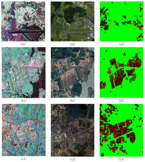
Figure 2.
The SAR and optical images, and the true ground map. (a1,b1,c1) are the PauliRGB images from E-SAR, GF-3, and RADARSAT-2, respectively. (a2,b2,c2) are the optical images. (a3,b3,c3) are the true ground map. Red is the building and green is the non-building in (a3,b3,c3).
The first study data were obtained by E-SAR. E-SAR is an experimental SAR developed in Germany with optional vertically polarized or horizontally polarized antennas. We conducted experiments using the airborne L-band fully polarimetric E-SAR data of Oberpfaffenhofen, Germany, obtained in July 1999. The azimuth of the image has been conducted with 2-look processing; the image size is pixels; and the azimuth resolution and ground resolution are both about 3 m. The image mainly includes land types such as buildings, woodlands, farmland, and roads. The E-SAR image and the real surface are shown in Figure 2(a1,a3).
The second study data were obtained by GF-3. GF-3 is a C-band SAR satellite platform developed by China. This study used PolSAR data acquired on 9 December 2016 in Huashan, Wuhan, China. The GF-3 image size is pixels, which means that the azimuth resolution and ground are both about 8 m. The image and the real surface are shown in Figure 2(b1,b3). The third study’s data was obtained by RADARSAT-2. RADARSAT-2 is a C-band SAR satellite platform developed in Canada. This study uses PolSAR data acquired on December 7, 2011, in Wuhan, China. The image size is 450 × 550 pixels, the azimuth resolution is 5 m, and the ground resolution is 4.7 m. The image and the real surface are shown in Figure 2(c1,c3).
3.2. Sample Construction and Network Parameters
In the extraction of PolSAR buildings, the use of CNN to achieve the extraction of buildings, the construction of training samples, and the initialization of convolutional neural network parameters are essential for the effective acquisition of the model for PolSAR building extraction.
In the construction of the sample, we used the real surface map to select the building as a positive sample and the non-building as a negative sample. For the selection of positive samples, we selected 15% of the building area pixels randomly as the center point of the sample. For the selection of negative samples in the non-building area, we randomly selected the same number of pixels as the positive sample as the center point of the sample. We used these pixels as the center point of the sample. After that, a window of size N × N was constructed, centering on the selected pixel point, and the data in the window were taken as a sample, and the size of the sample is , where C is the number of channels. The label value corresponds to the category of the central pixel point. After an experimental analysis, the sample map size of ESAR data were selected as pixels, and the sample map size of RADARSAT-2 and GF-3 data were selected as pixels. See Section 4.2.2 for details.
To learn the higher-level features of the feature set in the sample while extracting the building, we use a CNN. The CNN that we construct is a Lenet5-like network, shown in Figure 3, which is a relatively simple convolutional neural network. The structure includes two convolutional layers, two pooling layers, and two fully connected layers, wherein the convolutional layer has several convolution kernels of 500 and 100, respectively. The number of fully connected layers is 200 and 84, respectively. The size of the convolution kernel is pixels, and the size of the pooled layer is pixels. The stride size is 1 pixel. The initialization of all parameters in the network selects randomly from a Gaussian distribution with a variance of 1. In addition to the bias parameter, the initialization of the bias parameter is zero. In the convolutional neural network training, we used 500 training samples as one batch, and the learning rate during training was 0.01. In training, the loss value is less than 0.005 as a complete fit, and the model can be acquired for subsequent building extraction.
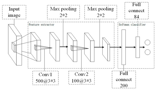
Figure 3.
The convolutional neural network structure for building extraction.
3.3. Building Extraction Results and Analysis
For the three different PolSAR images, we extracted the buildings based on our method and five other methods separately. The five other methods include: using feature extraction and an eigenvalue-based method [12] and using the support vector machine (SVM) classifier [40] by using the feature set we propose for building detection, real vector representation tailored for Convolutional Neural Network (RVCNN) [20], Polarimetric-Feature-Driven Convolutional Neural Network (PFDCNN) [21], the proposed CNN of PauliRGB and G0, and the method of adding superpixel constraints on this basis. The SVM classifier kernel is a radial basis function, the gamma coefficient is 0.2, determined by the number of channels, and the penalty parameter is 200. The RVCNN method inputs the normalized six-dimensional real feature vector, which contains the coherence or covariance matrix of multi-looked PolSAR data, into the four-layer convolutional neural network for PolSAR classification. The PFDCNN uses classical roll-invariant polarimetric features and hidden polarimetric features in the rotation domain to drive the proposed deep CNN model. The samples used for the experiments are consistent, whether it is a different CNN, SVM, or eigenvalue-based method.
For the evaluation of accuracy, we use the accuracy rate (AR), the false alarm rate (FAR), and the F1-score [41] for the harmonic evaluation of the detection rate and false alarm rate. Among them, the accuracy rate is the correct proportion of the number of building pixels in the real building, and the false alarm rate is the number of non-building pixels in the extracted building. The F1-score is a way of combining the precision and recall of the model, and it is defined as the harmonic mean of the model’s precision and recall. What is more, the CNN training samples are not excluded for the calculation of AR, FAR and F1-score.
3.3.1. ESAR
For the extraction of buildings from ESAR data, the buildings with large dip angles are very similar to the vegetation, and the parking lot with vehicles is similar to the buildings. The building extraction results of the six methods are shown in Figure 4.
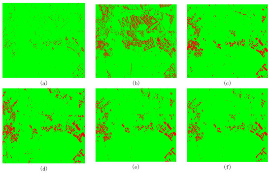
Figure 4.
ESAR image building extraction results. (a) Quan’s threshold extraction method; (b) PauliRGB and G0 statistical texture parameters using SVM results; (c) RVCNN; (d) PFDCNN; (e) PauliRGB and G0 Statistical texture parameters using CNN; (f) as the result of introducing superpixel constraints in (e).
In the ESAR data experiment results, it shows that the method using CNN is more effective than other methods. The CNN can accurately determine the location of the building. In the SVM method, vegetation is easily misclassified as a building because it has a similar scattering mechanism to buildings with large orientation angles. The method of using thresholds to extract buildings from the image is not effective. For all methods using CNN, the proposed method has a relatively high accuracy for the extraction of buildings, and the false alarm rate of it is lower than that of other non-CNN methods. In terms of details, the method proposed by us can extract large-angled buildings and suppress the interference of parking lots, which have a regular arrangement of vehicles. The accuracy comparison is shown in Table 1.

Table 1.
Different methods of building extraction effects under ESAR data.
3.3.2. GF-3
For the extraction of buildings in GF-3 data, the buildings include relatively high residential buildings, individually distributed villas, houses under construction, and large single-unit buildings. Non-buildings include vegetation, water, roads, bare soil, etc. The building extraction effect is shown in Figure 5.
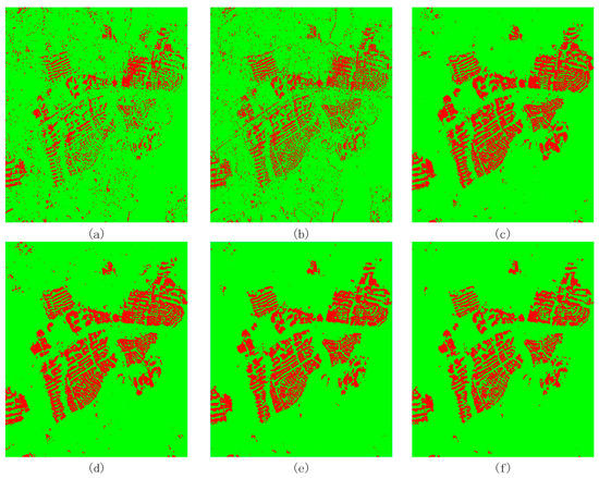
Figure 5.
GF-3 image building extraction results. (a) Quan’s threshold extraction method; (b) PauliRGB and G0 statistical texture parameters using SVM results; (c) RVCNN; (d) PFDCNN; (e) PauliRGB and G0 Statistical texture parameters using CNN; (f) as the result of introducing superpixel constraints in (e).
From Table 1, the extraction accuracy rate and false alarm rate of the building using the three methods of the CNN are better than the methods of using the SVM method and the threshold to obtain buildings. Among the three methods using CNN, our proposed feature set and method for building extraction can better extract buildings, including the control of the boundary of the building and the suppression of false alarms. In terms of details, the method proposed by us can have a better suppression effect on non-buildings, such as streetlamps on the side of the road than other CNN methods. The accuracy comparison is shown in Table 2.
Table 2.
Different methods of building extraction effects under GF-3 data.
From Table 2, we can see that the accuracy of the building extraction is higher in the three methods using CNN. The proposed method with the selected feature set can have higher building extraction accuracy and a lower false alarm rate than the comparison methods in building extraction. In the case of high accuracy in building extraction, the false alarm rate is reduced by about 11%, and the F1-score is increased by more than 6.7% by the proposed method.
3.3.3. RADARSAT-2
The buildings in this data image mainly include factory buildings, residential buildings, and tall buildings. Non-buildings include forests, vegetation, roads, and railways. Among them, roads and railways have many similarities to buildings in terms of the scattering mechanism and spatial structure, which have a significant influence on the extraction of buildings. The building extraction results under different methods are shown in Figure 6.
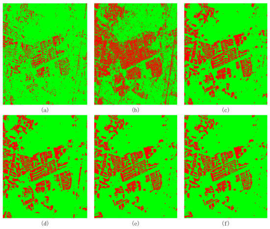
Figure 6.
RADARSAT-2 image building extraction results. (a) Quan’s threshold extraction method; (b) PauliRGB and G0 statistical texture parameters using SVM results; (c) RVCNN; (d) PFDCNN; (e) PauliRGB and G0 Statistical texture parameters using CNN; (f) as the result of introducing superpixel constraints in (e).
The three methods using CNN have resulted in a significant improvement in the overall extraction of the building, and the accuracy of the outlines and targets of the building has also improved. In the method of using convolutional neural networks, the feature sets, and methods we use can make the railways and highways better differentiated from buildings than the other two methods. There is still the phenomenon that some railways are mistakenly divided into buildings in the experiment. In detail, our approach can more accurately describe the boundary of the building. The building extraction accuracy is shown in Table 3.
Table 3.
Different methods of building extraction effects under RADARSAT-2 data.
From the experimental results of three different types of data, the proposed method can improve the extraction effect of buildings compared to other methods. The main improvement is the suppression of false alarm rates in building extraction. This method can distinguish buildings from similar buildings. In the case of the building extraction accuracy rate, the false alarm rate has been reduced by at least 12%, and F1 has increased by more than 7%.
4. Discussion
4.1. Method Characteristic Analysis
In this section, we analyze the characteristics of this method in three aspects. Firstly, the advantages of the combination of the polarization feature and the statistical texture feature are discussed. Furthermore, we compare the effects of using a single feature and multiple features in the same way. Secondly, the ability of CNN to utilize the spatial information of polarimetric SAR building is analyzed. In the case of the same features, we use CNN and multi-layer perceptrons (MLP), respectively, to extract PolSAR buildings and then compare the accuracy of their results. Finally, the effect of applying superpixels is discussed on the accuracy of the results. By keeping the characteristics and methods unchanged, the effects of using a superpixel constraint on the accuracy of the results are compared.
4.1.1. Combination of Polarization and Statistical Features
PauliRGB is the most basic and commonly used method for characterizing PolSAR. However, using only PauliRGB to learn building features can only train the optimal feature information of buildings in PauliRGB images. In this case, the information in the PolSAR image is not sufficient. Further, there are some targets in PauliRGB images that are similar to the scattering mechanism and spatial structure of buildings. In the case of using only PauliRGB, they are easy to mistakenly divide into buildings, such as the parking lot, the street tree, etc., as shown in Figure 7.
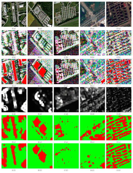
Figure 7.
Buildings and similar building features in the PolSAR image (A,B,C) images from ESAR. Group (D) images from GF-3 and Group (E) images from RADARSAT-2. Where (a) is the optical image, (b) is PauliRGB, (c) is the mask of the real building distributed on PauliRGB (red area), and (d) is the G0 statistical texture parameter. (e) Classification results obtained by using only PauliRGB as CNN input training, in which red is a building, green is a non-building, and (f) is a classification obtained by adding a G0 statistical texture parameter to PauliRGB as a CNN input training, in which red is a building and green is a non-building.
As unique and vital information in PolSAR data, statistical information can describe the heterogeneity of PolSAR. The statistical texture parameters can be used to interpret the statistical information of PolSAR features. The building area appears as a heterogeneous area in PolSAR. The different arrangement of the buildings results in different textures. In PolSAR images, the scattering mechanisms of different components of the same building may be different, so the building area contains essential context information. In view of the above situation, the G0 distribution model can apply uniformly to them and contribute to building extraction.
Furthermore, the use of CNN for PolSAR data classification has demonstrated that the introduction of appropriate features affects the classification of PolSAR. Through the G0 statistical texture parameters under different data in the Figure 7c group, the G0 statistical texture parameters can strengthen the characteristics of buildings and weaken the non-building features of buildings, such as the building features in Figure 7(A(d),B(d),E(d)) are enhanced, the street tree features in Figure 7 (B(d),D(d)) are adequately distinguished, and in C(d) and D(d), neatly arranged cars in the parking lot and roads, their differentiation from buildings has enhanced. Therefore, we add the G0 statistical texture parameter to the input of CNN based on PauliRGB. The building extraction results are shown in Figure 7b,e,h. Combined with Figure 7 and Figure 8, the introduction of G0 statistical texture parameters on PauliRGB can improve the building extraction effect. By comparing the two groups in (e,f) of Figure 7, the outlines of the buildings in A(f) and E(f) become more accurate, and the results of the extraction are less misclassified. The street trees in B(f) and D(f) with similar spatial structures of buildings are more accurately distinguished, and the cars on the parking lot where the parts of C(f) had a misclassified result are accurately classified. According to the overall results in Figure 8, after adding the G0 statistical texture parameters, the building extraction results of the three data indicate that the accuracy of the building profile is improved, the misclassification phenomenon is improved, and the non-building can be effectively distinguished, which has a similar scattering mechanism and spatial structure to buildings.
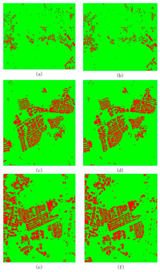
Figure 8.
Comparison of feature sets under three data using G0 texture parameters before and after comparison. (a,b) is the experimental result under ESAR data, (c,d) is the experimental result under GF-3 data, and (e,f) is the experimental result under RADASAT-2 data. Where (a,c,e) is the experimental result of the input of only PauliRGB and (b,d,f) is the experimental result of the input texture parameter of PauliRGB and G0.
Combined with Table 4, we find that after using the G0 statistical texture parameters, the false alarm rate reduced by at least 5% and the evaluation parameter F1 increased by about 5% when the accuracy improved. Therefore, combining PauliRGB and G0 statistical texture parameters can improve the extraction of buildings using CNN.
Table 4.
Building extraction accuracy table using G0 statistical texture parameters.
4.1.2. CNN’s Use of Spatial Information
The convolutional layer and the pooled layer are used alternately to simulate the working model of the human cerebral cortex through convolution and weight sharing. The deep features of the input target are learned and acquired, and the perception domain of the network is expanded, thereby fully utilizing the spatial features. Therefore, convolutional neural networks, as a classifier with a deep architecture, can reveal the deep features in buildings in PolSAR images where shallow layers’ features cannot be found.
To verify that convolutional neural networks can effectively apply spatial information to PolSAR buildings, we use convolutional neural networks to compare the use of multilayer perceptrons (MLP) for PolSAR building extraction. The difference between MLP and CNN is that the MLP is composed of a fully connected layer, and there is no convolution layer or pooling layer. The MLP cannot expand the receptive field and make full use of the spatial characteristics. We use a four-layer MLP with neurons of 500, 350, 200, and 84, using the feature set of PauliRGB and G0 statistical texture parameters as input. The MLP and CNN building extraction effects are compared, and the results of that are shown in Figure 9.
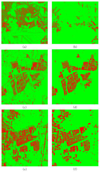
Figure 9.
Comparison of using the MLP and CNN methods. (a,b) is the experimental result under ESAR data, (c,d) is the experimental result under GF-3 data, and (e,f) is the experimental result under RADASAT-2 data. Where (a,c,e) is the experimental result of the MLP and (b,d,f) is the experimental result of the CNN.
After using CNN to learn the spatial information of the building and obtain deeper features, the extraction effect of the building improves, the phenomenon of misclassification is reduced, and the outline of the building becomes accurate. In Table 5, compared with the use of MLP, the accuracy of CNN for building extraction increased by about 13%, the false alarm rate decreased by at least 17%, and the F1 parameter increased by at least 17%.
Table 5.
Building extraction accuracy table using the MLP and CNN methods.
4.1.3. Effect Analysis of Superpixel
Speckle is a unique scattering phenomenon of PolSAR images. Speckles increase the difficulty of image interpretation and reduce the performance of image segmentation and classification. In the extraction of PolSAR buildings, due to the influence of the speckles, many non-buildings are mistakenly extracted into buildings. The superpixel algorithm aggregates pixels into area units of roughly uniform size. Reasonable superpixels are conducive to overcoming the interference of speckle noise in PolSAR images.
Considering that the distribution of buildings on the earth’s surface cannot be a scattered distribution of single pixels, we apply superpixel constraints to the building of PolSAR imagery. The core idea of the superpixel constraint is to filter the building extraction results by using each superpixel region and to filter out the scattered extraction results. From Figure 10b,d,f, the scattered misclassification results are corrected while maintaining the outline of the building after the introduction of superpixels. In Table 6, after using the superpixel constraint, the accuracy of the building extraction result decreases slightly, the false alarm rate decreases significantly, and the evaluation parameter F1 increases from 2% to 4%. Therefore, the introduction of superpixels can provide better adaptability and usability for the extraction of buildings under PolSAR.
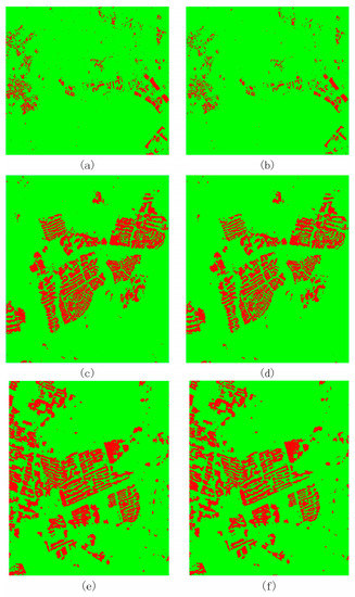
Figure 10.
Comparison of results before and after superpixel constraints under three data. (a,b) is the experimental result under ESAR data; (c,d) is the experimental result under GF-3 data; and (e,f) is the experimental result under RADASAT-2 data. (a,c,e) are experimental results without superpixel constraints and (b,d,f) are experimental results after using superpixel constraints.
Table 6.
Building extraction accuracy table using the superpixel methods.
In this paper, the feature set of PauliRGB and G0 statistical texture parameters is used as the input to CNN. It combines polarization information and the unique statistical texture information of the building under the PolSAR image, which improves the information utilization rate of the building and makes the building’s extraction more accurate. The use of CNN to fully dig out building information in PolSAR images significantly improves building extraction. The introduction of superpixel segmentation optimizes the building extraction accuracy and makes the building contour boundary more accurate.
4.2. Parameter Impact Analysis
In the experiment of classifying PolSAR features using CNN, different parameters have an impact on the accuracy of feature classification. In the building extraction experiment of this paper, many factors that have an impact on building extraction are found, including different sample selection methods, different training samples in the total building pixel ratio, and different sizes as CNN inputs. We discuss them in this section.
4.2.1. Discussion of Sample Selection
In deep learning, the selection structure of the sample and the universality of the sample are necessary for the trained model. Our sample selection method is different from the sample selection method for convolutional neural networks for PolSAR image classification. Generally, in the classification of PolSAR features by CNN, it is mainly to use the real surface map to select samples for each type of ground object for training and the remaining as the test sample set. The final evaluation in this method is similar to the test sample set. The number of buildings in the real object distribution is significantly less than that of other non-building objects, and the proportion of similar buildings in the PolSAR image is less than that of the non-building objects. We propose to randomly select the building elements using the buildings in the real surface map and select the training samples of N and the test samples of N. Then, for the non-building area, we select a specific non-building area instead of all non-building areas, and randomly select a number N of non-building training samples and a number N of test samples in the non-building area.
Under this method, we use fewer training samples than under other CNN classification methods. It increases the proportion of non-building land types with similar buildings in the training sample in all non-buildings. By increasing the training frequency of the object samples that are easily misclassified, the convolutional neural network model can learn a useful PolSAR building identification model at a relatively small cost. The building extraction effect under different sample selection methods is shown in Figure 11, and the results are not superpixel-constrained. Through the graphical representation of the two samples, we can see that the trained model is more focused on distinguishing non-buildings similar to buildings by increasing the utilization of non-building samples in the training sample. This process improves the accuracy of building extraction, and the description of the boundary of the building is more accurate than before.
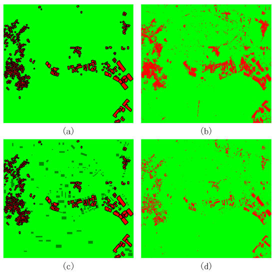
Figure 11.
Sample selection and building extraction results. (a) is the samples from the true surface map; (b) is the result of building extraction using (a) samples; (c) consists of positive and negative samples (dark green); and (d) is the result of building extraction using (c) samples.
4.2.2. Different Image Block Sizes on Building Extraction
Using image blocks as input and CNN to learn depth features shows strong recognition ability, but the ability has certain defects in space segmentation. Over-smoothing of the boundary often occurs in the classification results, and it is easy to cause smaller targets to be ignored. Although a certain degree of excessive smoothing of the edges can be understood and accepted. Additionally, the use of the minimum adaptive map for CNN can slightly slow down the smoothing phenomenon [42]. However, we find that the use of small image block sizes during building extraction is not the best for building extraction, so we test the size of the image blocks.
In this paper, we use three different types of PolSAR data. For different data, we select different-sized samples in the same position as the input of CNN. Here we will discuss the effect of different speckle sizes on building extraction, and the results are not superpixel-constrained. The building extraction evaluation index F1 size under different sizes is shown in Figure 12.
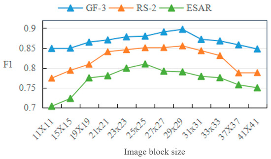
Figure 12.
Accuracy of building extraction results under different image block sizes.
We have found that a large image block size will lead to the occurrence of serious over-smoothing, resulting in poor extraction of the building. Too small a pattern will also lead to a decrease in extraction accuracy. It can be seen from the figure that, under the three-image data, the scale has an outstanding building extraction result of 25 × 25 pixels to 29 × 29 pixels. The size of the sample spots under GF-3 and RADASAT-2 images is suitable for 29 × 29 pixels. The size of the sample spots under ESAR images is 25 × 25 pixels. At this scale, the boundary smoothing phenomenon has a good balance with the building extraction accuracy.
4.2.3. The Size of Different Training Samples on Building Extraction
The number of building training samples is significant for the training of CNN. Too few building training samples will lead to insufficient robustness of the model, resulting in a high rate of missed detection of the final building extraction results. Conversely, too many building training samples can lead to high training costs in model training, which is undesirable in the application. Therefore, we tested the ratio of the number of pixel points in the building training sample to the number of total building pixel points and gave the final training sample ratio through experiments.
In this paper, we use the three different types of PolSAR sensor data. For different types of data, we select different proportions of samples as the input of CNN. By comparing the building extraction results at different scales, we obtain the sample ratio we need. The building extraction accuracy of the three data sets increases as the proportion of the training samples increases, as shown in Figure 13. After the selection ratio reaches 15%, the extraction accuracy of the building tends to be gentle with the increase of the sample proportion, and even a slight decrease. It shows that the increase in the number of building samples has improved the extraction effect of the building, but the data redundancy caused by the excessive number of training samples does not significantly help the extraction effect. Taking into account the real distribution factors of the building and the cost factor of the training model, we selected 15% of the building elements in the real building as training samples for all three types of data.
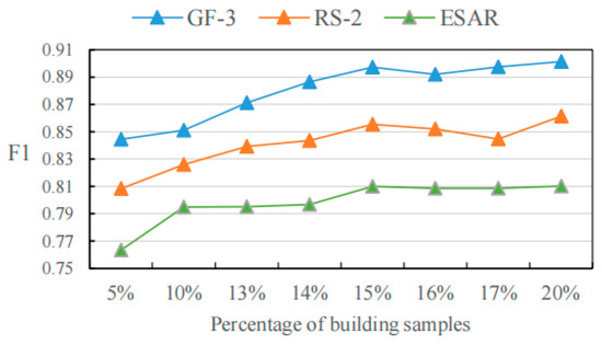
Figure 13.
Building elements used for training account for the accuracy of building extraction results at different percentages of all building pixels.
5. Conclusions
This paper proposes a method for building extraction with multi-features using convolutional neural networks and superpixels for PolSAR images. G0 statistical texture parameters and PauliRGB in the proposed method are used as a new feature set as input to CNN for training. The combination of polarization features and statistical texture features can reduce the influence of other classes with the same spatial structure as the building on the building extraction results. The superpixel constraint applied to the preliminary results decreases the effect of noise, optimizes the boundary of building extraction results, reduces the appearance of false alarms, and improves the overall effect of building extraction.
In this paper, we use the PolSAR data from ESAR, GF-3, and RADASAT-2 sensors for experimental verification. The F1 parameter of building extraction accuracy is improved by at least 6%. The false alarm rate is reduced by at least 10% when the building extraction accuracy is comparable, which proves that our method is more suitable for the extraction of PolSAR buildings. After using the G0 texture parameter, F1 is increased by about 5%. Furthermore, after the superpixel constraint, the evaluation parameter F1 increases by 2% to 4%. The proposed method achieved better building extraction results using CNN and superpixel with G0 statistical texture and polarization features from PolSAR images.
For instance, there are still some misclassifications in some cases, such as the edge error phenomenon and small house erasure phenomenon caused by the introduction of CNN, and the incomplete phenomenon of the building caused by different scattering mechanisms in different parts of the building. At present, deep learning requires a large amount of data, but the amount of data used in PolSAR building extraction is limited. More data can be used for support in the future.
Author Contributions
Q.C. provided the thought. M.L. and Q.S. wrote the manuscript; M.L. supervised, edited, restructured; Q.C., M.L., Q.S., Y.X. and X.L. professionally optimized the manuscript; Q.C. acquired the funding. All authors have read and agreed to the published version of the manuscript.
Funding
This research was funded by the National Natural Science Foundation of China (NSFC), grant number 41771467.
Data Availability Statement
Not applicable.
Acknowledgments
The authors would like to thank the funding and support from the China University of Geosciences, which we gratefully appreciate.
Conflicts of Interest
The authors declare no conflict of interest.
References
- Du, P.; Samat, A.; Waske, B.; Liu, S.; Li, Z. Random forest and rotation forest for fully polarized SAR image classification using polarimetric and spatial features. ISPRS J. Photogramm. Remote Sens. 2015, 105, 38–53. [Google Scholar] [CrossRef]
- Li, X.; Guo, H.; Zhang, L.; Chen, X.; Liang, L. A new approach to collapsed building extraction using RADARSAT-2 polarimetric SAR imagery. IEEE Geosci. Remote Sens. Lett. 2012, 9, 677–681. [Google Scholar]
- Xiang, D.; Tang, T.; Ban, Y.; Su, Y.; Kuang, G. Unsupervised polarimetric SAR urban area classifification based on model-based decomposition with cross scattering. ISPRS J. Photogramm. Remote Sens. 2016, 116, 86–100. [Google Scholar] [CrossRef]
- Niu, X.; Ban, Y. Multi-temporal RADARSAT-2 polarimetric SAR data for urban land-cover classification using an object-based support vector machine and a rule-based approach. Int. J. Remote Sens. 2013, 34, 1–26. [Google Scholar] [CrossRef]
- Xiang, D.; Ban, Y.; Su, Y. Model-Based Decomposition With Cross Scattering for Polarimetric SAR Urban Areas. IEEE Geosci. Remote Sens. Lett. 2015, 12, 2496–2500. [Google Scholar] [CrossRef]
- Lee, J.S.; Grunes, M.R.; Kwok, R. Classification of multi-look polarimetric SAR imagery based on complex Wishart distribution. Int. J. Remote Sens. 1994, 15, 2299–2311. [Google Scholar] [CrossRef]
- Deng, L.; Wang, C. Improved building extraction with integrated decomposition of time-frequency and entropy-alpha using polarimetric SAR data. IEEE J. Sel. Top. Appl. Earth Obs. Remote Sens. 2013, 7, 4058–4068. [Google Scholar] [CrossRef]
- Xu, Q.; Chen, Q.; Yang, S.; Liu, X. Superpixel-Based Classification Using K Distribution and Spatial Context for Polarimetric SAR Images. Remote Sens. 2016, 8, 619. [Google Scholar] [CrossRef]
- Chen, Q.; Yang, H.; Li, L.; Liu, X. A Novel Statistical Texture Feature for SAR Building Damage Assessment in Different Polarization Modes. IEEE J. Sel. Top. Appl. Earth Obs. Remote Sens. 2019, 13, 154–165. [Google Scholar] [CrossRef]
- Ping, J.; Liu, X.; Chen, Q.; Shao, F. A Multi-scale SVM-CRF Model for Buildings Extraction from Polarimetric SAR Images. Remote Sens. Technol. Appl. 2017, 32, 475–482. [Google Scholar]
- Zhai, W.; Shen, H.; Huang, C.; Pei, W. Fusion of polarimetric and texture information for urban building extraction from fully polarimetric SAR imagery. Remote Sens. Lett. 2016, 7, 31–40. [Google Scholar] [CrossRef]
- Quan, S.; Xiong, B.; Xiang, D.; Zhao, L.; Zhang, S.; Kuang, G. Eigenvalue-Based Urban Area Extraction Using Polarimetric SAR Data. IEEE J. Sel. Top. Appl. Earth Obs. Remote Sens. 2018, 11, 458–471. [Google Scholar] [CrossRef]
- Pellizzeri, T.M. Classification of polarimetric SAR images of suburban areas using joint annealed segmentation and “H/A/α” polarimetric decomposition. ISPRS-J. Photogramm. Remote Sens. 2003, 58, 55–70. [Google Scholar] [CrossRef]
- Yan, L.; Zhang, J.; Huang, G.; Zhao, Z. Building Footprints Extraction from PolSAR Image Using Multi-Features and Edge Information. In Proceedings of the 2011 International Symposium on Image and Data Fusion, Tengchong, China, 9–11 August 2011. [Google Scholar]
- Deng, L.; Yan, Y.; Sun, C. Use of Sub-Aperture Decomposition for Supervised PolSAR Classification in Urban Area. Remote Sens. 2015, 7, 1380–1396. [Google Scholar] [CrossRef]
- Wurm, M.; Taubenbck, H.; Weigand, M.; Schmitt, A. Slum mapping in polarimetric SAR data using spatial features. Remote Sens. Environ. 2017, 194, 190–204. [Google Scholar] [CrossRef]
- De, S.; Bruzzone, L.; Bhattacharya, A.; Bovolo, F.; Chaudhuri, S. A Novel Technique Based on Deep Learning and a Synthetic Target Database for Classification of Urban Areas in PolSAR Data. IEEE J. Sel. Top. Appl. Earth Obs. Remote Sens. 2018, 11, 154–170. [Google Scholar] [CrossRef]
- Bi, H.; Xu, F.; Wei, Z.; Xue, Y.; Xu, Z. An Active Deep Learning Approach for Minimally Supervised PolSAR Image Classification. IEEE Trans. Geosci. Remote Sens. 2019, 57, 9378–9395. [Google Scholar] [CrossRef]
- Lecun, Y.; Bengio, Y.; Hinton, G. Deep learning. Nature 2015, 521, 436. [Google Scholar] [CrossRef]
- Zhou, Y.; Wang, H.; Xu, F.; Jin, Y. Polarimetric SAR Image Classification Using Deep Convolutional Neural Networks. IEEE Geosci. Remote Sens. Lett. 2016, 13, 1935–1939. [Google Scholar] [CrossRef]
- Chen, S.W.; Tao, C.S. PolSAR Image Classification Using Polarimetric-Feature-Driven Deep Convolutional Neural Network. IEEE Geosci. Remote Sens. Lett. 2018, 15, 627–631. [Google Scholar] [CrossRef]
- Wang, M.; Liu, X.; Gao, Y.; Ma, X.; Soomro, N.Q. Superpixel segmentation: A benchmark. Signal Process. Image Commun. 2017, 56, 28–39. [Google Scholar] [CrossRef]
- Chen, Q.; Cao, W.; Shang, J.; Liu, J.; Liu, X. Superpixel-Based Cropland Classification of SAR Image With Statistical Texture and Polarization Features. IEEE Geosci. Remote Sens. Lett. 2022, 19, 1–5. [Google Scholar] [CrossRef]
- Lin, X.; Wang, W.; Yang, E. Urban construction area extraction using circular polarimetric correlation coefficient. In Proceedings of the 2013 IEEE International Conference on Imaging Systems and Techniques (IST), Beijing, China, 22–23 October 2013; pp. 359–362. [Google Scholar]
- Gadhiya, T.; Roy, A.K. Superpixel-Driven Optimized Wishart Network for Fast PolSAR Image Classification Using Global k-Means Algorithm. IEEE Trans. Geosci. Remote Sens. 2020, 58, 97–109. [Google Scholar] [CrossRef]
- Zhang, X.; Xia, J.; Tan, X.; Zhou, X.; Wang, T. PolSAR Image Classification via Learned Superpixels and QCNN Integrating Color Features. Remote Sens. 2019, 11, 1831. [Google Scholar] [CrossRef]
- Krogager, E.; Boerner, W.M.; Madsen, S. Feature-motivated Sinclair matrix (sphere/diplane/helix) decomposition and its application to target sorting for land feature classification. In Proceedings of the SPIE Conference on Wideband Interferometric Sensing and Imaging Polarimetry, San Diego, CA, USA, 28–29 July 1997. [Google Scholar]
- Freitas, C.C.; Frery, A.C.; Correia, A.H. The polarimetric G distribution for SAR data analysis. Environmetrics 2005, 16, 13–31. [Google Scholar] [CrossRef]
- Cloude, S.R.; Pottier, E. A review of target decomposition theorems in radar polarimetry. IEEE Trans. Geosci. Remote Sens. 1996, 34, 498–518. [Google Scholar] [CrossRef]
- Miller, R. Probability, Random Variables, and Stochastic Processesby Anthanasios Papoulis. Technometrics 1966, 8, 378–380. [Google Scholar] [CrossRef]
- Beaulieu, J.M.; Touzi, R. Segmentation of textured polarimetric SAR scenes by likelihood approximation. IEEE Trans. Geosci. Remote Sens. 2004, 42, 2063–2072. [Google Scholar] [CrossRef]
- Khan, S.; Guida, R. On fractional moments of multilook polarimetric whitening filter for polarimetric SAR data. IEEE Trans. Geosci. Remote Sens. 2013, 52, 3502–3512. [Google Scholar] [CrossRef]
- Doulgeris, A.P.; Anfinsen, S.N.; Eltoft, T. Classification with a Non-Gaussian Model for PolSAR Data. IEEE Trans. Geosci. Remote Sens. 2008, 46, 2999–3009. [Google Scholar] [CrossRef]
- Schmidhuber, J. Deep Learning in Neural Networks: An Overview. Neural Netw. 2015, 61, 85–117. [Google Scholar] [CrossRef] [PubMed]
- Arel, I.; Rose, D.C.; Karnowski, T.P. Deep Machine Learning—A New Frontier in Artificial Intelligence Research [Research Frontier]. IEEE Comput. Intell. Mag. 2010, 5, 13–18. [Google Scholar] [CrossRef]
- Strigl, D.; Kofler, K.; Podlipnig, S. Performance and scalability of gpu-based convolutional neural networks. In Proceedings of the 2010 18th Euromicro Conference on Parallel, Pisa, Italy, 17–19 February 2010. [Google Scholar]
- Mnih, V.; Hinton, G.E. Learning to detect roads in high-resolution aerial images. In Proceedings of the 11th European Conference on Computer Vision, Heraklion, Greece, 5–11 September 2010; pp. 210–223. [Google Scholar]
- Zhao, W.; Du, S. Learning multiscale and deep representations for classifying remotely sensed imagery. ISPRS-J. Photogramm. Remote Sens. 2016, 113, 155–165. [Google Scholar] [CrossRef]
- Bengio, Y. Learning Deep Architectures for AI. Found. Trends Mach. Learn. 2009, 2, 1–127. [Google Scholar] [CrossRef]
- Kavzoglu, T.; Colkesen, I. A kernel functions analysis for support vector machines for land cover classification. Int. J. Appl. Earth Obs. Geoinf. 2009, 11, 352–359. [Google Scholar] [CrossRef]
- Powers, D.M. Evaluation: From precision, recall and F-measure to ROC, informedness, markedness and correlation. arXiv 2020, arXiv:2010.16061. [Google Scholar]
- Zhang, C.; Pan, X.; Li, H.; Gardiner, A.; Sargent, I.; Hare, J.; Atkinson, P.M. A hybrid MLP-CNN classifier for very fine resolution remotely sensed image classification. ISPRS-J. Photogramm. Remote Sens. 2018, 140, 133–144. [Google Scholar] [CrossRef]


Disclaimer/Publisher’s Note: The statements, opinions and data contained in all publications are solely those of the individual author(s) and contributor(s) and not of MDPI and/or the editor(s). MDPI and/or the editor(s) disclaim responsibility for any injury to people or property resulting from any ideas, methods, instructions or products referred to in the content. |
© 2023 by the authors. Licensee MDPI, Basel, Switzerland. This article is an open access article distributed under the terms and conditions of the Creative Commons Attribution (CC BY) license (https://creativecommons.org/licenses/by/4.0/).