Slow Deformation Time-Series Monitoring for Urban Areas Based on the AWHPSPO Algorithm and TELM: A Case Study of Changsha, China

Abstract

Health monitoring is important for densely distributed urban infrastructures, particularly in cities undergoing rapid economic progress. Permanent scatterer interferometry (PSI) is an advanced remote sensing observation technique that is commonly used in urban infrastructure monitoring. However, the rapid construction of infrastructures may easily cause a loss of coherence for radar interferometry, inducing a low density of effective permanent scatterer (PS) points, which is the main limitation of PSI. In order to address these problems, a novel time-series synthetic aperture radar interferometry (InSAR) process based on the adaptive window homogeneous pixel selection and phase optimization (AWHPSPO) algorithm and thermal expansion linear model (TELM) is proposed. Firstly, for homogeneous point selection, information on both the time-series intensity and deformation phases is considered, which can compensate for the defects of insufficient homogeneous samples and low phase quality in traditional distributed scatterer interferometric synthetic aperture radar (DS-InSAR) processing. Secondly, the physical, thermal expansion component, which reflects the material properties of the infrastructures, is introduced into the traditional linear model, which can more rationally reflect the temporal evolution of deformation variation, and the thermal expansion coefficients can be estimated simultaneously with the deformation parameters. In order to verify our proposed algorithm, the Orange Island area in Changsha City, China, was selected as the study area in this experiment. Three years of its historical time-series deformation fields and thermal expansion coefficients were regenerated. With the use of high-resolution TerraSAR-X radar satellite images, a maximum accumulated settlement of 12.3 mm and a minor uplift of 8.2 mm were detected. Crossvalidation with small baseline subset interferometric synthetic aperture radar (SBAS-InSAR) results using Sentinel 1A data proved the reliability of AWHPSPO. The proposed algorithm can provide a reference for the control of the health and safety of urban infrastructures.

1. Introduction

Ground subsidence often results in huge casualties, property losses, and even infrastructures destruction in urban areas [1,2]. As important components of human living environments, the long-term health monitoring of urban infrastructures is of great significance in ensuring the safety and development of cities. Permanent scatterer interferometry (PSI) is an advanced remote sensing earth observation technique that extracts permanent scatterer (PS) points with stable scattering characteristics for long-term modeling and analysis and generates deformation sequences with subcentimeter accuracy [3,4,5,6]. It has been widely applied to urban large-scale infrastructure deformation monitoring [7,8,9]. Stable PS point target identification is a key step in the whole PSI process [10,11,12]. Due to the strict criterion of PS point selection and the decorrelation caused by active and fast urbanization construction, effective PS points may be sparse and no longer meet the density requirement for urban deformation monitoring [13,14]. In order to address this deficiency, distributed scatterer interferometry (DSI) has been proposed [15]. Unlike PS pixels with a dominant, strong scattering signal, distributed scatterer (DS) pixels usually contain a coherent sum of multiple scatterers with moderate scattering intensity [15]. DSI identifies and properly processes areas characterized by coherence losses, usually corresponding to arid areas or very sparsely vegetated areas [16]. Consequently, DSI can significantly increase the number of scatters, which can be treated as second only to PS targets and generate deformation results via a processing flow that is similar to that of PSI [17]. With better spatial distribution characteristics and higher spatial point density, DSI can more visually reflect the overall refined variations in the infrastructures [18,19,20,21]. Previous studies have confirmed that the density of scatterer targets can be significantly increased using combined PS and DS processing to obtain accurate and rich deformation information [10,15].

In DSI processing, both the selection of statistically homogeneous points (SHPs) and the optimization of SHP phases are important steps. Fornaro took advantage of principal component analysis to filter interferograms that were relevant to the decorrelating scatterer [16]. Esfahany et al. modeled the single-master-phase estimation problem in a linear form by introducing additional integer ambiguities and utilized a bootstrap estimator for the joint estimation of SM phases and integer ambiguities [22]. Mi Jiang et al. proposed the fast, statistically homogeneous pixel selection (FaSHPS) parametric test method for the identification of homogeneous pixels based on the hypothesis that the mean value of the temporal amplitudes of the pixels obeyed a Gaussian distribution [23,24,25] and proved that the FaSHPS method is more efficient than the nonparametric hypothesis test method in testing SHPs. However, in FaSHPS, a fixed window size is set, which only considers the temporal intensity information. When using a large window, a blending phenomenon occurs in the dense interferometric fringes after phase optimization. In contrast, when using a small window, an unsmoothed phase for the nondeformation region after the phase optimization is generated, which may easily reduce the quality of the phase and eventually weaken the accuracy of the final estimated deformation.

Based on the above analysis, we propose a novel time-series interferometric synthetic aperture radar (InSAR) processing method based on the adaptive window homogeneous pixel selection and phase optimization (AWHPSPO) algorithm. This method improves the traditional DSI method in three steps: SHP selection, phase optimization, and time-series InSAR deformation modeling, respectively. In the SHP selection step, an SHP extraction method based on an adaptive window considering both the deformation phases and the temporal intensity information of synthetic aperture radar (SAR) images is proposed. The method uses FaSHPS to check the homogeneous points in order to further improve the accuracy and quality of homogeneous point selection and obtain higher-quality DS candidates. In the phase optimization step, a novel method based on an adaptive window considering both the interferometric deformation information and the intensity information is proposed to improve the accuracy and quality of the subsequent estimated deformation. In the deformation modeling step, the thermal expansion coefficient, which reflects the material properties of the infrastructures, is incorporated into the traditional linear model, which can more rationally reflect the temporal evolution of deformation variation. In addition, the thermal expansion parameters can be inversed simultaneously, which can provide a reference for urban infrastructure health monitoring and disaster warning.

2. Methods

2.1. SHP Selection with Adaptive Window Considering the Deformation Information

DS data processing includes two steps: SHP selection and DS phase optimization. The former step is both a guarantee of the latter and the key step of DS-InSAR technology [15,26,27,28].

In traditional SHP selection processing, firstly, the size of the SHP selection window is set based on the time-series intensity data of SAR images. Then, in order to extract the SHPs of the center element of the window, whether the candidate pixels in the window can be treated with the same function distribution as the central element of the window should be determined pixel by pixel [29,30]. Obviously, only the scattering characteristics of the target are considered here, which ignores the deformation information and may cause the loss of SHPs in some undeformed areas. When the interferometric fringes are dense in a deformed region, a large window may lead to confusion about the dense fringes after phase optimization, which will cause the deformation phase of the study area to be inaccurately extracted. In contrast, a small window may lead to the phenomenon that the phase noise in the nondeformed region cannot be effectively removed.

Considering the aforementioned deficiencies, an adaptive window SHP selection algorithm considering both the deformation information and the temporal intensity is proposed. Firstly, differential interferometric synthetic aperture radar (D-InSAR) processing is carried out to obtain the unwrapped interferometric phases, which are considered dominated by deformation information; then, the size of the SHP identification window is decided according to the standard deviation (STD) value of its surrounding deformation phases. The window size is set according to the STD threshold: when it is larger than the given threshold, the window will be reduced; otherwise, it remains the same. The homogeneous window is discriminated pixel by pixel following the deformation phase STD criterion; finally, based on the distinguished deformation area and nondeformation area, adaptive windows are applied for each pixel, and the homogeneous candidates are identified with the FaSHPS algorithm pixel by pixel.

2.2. Phase Optimization with Adaptive Window Considering the Deformation Information

After the homogeneous candidates are identified, the random decorrelation noise causes inconsistency in the interferometric phases. Therefore, for distributed targets with multi-looked interferometric phases, it is necessary to adopt certain phase optimization algorithms to obtain the optimized phases after the process of noise reduction, which can minimize the effect of the distributed target decoherence phenomenon. A phase optimization method with an adaptive window considering the deformation information is proposed here. First, as mentioned in Section 2.1, the interferometric phase values within the window are recalculated based on the adaptive window considering the deformation information. Then, to improve the optimization efficiency, the low-quality candidate SHPs are masked off to ensure that only phases of high-quality DS candidates are processed; finally, the phase within the adaptive window is calculated according to the following equation:

$${\phi }_{a,b}={\displaystyle \mathsf{\sum }_{\mathsf{\Omega }}{C}_{e,f}\ast {\phi }_{Intf\_e,f}}$$

(1)

where $a$,$b$ represent the row and column index of the pixel in the image, respectively; ${\phi }_{a,b}$ represents the corresponding optimized phase; $\mathsf{\Omega }$ is the set of SHPs in the adaptive window with the pixel ($a$,$b$) as the central pixel of the window; $e$,$f$ represent the row and column index of the pixel in the selected window, respectively; $C_{e,f}$ is the coherence coefficient; and ${\phi }_{Intf\_e,f}$ is the flattened wrapped interferometric phase of the pixel.

2.3. Deformation Estimation Based on the Thermal Expansion Model

After phase optimization, deformation estimation processing over the whole PS-DS network should be conducted. For each PS-DS baseline, the phase difference can be written as

$$\begin{array}{cc}\mathsf{\Delta }{\phi }_{i,j}^m=& -2\pi \mathsf{\Delta }{k}_{i,j}^m+\frac{4\pi B^m}{\lambda R^m\sin {\theta }^m}\mathsf{\Delta }\delta H_{i,j}+\frac{4\pi }{\lambda }\mathsf{\Delta }Tem{p}^m\mathsf{\Delta }T{h}_{i,j}\hfill \\ & +\frac{4\pi }{\lambda }\mathsf{\Delta }{T}^m\mathsf{\Delta }{v}_{i,j}+\mathsf{\Delta }\varphi re{s}_{i,j}^m\hfill \end{array}$$

(2)

where $m$ represents the index number of the interferometric pair, $\mathsf{\Delta }{\phi }_{i,j}^m$ and $\mathsf{\Delta }{k}_{i,j}^m$ are the differences in the interferometric phase and the integer phase ambiguity of the two adjacent points, respectively, $\mathsf{\Delta }{v}_{i,j}$ defines the increments in linear displacement rates along the line of sight (LOS), and $\mathsf{\Delta }\delta H_{i,j}$ represents the increment in elevation error. $\mathsf{\Delta }{T}^m$ and $B^m$ represent the temporal baseline and spatial baseline of the $m$-th interferogram, respectively, $R^m$ defines the slant range distance, and ${\theta }^m$ defines the incident angle; $\mathsf{\Delta }\varphi re{s}_{i,j}^m$ is the residual phase, including the contribution of atmospheric delay phase, decorrelation noise, and high-pass deformation component.

The unknown parameters in Equation (2) are $\mathsf{\Delta }{k}_{i,j}^m$, $\mathsf{\Delta }\delta H_{i,j}$, $\mathsf{\Delta }T{h}_{i,j}$, and $\mathsf{\Delta }{v}_{i,j}$. Here, a least squares ambiguity correlation adjustment (LAMDBA) singular value decomposition (SVD)-based time-dimensional parameter estimation and a Jacobi iteration-based spatial-dimensional parameter estimation algorithm were utilized to obtain the final absolute unknown parameters at each PS or DS [31,32,33].

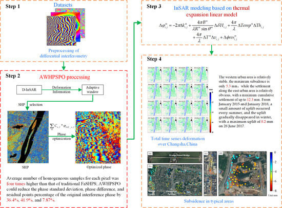
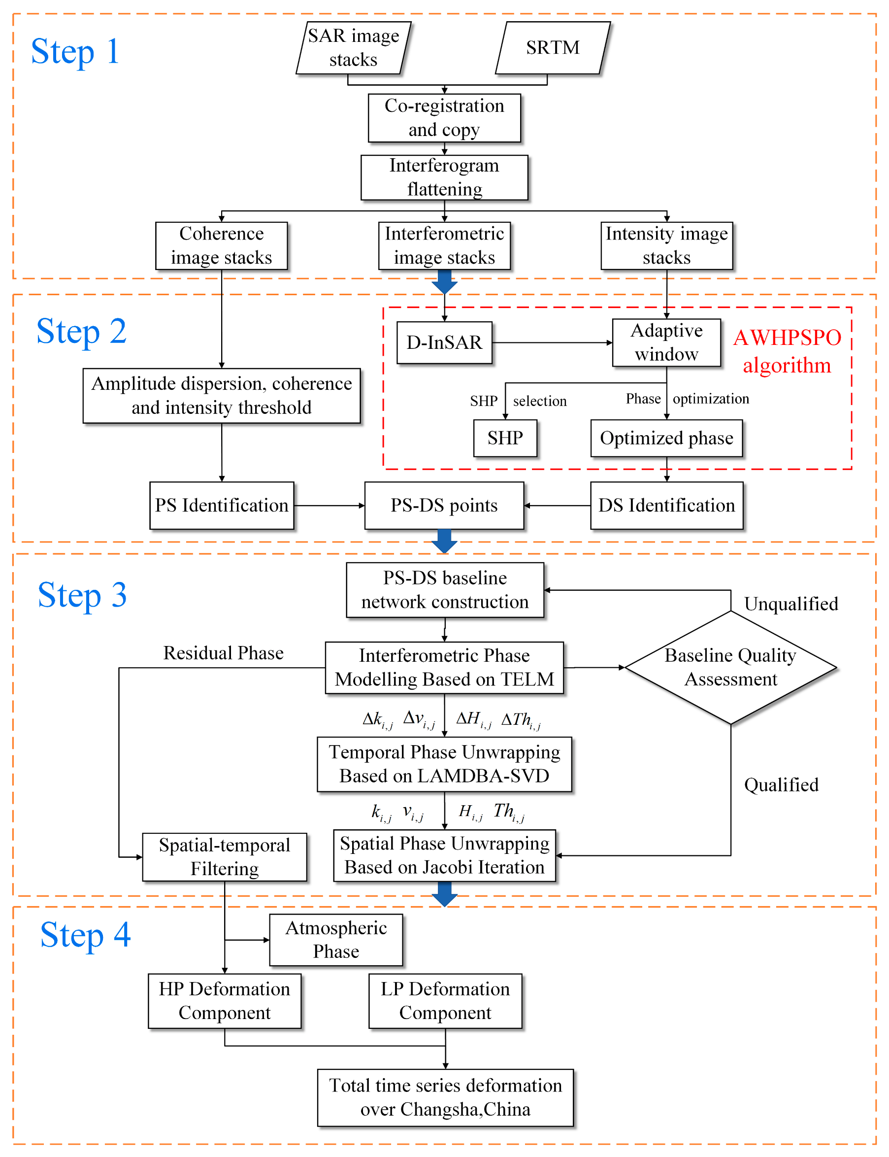
2.4. Processing Flow of the AWHPSPO Algorithm

The specific processing flow of AWHPSPO proposed in this paper is shown in Figure 1, and the main steps are as follows:

(1) Differential interferometric preprocessing, including coregistration, interferogram flattening, and topographic phase removal with external shuttle radar topography mission (SRTM), digital elevation model (DEM), etc. The corresponding coherence images, intensity images, and wrapped interferometric images are generated.

(2) PS-DS candidate identification considering deformation information. Firstly, SHP selection with an adaptive window considering the deformation information is carried out to extract PS and DS candidate points; then, phase optimization with an adaptive window considering the deformation information is implemented.

(3) PS-DS network construction, deformation modeling, and parameter estimation. Firstly, PS-DS network construction based on the Delaunay criterion over the extracted PS and DS candidate points is carried out; then, deformation modeling based on the thermal expansion linear model (TELM) is conducted; and finally, spatiotemporal unwrapping based on LAMDBA-SVD and the Jacobi iteration for the whole PS-DS network is implemented.

(4) Total time-series deformation generation. Firstly, the spatial and temporal filtering of the residual phase is performed to extract the residual high-pass deformation components; then, high-pass deformation components are superimposed with the low-pass deformation components to obtain the total time-series deformation over Changsha, China.

3. Experiment

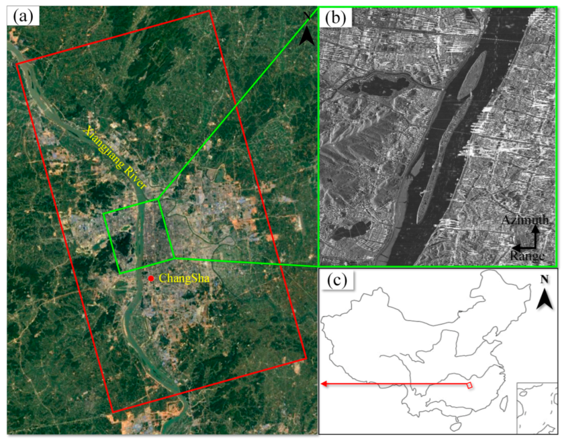
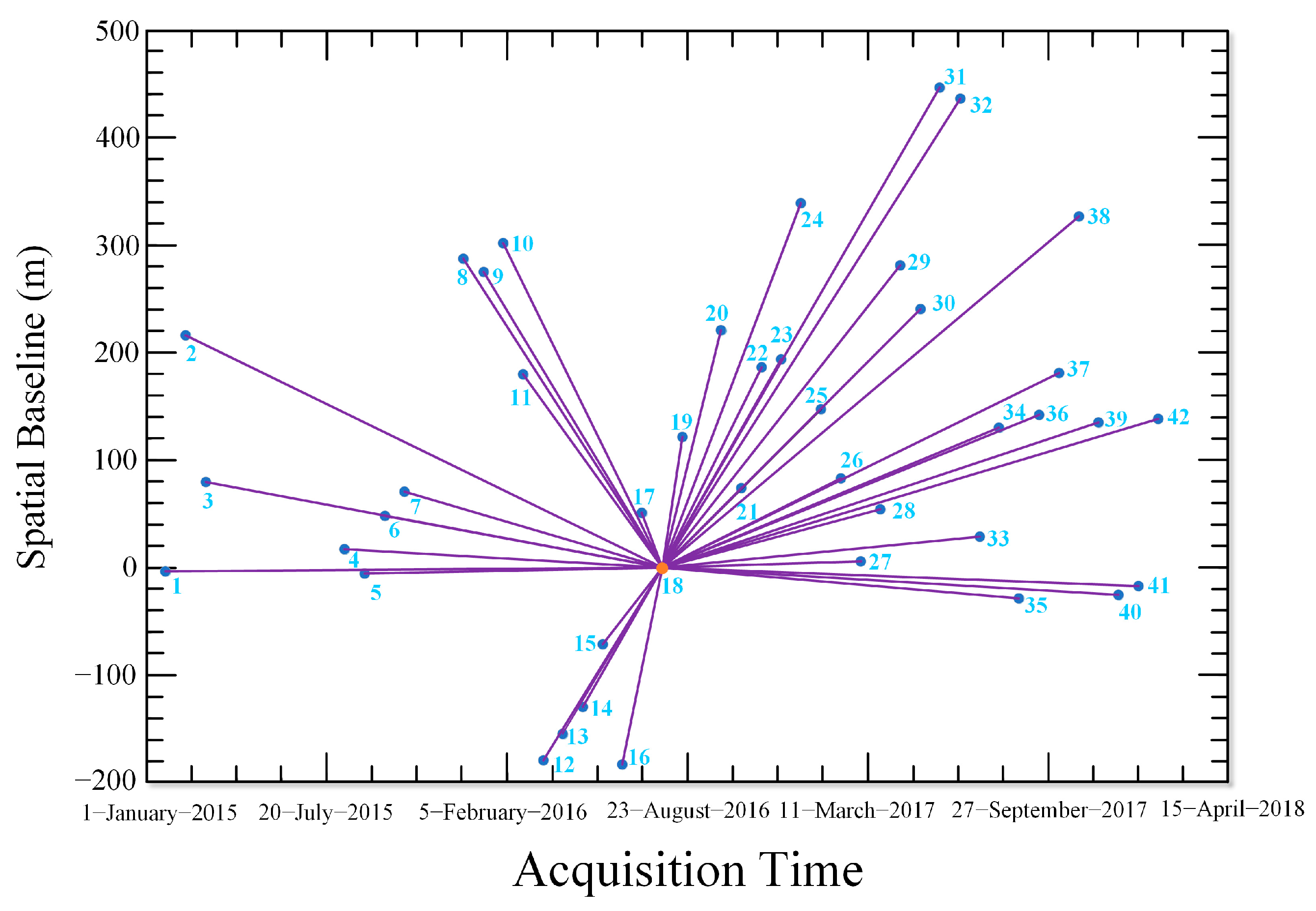
3.1. Background of the Study Area and Interferometry Preprocessing

Changsha is located in the northeastern part of Hunan Province, China, and is an important central city in the middle reaches of the Yangtze River. Orange Island, located in the center of Changsha, is an alluvial island formed by the sediment deposition action of the flowing water. The Orange Bridge is a hyperbolic arch bridge connecting Yuelu District and Furong District, crossing Xiang River and Orange Island. Sandy soil is the main soil component in this area. As a densely populated city with a population of 10 million, plenty of residential areas and well-developed infrastructures are distributed in this area. The long-term rapid urban construction has induced accumulated slow deformations over the surrounding infrastructures. Every flood season, the residential areas around Xiang River are under great potential danger of accumulated deformation, the collapse of the ground surface, or even landslides of the slope, which greatly endangers the safety of the area. Consequently, it is important to implement long-term spatiotemporal subsidence monitoring over the area, which can assist in understanding the health status of the area and potentially be used in traffic safety prevention. As shown in Figure 2, the red rectangle represents the spatial coverage of TerraSAR-X images used in the experiment, and the green subrectangle is the interesting subarea covering Orange Island.

A total of 42 TerraSAR-X stripmap (3 m × 3 m) satellite images with an average incidence angle of approximately 37.28° and a sampling interval of 22 days from January 2015 to January 2018 were collected for the experiment. The differential interferometry was carried out using the GAMMA MSP (modular SAR processor) processing module, and 30 m-resolution SRTM DEM (shuttle radar topography mission digital elevation model) data were used to remove the topographic phase. In order to ensure the original resolution of the image, the multilook ratio was set as 1:1. A single master image interferometric processing flow of PSI technology was utilized for the total data processing, with the image acquired on 24 August 2016 as the master image. The spatiotemporal baselines are shown in Figure 3. A total of 41 interferograms were generated after the processing of flat earth phase removal, filtering, the topographic phase, and orbit refinement.

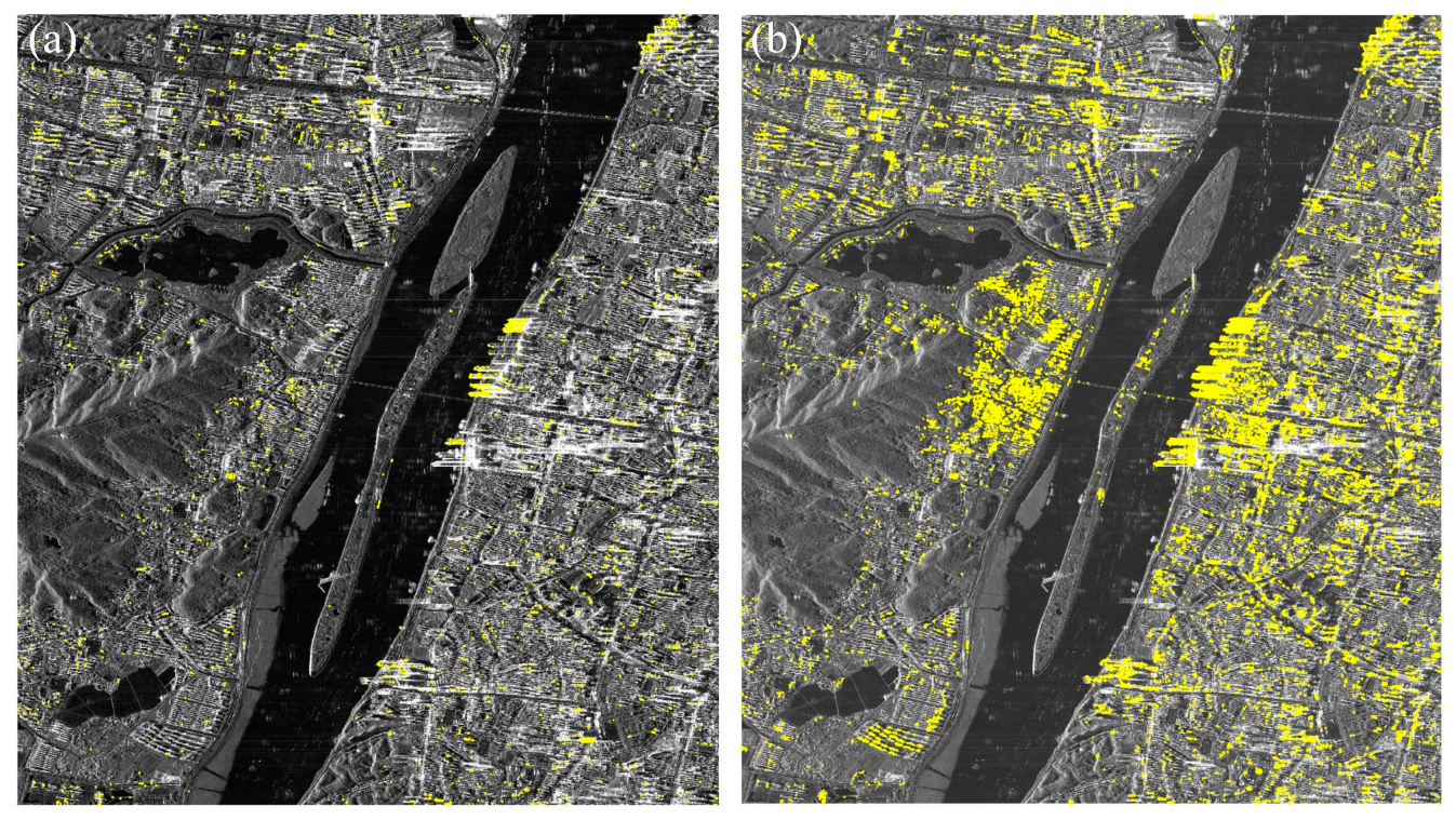
3.2. PS-DS SHP Selection

As introduced in Section 2.1, firstly, the window size for SHP identification was determined using the information on the deformation phases generated by the D-InSAR process with the first and last image of the SAR stacks. To ensure sufficient samples of SHP, the upper and lower thresholds of the SHP window were set as [15, 15] and [7, 7], respectively. Thus, the window size for each SHP was calculated by the adaptive window SHP identification method pixel by pixel on the image, considering the surrounding deformation phase information within the window. The number of SHPs over each pixel was calculated via the FaSHPS method.

Table 1. Comparison of the number of SHPs (statistically homogeneous points).

Average SHP Number Interval for a Pixel	Total Pixel Number of an Image via FaSHPS	Total Pixel Number of an Image via AWHPSPO
10 ≤ SHP < 20 *	1.37 × 107	1.43 × 107
20 ≤ SHP < 30	9.45 × 106	1.08 × 107
30 ≤ SHP < 40	5.76 × 106	7.49 × 106
40 ≤ SHP < 225	3.31 × 106	5.01 × 106
Average number of detected SHPs around a pixel	13	17

* When 10 ≤ SHPs < 20, this represents 10 to 20 SHPs being detected in the window centered on that pixel. The last row represents the average number of detected SHPs around each pixel for different methods.

shows the comparison of the total number of SHPs over the image and the average numbers around each pixel generated by the two methods. The window size for FaSHPS was set as [7, 7]. It can be seen that the average number of homogeneous samples for each pixel was four times higher than that of traditional FaSHPS, and the numbers of SHP within different intervals were all improved, with a maximum improvement of 51.6%. Figure 4 illustrates the comparison of the spatial distribution of SHP identification. From this figure, we can see that the distribution of homogeneous samples is lower in urban areas and higher in mountainous areas, comparatively. Take areas A and C in Figure 4c, for instance; the two areas belong to vegetated and bare land areas, with a total number of SHPs of approximately 5.7 × 10⁶ pixels when the average SHP number interval for a pixel is higher than 20; in contrast, area B is located in the high-rise group of Wanda Plaza, with densely distributed strong scatters of PS targets. The SHP number in this area is only approximately 1.3 × 10⁶ when the average SHP number interval for a pixel is lower than 10.

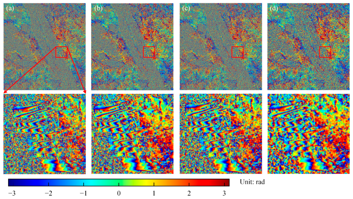
3.3. Phase Optimization

Three algorithms of phase optimization, Goldstein phase optimization, Gaussian-weighted phase optimization, and adaptive window phase optimization, were carried out as part of a comparative experiment. Goldstein filtering is the most commonly used filtering method for interferometric phases, whereas Gaussian-weighted filtering is the current phase optimization method used by mainstream software, including GAMMA software. The original differential interferogram (interferometric pair of 11 July 2016 and 8 February 2016) was selected. The comparison results before and after phase optimization are shown in Figure 5. It can be seen that the original differential interferogram has a great degree of speckle noise induced by temporal decorrelation, which hides the real deformation fringes. After phase optimization, optimized phases were improved, and the details of interference fringes were enhanced. After using the adaptive window phase optimization, the filtering quality of the interferogram was significantly improved, and the details of the interference fringes were more integrated compared with the original interference phase map.

To quantitively evaluate the quality of the optimized phases, three evaluation indicators—phase standard deviation, phase gradient, and residual phase ratio—were used here; the corresponding comparison results are shown in

Table 2. Quality evaluation of differential interferograms.

	Indicator	Phase Standard Deviation		Sum of Phase Differences		Percentage of RPs
Method		Average Value/Rad	Improvement	Average Value/Rad	Improvement
Original Interferogram		1.32	-	1.48	-	12.18%
Goldstein		1.11	15.9%	1.22	17.6%	7.94%
Gaussian-weighted		1.04	21.2%	1.16	21.6%	6.46%
Adaptive Window		0.84	36.4%	0.86	41.9%	4.31%

. The values of the phase standard deviation and the sum of phase differences can reflect the phase smoothness. The lower the phase standard deviation, the smoother the phase, and the higher the interferometric phase quality. Residual points (RP) represent the points where the integration values of four adjacent pixels’ interferogram gradients are nonzero along a certain direction. A too-high percentage of RPs will significantly affect the stability and reliability of the optimized fringes, so the percentage of RP is an important indicator.

As shown in Table 2, Goldstein filtering can reduce the phase standard deviation, phase difference, and RP percentage of the original interference phase by 15.9%, 17.6%, and 4.24%, respectively. Gaussian-weighted filtering can reduce the phase standard deviation, phase difference, and RP percentage of the original interference phase by 21.2%, 21.6%, and 6.46%, respectively. In contrast, the improvements in the results of our proposed algorithm were 36.4%, 41.9%, and 7.87%, respectively, with the phase noise being suppressed to a larger extent. This indicates that the decorrelation noise can be effectively suppressed by the adaptive window, and the phases can be smoother and more continuous in spatial distribution, which will be used in the following PS-DS identification. The adaptive window considering the deformation phase information was used for SHP selection and phase optimization in the subsequent experiments. The distributed targets with better coherence, a higher signal-to-noise ratio, and high-quality, optimized phase information can be selected as PS or DS candidates in the subsequent processing.

After the SHP identification and phase optimization, a pixel with a coherence value higher than 0.5 and an SHP number higher than 30 is considered a DS candidate. PS candidates were extracted by the triple index threshold considering the amplitude deviation threshold, coherence, and intensity, with the corresponding thresholds set as 0.32, 0.9, and 6, respectively [34,35,36]. In total, 5299 PS candidates were extracted, which is shown in Figure 6a. The final extracted DS candidates are shown in Figure 6b. It can be seen from the figure that the extracted DS points greatly improve the density of high-coherence points in the region, which can better compensate for the low spatial density of sparse PS targets.

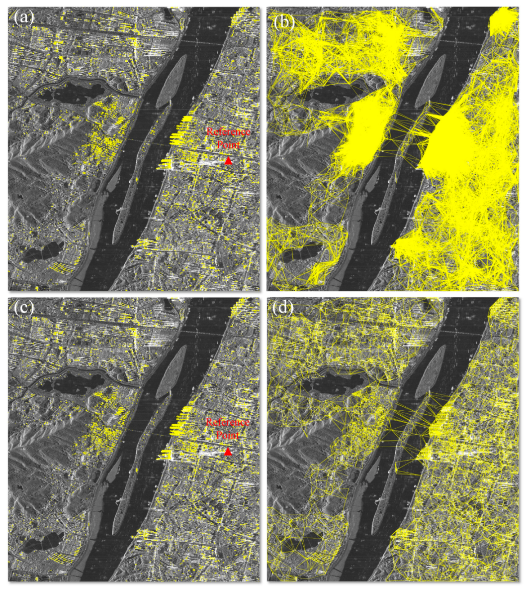
3.4. PS-DS Network Construction and Baseline Quality Assessment

The PS-DS baseline network is constructed based on a hierarchical network strategy. Firstly, the extracted PS targets are connected to construct a primary network using the Delaunay function. Then, the surrounding DS points, within the distance threshold of 300 m, are connected to the nearest PS in the primary network as a secondary network. Additionally, the phase model given in Equation (2) is established for each edge. In order to evaluate the quality of the baseline parameter valuation, the temporal correlation coefficients (TCC) of each baseline are calculated as the quality indicators [37], which can be written as

$${\gamma }_{base}=\frac{1}{n}{\displaystyle {\mathsf{\sum }}_{i=1}^n(\cos (\mathsf{\Delta }re{s}_{i,j}^m)+j\sin (\mathsf{\Delta }re{s}_{i,j}^m))}$$

(3)

where $\mathsf{\Delta }re{s}_{i,j}^m$ is the residual phase component, which can be obtained by substituting the estimated incremental values of the parameter. A threshold value for ${\gamma }_{base}$ is set to eliminate the low-quality edges (including isolated PS and DS candidates), and then the network is rearranged. This is an iterative process until all baselines satisfy the threshold value. Finally, a total of 33,198 PS and DS points and 44,262 baselines were extracted over the study area. The final constructed PS-DS baseline network is shown in Figure 7.

4. Results

4.1. Model Parameter Estimation Results

Figure 8 shows the estimated average subsiding velocities and thermal expansion parameters over the area, and Figure 8b shows a plot of the thermal expansion coefficient. From the spatial distribution, most of the region is stable, with the color varying from yellow to green, and the annual deformation rates fall mainly within [−2, 2] mm/y. There still exist scattered uplift points in the area, which we suggest are related to the residual atmospheric delay errors and gross error points wrongly identified as PS or DS targets. Four typical subsiding areas (areas D, E, F, and I) are presented in Figure 8. Area D is the Orange Island Bridge, which connects Yuelu District and Furong District, with a maximum sedimentation rate of −1.1 mm/y. Area E is located in the central area of the eastern Xiangjiang River, with a maximum sedimentation rate of −1.5 mm/y, while area F is near International Finance Square building, with a maximum sedimentation rate of −1.8 mm/y. Area I is located in Poly International Plaza, with a maximum sedimentation rate of −1.7 mm/y.

Figure 8b shows the obtained thermal expansion coefficients of all targets over the area. Statistically, the thermal expansion coefficients of 85% of the PS-DS targets are within the range of [−0.05, 0.05], and 99% are within [−0.1, 0.1]. Due to the complex infrastructures with different heights in the Orange District, there existed significant differences in the values of the coefficient of the thermal expansion coefficients. According to Monserrat [38], the parameters of the thermal expansion characteristics are considered equivalent when different infrastructures are made of similar materials, and the value of the thermal expansion coefficient is proportional to the height of the building. The distribution of thermal expansion coefficients in area D and area G (Figure 8c,d) also proves this. The Orange Island Bridge in area D and the outpatient building of Xiangya No. 1 Hospital in area G are examples of typical urban infrastructures, and the thermal expansion characteristic parameter of the material can be estimated using the following equation, which is expressed as

$$K=\frac{\mathrm{T}h}{H}$$

(4)

where $K$ and $\mathrm{T}h$ define the thermal expansion characteristic parameter and thermal expansion coefficient mentioned in Section 2.3, respectively. $H$ denotes the height of the infrastructures. According to our estimations, the average thermal expansion characteristic parameter of the bridge material in area D is 9.5 × 10⁻⁶/°C, and 7.4 × 10⁻⁶/°C for the outpatient building of Xiangya No. 1 Hospital in area G. According to our in situ investigation, the material of Orange Island Bridge is No. 200 concrete, and the outpatient building of Xiangya No. 1 Hospital is ordinary No. 32.5 concrete. The magnitude of thermal expansion characteristic parameters for these two kinds of concrete that are poured with different material ratios was approximately within the range of [6 × 10⁻⁶/°C,13 × 10⁻⁶/°C] [39,40]. The estimated results are consistent with the physical properties of the materials, which proves the reliability of the proposed method.

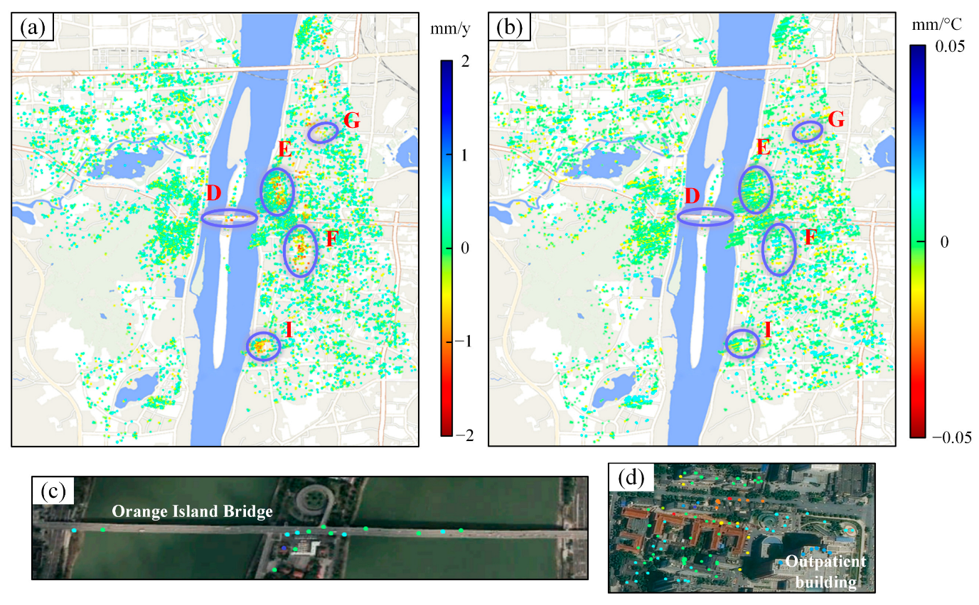
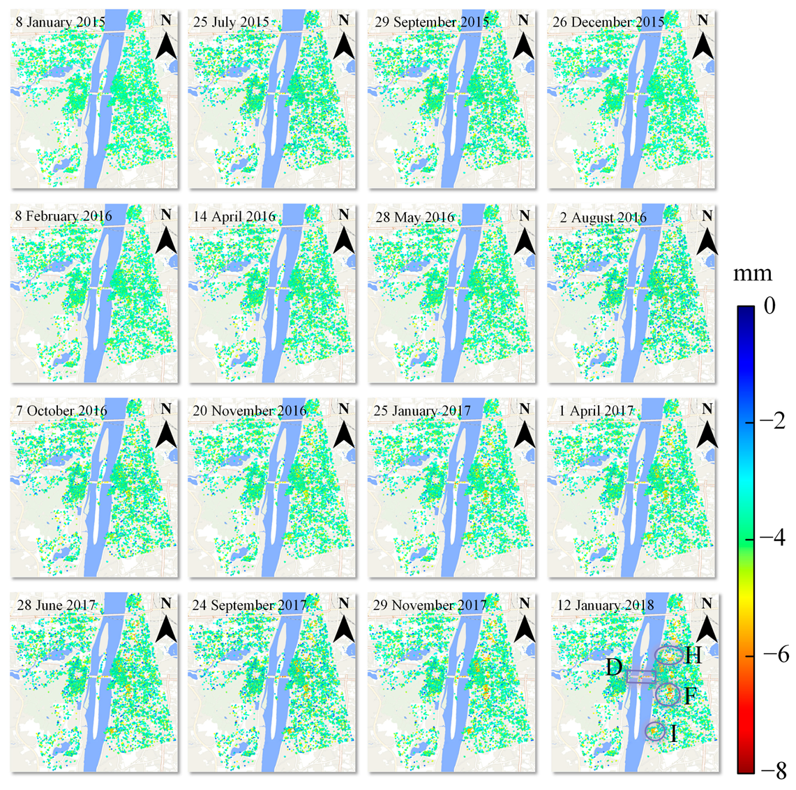
4.2. Time-Series Deformation Estimation Results

Figure 9 shows three years of cumulative time-series deformation results from the study area obtained by the AWHPSPO algorithm. From the spatial distribution, among the stable varying characteristics in the area, the settlement along the east bank of Xiangjiang River is relatively obvious, with a maximum cumulative settlement of up to 12.3 mm. Area F (near International Finance Square building in Changsha), Area H (near Zhongshan Pavilion), and area I (near Poly International Plaza) on the east bank of Xiangjiang River are extracted as typical subsiding areas, and their specific locations are shown in the last picture of Figure 9. The corresponding enlarged images for these areas are shown in Figure 10.

The maximum settlement in area D is located near the center of the bridge, while area H is located near Zhongshan Pavilion; area F is near the International Finance Square building, and area I is near Poly International Plaza. The quantitative maximum cumulative settlements are shown in

Table 3. Accumulated subsidence in typical areas.

Region	Accumulated Subsidence (mm)
Area D (Orange Island Bridge area)	−5.5
Area F (area near International Finance Square)	−6.6
Area H (area near Zhongshan Pavilion)	−5.7
Area I (Poly International Plaza)	−5.8

.

Compared with the east bank of the Xiangjiang River, the western urban area of the Xiangjiang River is relatively stable, with a maximum cumulative subsidence of only 5.3 mm. From January 2015 and January 2018, a small amount of uplift occurred every summer, and the uplift gradually disappeared in winter, with a maximum uplift of 8.2 mm on 28 June 2017. By consulting the hydro-meteorological data of Changsha City, it can be seen that the large amount of rainfall in the rainy months increases the water content of the land and raises the groundwater level underground, thus leading to ground uplift, which will be discussed in Section 5.

Temporally, the area along the east bank of Xiangjiang River was relatively stable from 8 January 2015 to 11 July 2016, subsiding from 2 August 2016 to 12 January 2018, with a maximum settlement of 12.3 mm. When consulting the historical information of this area, it can be seen that a large amount of building demolition infrastructure work was carried out in areas G and I around 2017 (see Figure 11), and engineering construction was suggested as the main reason for the settlement here.

5. Analysis and Discussion

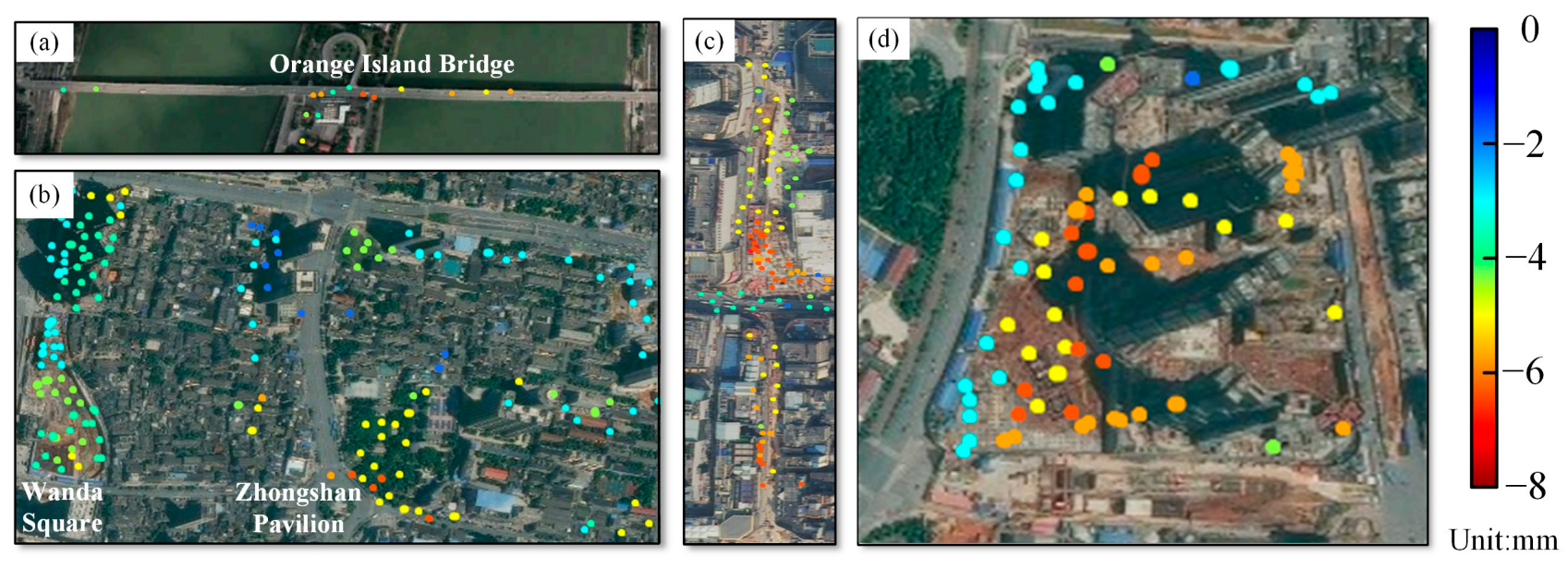
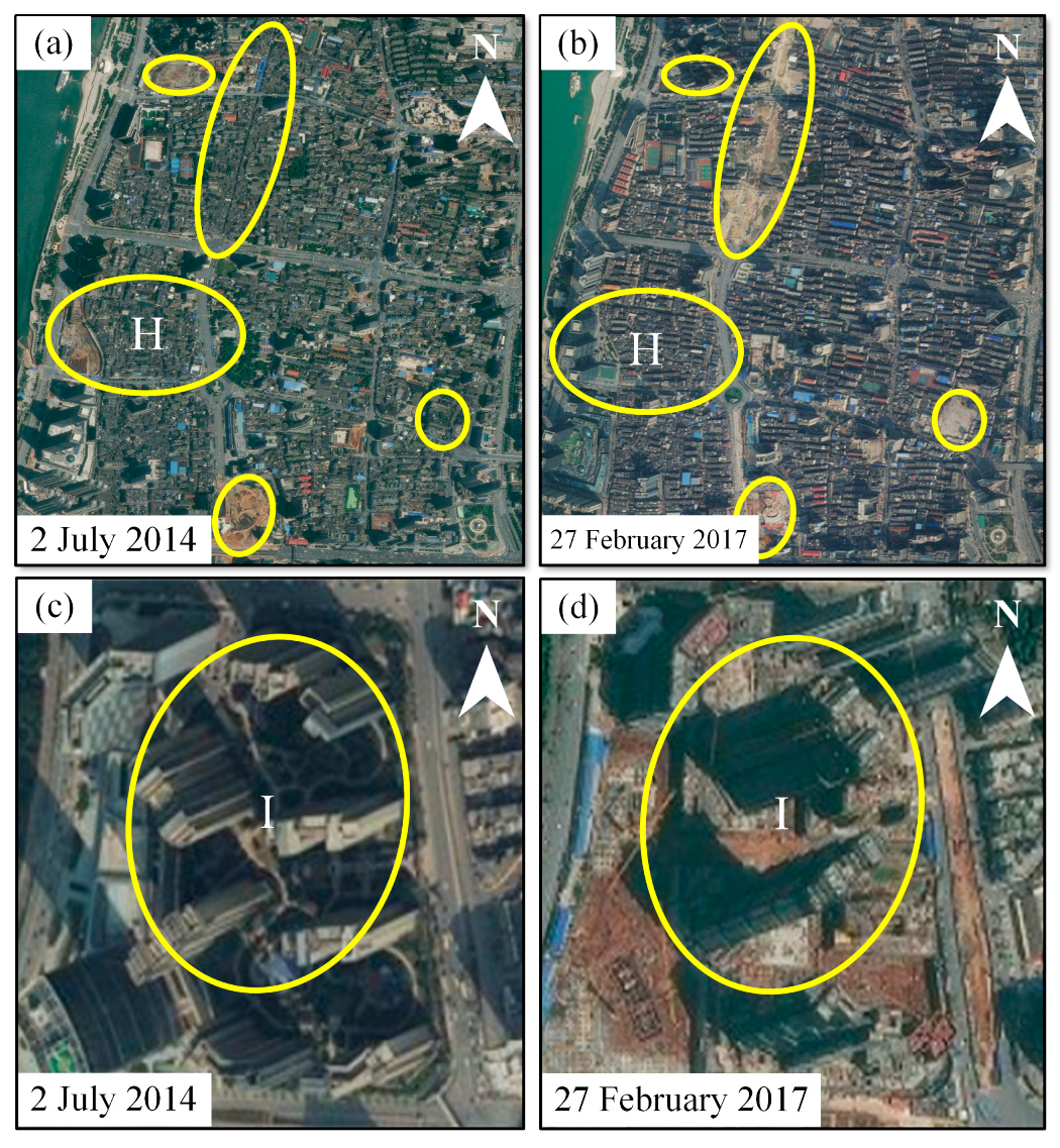
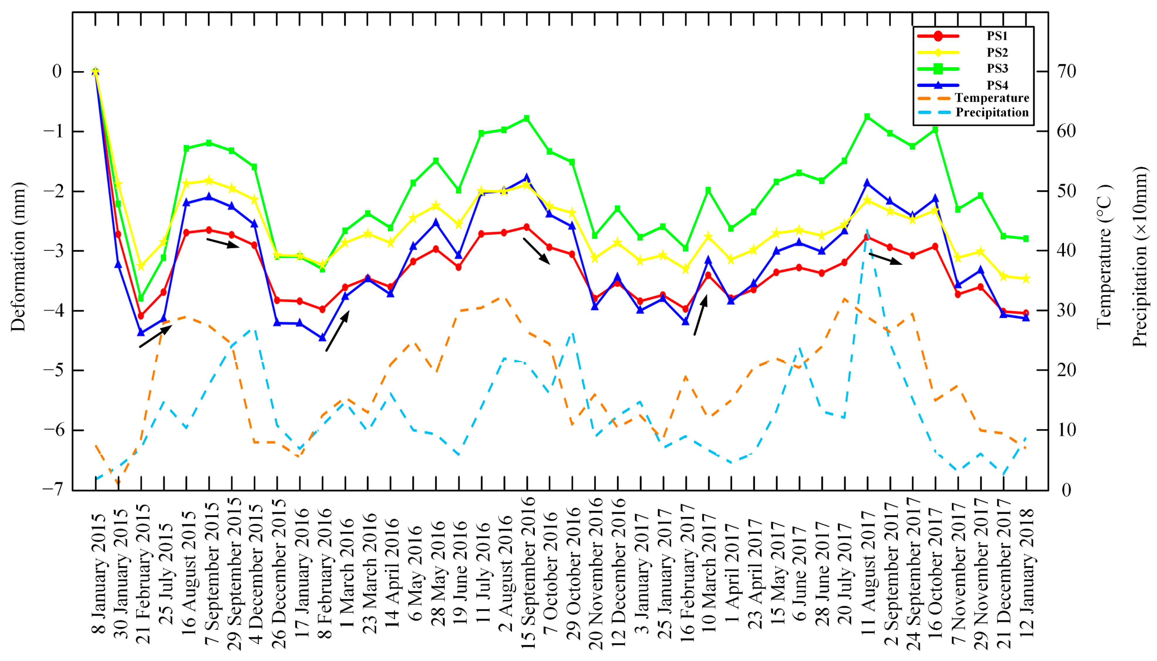
5.1. Analysis of Time-Series Deformation at Feature Points

In order to quantitatively show the temporal evolution of the deformation, four feature points were extracted, and their corresponding in situ locations are shown in Figure 12. The temperature data in Equation (2) were obtained using the average temperature of Changsha City from the China Meteorological Administration website [41]. As shown in Figure 12, both PS1 and PS2 are located on the bridge deck of the Orange Bridge, PS3 is located on the southeast corner of the roof of the Hunan Provincial Traffic Design Institute building, and PS4 is located on the west corner of the roof of the Changsha Christian Church City North Church. The three-year cumulative time-series deformations are shown in Figure 13. The maximum accumulated subsidence is 4.0 mm for PS1, 3.5 mm for PS2, 2.8 mm for PS3, and 4.1 mm for PS4. The maximum settlement at PS4, for example, occurred on 8 February 2016, reaching up to 4.5 mm. It can be seen from the figure that three uplifts (from 21 February 2015 to 16 August 2015, from 8 February 2016 to 15 September 2016, and from 16 February 2017 to 11 August 2017) with a magnitude within [2, 3] mm were detected.

In order to further reveal the subsiding characteristics of the infrastructures, the average external temperature and precipitation data for Changsha during the observation periods were collected. The subsidence is converted from the line-of-sight deformation to the vertical direction using the equation $S_v=\frac{S_{LOS}}{\cos \theta }$. The climate of Changsha is characterized by a monsoon climate with high temperatures and lots of rain in summer, cold and little rain in winter, and a high-temperature period coinciding with the rainy period. Since China is located in the eastern part of Asia and Europe (the world’s largest continent), on the west coast of the Pacific Ocean (the world’s largest ocean), and the southwest is close to the Indian Ocean, the climate is significantly influenced by the continent and the ocean. Winter winds are generated inland in Asia and are cold and dry, under the influence of which Changsha generally has low precipitation and low temperatures in winter. Summer winds come from the Pacific Ocean in the southeast and the Indian Ocean in the southwest, which is warm and humid, and under its influence, precipitation generally increases, resulting in rain and heat during the same period. From the figure, it can be seen that there existed strong correlations between the vertical deformation curve and both temperature and precipitation. When considering the external air temperature data, it can be seen that the thermal expansion effect causes vertical upward displacement during the summer months (July to September) every year, which is related to a rising temperature, while vertical downward displacements are related to the dropping temperature from September to November. Through the collected hydro-meteorological data, it was found that the annual rainfall in Changsha increases significantly in warm seasons (February to September) and decreases in cold seasons (October to January). It is assumed that the large amount of rainfall during the rainy season increases the water content underground and raises the groundwater level in some areas, thus leading to ground uplift. Among the four feature points, PS1 and PS2 are located on the bridge deck of the Orange Bridge, and the settlement difference between summer and winter is approximately 1.3 mm, which is more stable than that of PS3 and PS4. In contrast, PS3 and PS4, located on the top of the building, are more susceptible to thermal expansion effects, leading to fluctuations in displacement along the vertical direction. According to our correlation analysis, the correlation coefficients between the vertical deformations and temperature for the four feature points were estimated as 0.89, 0.84, 0.86, and 0.88, respectively.

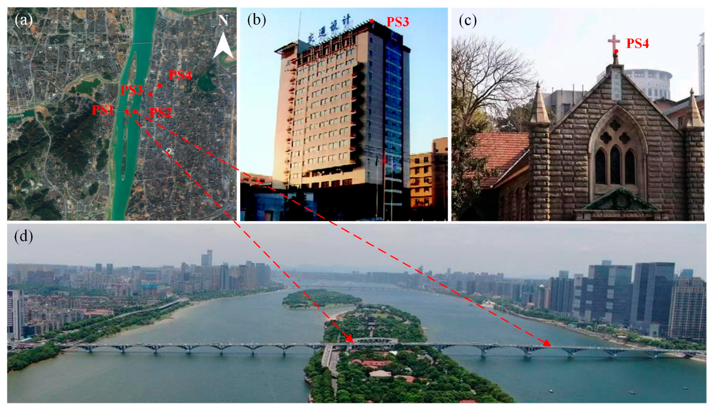
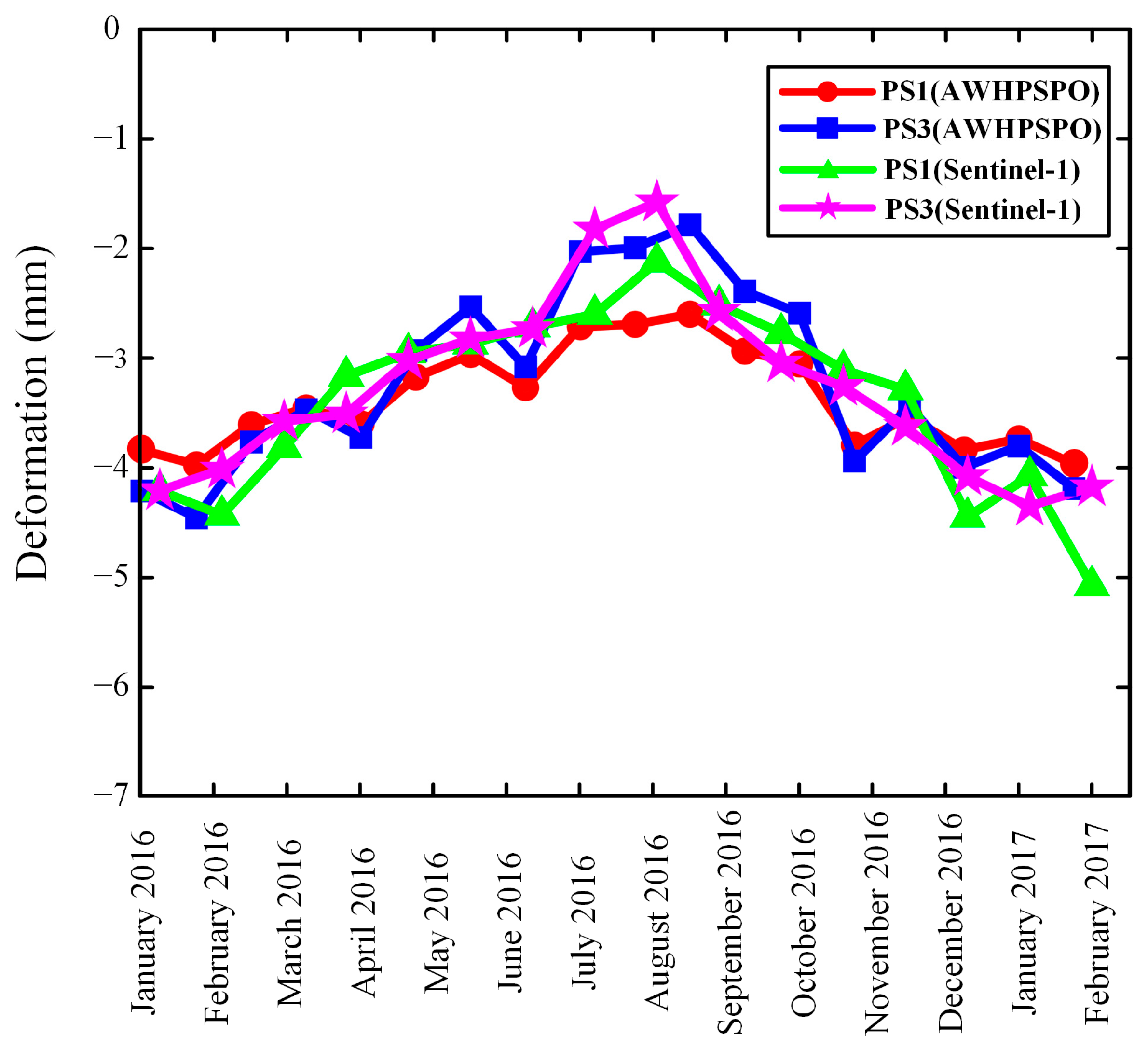
5.2. Accuracy Analysis

In order to compensate for the lack of external in situ deformation measurements, the external accuracy of the experimental results can be assessed using a crossvalidation method when no external field-level data are available [42]. In total, 16 Sentinel-1A SAR images from January 2016 to February 2017 were collected and processed using a traditional small baseline subset interferometric synthetic aperture radar (SBAS-InSAR) processing flow for crossvalidation. Two feature points were extracted for the crossvalidation comparison with the AWHPSPO results during the same temporal period in Figure 14.

By using the data solution method as the influencing factor, a one-way ANOVA (analysis of variance) was conducted on the deformation results of the two groups. ANOVA is a statistical test that is used to test the consistency of the means of two or more of the groups of samples. First, the root mean squares of the intergroup and between-group comparisons are calculated to generate the F distribution. Then, the critical values of the numerator and denominator degrees of freedom are extracted from the F distribution table, according to the given significance level α, which can be used to determine whether or not to accept the original hypothesis.

The results of the crossvalidation are shown in Figure 14 and

Table 4. Results of one-way ANOVA.

Statistical Items	PS1				PS3
	SS (Sum of Squares)	df (Degrees of Freedom)	MS (Root Mean Square)	F-Statistic	SS (Sum of Squares)	df (Degrees of Freedom)	MS (Root Mean Square)	F-Statistic
Between groups	0.0001	1	0.00012	0.00026	0.0001	1	0.0001	0.00015
Intergroup	13.7784	34	0.45928	-	20.5425	34	0.68475	-

. It can be seen from them that the two groups of deformation time-series results at the feature points derived by the two methods show high consistency. The root mean squares of the differences in PS1 and PS2 are estimated as 1.2 × 10⁻⁴ mm and 1 × 10⁻⁴ mm, and the F-values are 2.6 × 10⁻⁴ and 1.5 × 10⁻⁴, respectively. By looking up the F function distribution table, it can be concluded that under the condition of a 99% confidence interval, there is no significant difference between the two groups of results, which proves the accuracy of our proposed method. There has been one previous article on the monitoring of the deformation of Changsha city using SBAS-InSAR during 2017–2020, and the deformation magnitude is consistent with the results obtained in this study [43].

5.3. Discussion of AWHPSPO

(1) The main advantages of our proposed SHP identification and phase optimization algorithms are as follows: Firstly, the SHP window size can be flexibly adjusted according to the deformation information, which can improve the homogeneous samples of the experimental area. The average number of SHPs around the pixel is improved by four times that of traditional FaSHPS. Secondly, more smooth phases can be generated with adaptive window phase optimization considering the deformation information; thus, the accuracy of the subsequent deformation estimation can be further improved. The phase standard deviation and phase gradient were improved by 36.4% and 41.9%, respectively. Consequently, the new method can also compensate for the defects of insufficient homogeneous samples and low phase quality in traditional DS-InSAR processing.

(2) The experimental results show that the deformation in Orange Island is characterized temporally by slow subsiding variations and spatially by relatively high subsidence on the east bank of Xiangjiang River. By controlling the length of each baseline and the iterative evaluation of the temporal correlation coefficients for the whole PS-DS network, the error can be effectively controlled. According to the results, a subcentimeter-level magnitude of uplift can be accurately detected, indicating that our method is applicable for the long-term monitoring of slow urban deformation. Furthermore, by introducing the thermal expansion parameters into the InSAR deformation modeling, the thermal expansion coefficients can be estimated simultaneously with the deformation parameters, which can provide a reference for the related fields.

(3) Since there are no available external leveling measurements over the study area, SBAS-InSAR processing was used for crossvalidation to verify the accuracy of our proposed algorithm. The results indicate that under the condition of a 99% confidence interval, no significant difference between the two groups can be found, thus proving the accuracy. It would be more convincing if the analysis could be repeated with sufficient available external leveling measurements.

6. Conclusions

A novel time-series InSAR processing algorithm based on the AWHPSPO algorithm is proposed and applied for the monitoring of the slow deformation of urban areas. The algorithm improves the traditional DSI in three steps: SHP selection, phase optimization, and time-series InSAR deformation modeling. During the SHP selection and phase optimization steps, both the time-series intensity information and the deformation phase are considered, which can compensate for the defects of insufficient homogeneous samples and low phase quality in traditional DS-InSAR processing. During InSAR deformation modeling, the thermal expansion component is introduced into the traditional linear model, which considers the physical characteristics of the thermal expansion effect of the urban infrastructures, and the thermal expansion coefficients can be estimated simultaneously with the deformation parameters.

A total of 42 TerraSAR-X radar satellite images covering the Orange Island area in Changsha City, China, were collected in our experiment. The experimental results show that the 3 years of data for historical time-series deformation in this area are characterized by slow settlement, with a maximum settlement of 12.3 mm. The spatial distribution is characterized by relatively high subsidence on the east bank of Xiangjiang River, with the rest of the area being relatively stable. The thermal expansion parameters were generally distributed between −0.1 mm/°C and 0.1 mm/°C. The thermal expansion characteristic parameter of Orange Bridge and the Xiangya First Hospital building was estimated as 9.5 × 10⁻⁶/°C, 7.4 × 10⁻⁶/°C, which coincided with the characteristics of the main material.

In order to compensate for the lack of external in situ geodetic measurements, a crossvalidation with SBAS-InSAR results using the Sentinel 1A dataset was carried out to verify the accuracy of the obtained deformation time series. The root mean squares of the group differences between the two tested feature points were estimated as 1.2 × 10⁻⁴ mm and 1 × 10⁻⁴ mm, respectively, with no significant difference between the two monitoring results at a 99% confidence interval, which proves that the results obtained in this study are reliable.

References

1. Zhang, X.; Zhu, C.; He, M.; Dong, M.; Zhang, G.; Zhang, F. Failure Mechanism and Long Short-Term Memory Neural Network Model for Landslide Risk Prediction. Remote Sens. 2021, 14, 166. [Google Scholar] [CrossRef]
2. Song, S.; Zhao, M.; Zhu, C.; Wang, F.; Cao, C.; Li, H.; Ma, M. Identification of the Potential Critical Slip Surface for Fractured Rock Slope Using the Floyd Algorithm. Remote Sens. 2022, 14, 1284. [Google Scholar] [CrossRef]
3. Hooper, A.; Segall, P.; Zebker, H. Persistent Scatterer Interferometric Synthetic Aperture Radar for Crustal Deformation Analysis, with Application to Volcán Alcedo, Galápagos. J. Geophys. Res. 2007, 112, B07407. [Google Scholar] [CrossRef] [Green Version]
4. Zhang, S.; Si, J.; Niu, Y.; Zhu, W.; Fan, Q.; Hu, X.; Zhang, C.; An, P.; Ren, Z.; Li, Z. Surface Deformation of Expansive Soil at Ankang Airport, China, Revealed by InSAR Observations. Remote Sens. 2022, 14, 2217. [Google Scholar] [CrossRef]
5. Crosetto, M.; Monserrat, O.; Cuevas-González, M.; Devanthéry, N.; Crippa, B. Persistent Scatterer Interferometry: A Review. ISPRS J. Photogramm. Remote Sens. 2016, 115, 78–89. [Google Scholar] [CrossRef] [Green Version]
6. Shen, C.; Feng, Z.; Xie, C.; Fang, H.; Zhao, B.; Ou, W.; Zhu, Y.; Wang, K.; Li, H.; Bai, H.; et al. Refinement of Landslide Susceptibility Map Using Persistent Scatterer Interferometry in Areas of Intense Mining Activities in the Karst Region of Southwest China. Remote Sens. 2019, 11, 2821. [Google Scholar] [CrossRef] [Green Version]
7. Ma, P.; Li, T.; Fang, C.; Lin, H. A Tentative Test for Measuring the Sub-Millimeter Settlement and Uplift of a High-Speed Railway Bridge Using COSMO-SkyMed Images. ISPRS J. Photogramm. Remote Sens. 2019, 155, 1–12. [Google Scholar] [CrossRef]
8. Zhu, M.; Wan, X.; Fei, B.; Qiao, Z.; Ge, C.; Minati, F.; Vecchioli, F.; Li, J.; Costantini, M. Detection of Building and Infrastructure Instabilities by Automatic Spatiotemporal Analysis of Satellite SAR Interferometry Measurements. Remote Sens. 2018, 10, 1816. [Google Scholar] [CrossRef] [Green Version]
9. Dittrich, J.; Hölbling, D.; Tiede, D.; Sæmundsson, Þ. Inferring 2D Local Surface-Deformation Velocities Based on PSI Analysis of Sentinel-1 Data: A Case Study of Öræfajökull, Iceland. Remote Sens. 2022, 14, 3166. [Google Scholar] [CrossRef]
10. Li, G.; Ding, Z.; Li, M.; Hu, Z.; Jia, X.; Li, H.; Zeng, T. Bayesian Estimation of Land Deformation Combining Persistent and Distributed Scatterers. Remote Sens. 2022, 14, 3471. [Google Scholar] [CrossRef]
11. Jiang, M.; Yong, B.; Tian, X.; Malhotra, R.; Hu, R.; Li, Z.; Yu, Z.; Zhang, X. The Potential of More Accurate InSAR Covariance Matrix Estimation for Land Cover Mapping. ISPRS J. Photogramm. Remote Sens. 2017, 126, 120–128. [Google Scholar] [CrossRef]
12. Jänichen, J.; Schmullius, C.; Baade, J.; Last, K.; Bettzieche, V.; Dubois, C. Monitoring of Radial Deformations of a Gravity Dam Using Sentinel-1 Persistent Scatterer Interferometry. Remote Sens. 2022, 14, 1112. [Google Scholar] [CrossRef]
13. Li, Y.; Zuo, X.; Zhu, D.; Wu, W.; Yang, X.; Guo, S.; Shi, C.; Huang, C.; Li, F.; Liu, X. Identification and Analysis of Landslides in the Ahai Reservoir Area of the Jinsha River Basin Using a Combination of DS-InSAR, Optical Images, and Field Surveys. Remote Sens. 2022, 14, 6274. [Google Scholar] [CrossRef]
14. Liu, Y.; Ma, P.; Lin, H.; Wang, W.; Shi, G. Distributed Scatterer InSAR Reveals Surface Motion of the Ancient Chaoshan Residence Cluster in the Lianjiang Plain, China. Remote Sens. 2019, 11, 166. [Google Scholar] [CrossRef]
15. Ferretti, A.; Fumagalli, A.; Novali, F.; Prati, C.; Rocca, F.; Rucci, A. A New Algorithm for Processing Interferometric Data-Stacks: SqueeSAR. IEEE Trans. Geosci. Remote Sens. 2011, 49, 3460–3470. [Google Scholar] [CrossRef]
16. Fornaro, G.; Verde, S.; Reale, D.; Pauciullo, A. CAESAR: An Approach Based on Covariance Matrix Decomposition to Improve Multibaseline–Multitemporal Interferometric SAR Processing. IEEE Trans. Geosci. Remote Sens. 2015, 53, 2050–2065. [Google Scholar] [CrossRef]
17. Jiang, M.; Guarnieri, A.M. Distributed Scatterer Interferometry with the Refinement of Spatiotemporal Coherence. IEEE Trans. Geosci. Remote Sens. 2020, 58, 3977–3987. [Google Scholar] [CrossRef]
18. Shi, G.; Ma, P.; Lin, H.; Huang, B.; Zhang, B.; Liu, Y. Potential of Using Phase Correlation in Distributed Scatterer InSAR Applied to Built Scenarios. Remote Sens. 2020, 12, 686. [Google Scholar] [CrossRef] [Green Version]
19. Even, M.; Schulz, K. InSAR Deformation Analysis with Distributed Scatterers: A Review Complemented by New Advances. Remote Sens. 2018, 10, 744. [Google Scholar] [CrossRef] [Green Version]
20. Sun, Q.; Jiang, L.; Jiang, M.; Lin, H.; Ma, P.; Wang, H. Monitoring Coastal Reclamation Subsidence in Hong Kong with Distributed Scatterer Interferometry. Remote Sens. 2018, 10, 1738. [Google Scholar] [CrossRef] [Green Version]
21. Li, G.; Zhao, C.; Wang, B.; Liu, X.; Chen, H. Land Subsidence Monitoring and Dynamic Prediction of Reclaimed Islands with Multi-Temporal InSAR Techniques in Xiamen and Zhangzhou Cities, China. Remote Sens. 2022, 14, 2930. [Google Scholar] [CrossRef]
22. Samiei-Esfahany, S.; Martins, J.E.; van Leijen, F.; Hanssen, R.F. Phase Estimation for Distributed Scatterers in InSAR Stacks Using Integer Least Squares Estimation. IEEE Trans. Geosci. Remote Sens. 2016, 54, 5671–5687. [Google Scholar] [CrossRef] [Green Version]
23. Jiang, M.; Miao, Z.; Gamba, P.; Yong, B. Application of Multitemporal InSAR Covariance and Information Fusion to Robust Road Extraction. IEEE Trans. Geosci. Remote Sens. 2017, 55, 3611–3622. [Google Scholar] [CrossRef]
24. Jiang, M.; Ding, X.; Hanssen, R.F.; Malhotra, R.; Chang, L. Fast Statistically Homogeneous Pixel Selection for Covariance Matrix Estimation for Multitemporal InSAR. IEEE Trans. Geosci. Remote Sens. 2015, 53, 1213–1224. [Google Scholar] [CrossRef]
25. Jiang, M.; Ding, X.; Tian, X.; Malhotra, R.; Kong, W. A Hybrid Method for Optimization of the Adaptive Goldstein Filter. ISPRS J. Photogramm. Remote Sens. 2014, 98, 29–43. [Google Scholar] [CrossRef]
26. Jiang, M.; Ding, X.; Li, Z. Hybrid Approach for Unbiased Coherence Estimation for Multitemporal InSAR. IEEE Trans. Geosci. Remote Sens. 2014, 52, 2459–2473. [Google Scholar] [CrossRef]
27. Dong, L.; Wang, C.; Tang, Y.; Zhang, H.; Xu, L. Improving CPT-InSAR Algorithm with Adaptive Coherent Distributed Pixels Selection. Remote Sens. 2021, 13, 4784. [Google Scholar] [CrossRef]
28. Li, S.; Zhang, S.; Li, T.; Gao, Y.; Zhou, X.; Chen, Q.; Zhang, X.; Yang, C. An Adaptive Weighted Phase Optimization Algorithm Based on the Sigmoid Model for Distributed Scatterers. Remote Sens. 2021, 13, 3253. [Google Scholar] [CrossRef]
29. Lin, K.-F.; Perissin, D. Identification of Statistically Homogeneous Pixels Based on One-Sample Test. Remote Sens. 2017, 9, 37. [Google Scholar] [CrossRef] [Green Version]
30. Wang, Y.; Deng, Y.; Fei, W.; Wang, R.; Song, H.; Wang, J.; Li, N. Modified Statistically Homogeneous Pixels’ Selection with Multitemporal SAR Images. IEEE Geosci. Remote Sens. Lett. 2016, 13, 1930–1934. [Google Scholar] [CrossRef]
31. Kampes, B.M.; Hanssen, R.F. Ambiguity Resolution for Permanent Scatterer Interferometry. IEEE Trans. Geosci. Remote Sens. 2004, 42, 2446–2453. [Google Scholar] [CrossRef] [Green Version]
32. Teunissen, P.J.G. The Least-Squares Ambiguity Decorrelation Adjustment: A Method for Fast GPS Integer Ambiguity Estimation. J. Geod. 1995, 70, 65–82. [Google Scholar] [CrossRef]
33. Jun, Z.; Lingjie, Z.; Xuemin, X.; Rui, Z.; Liang, B.; Tengfei, Z.; Haodan, B. Joint Estimation Method of Time-Series InSAR Deformation and Environmental Physical Parameters for Soft Clay Area over Dongting Lake. Available online: https://kns.cnki.net/kcms/detail/11.2089.P.20221019.1026.002.html (accessed on 11 December 2022). (In Chinese).
34. Qiang, C.; Xiaoli, D.; Guoxiang, L.; Jyrching, H.U.; Linguo, Y. Baseline recognition and parameter estimation of persistent-scatterer network in radar interferometry. Chin. J. Geophys. 2009, 52, 2229–2236. (In Chinese) [Google Scholar] [CrossRef]
35. Xuemin, X.; Xiaoli, D.; Jianjun, Z.; Changcheng, W.; Wei, D.; Yafu, Y.; Yongzhe, W. Detecting the regional linear subsidence based on CRInSAR and PSInSAR integration. Chin. J. Geophys. 2011, 54, 1193–1204. (In Chinese) [Google Scholar] [CrossRef]
36. Zhu, L.; Xing, X.; Zhu, Y.; Peng, W.; Yuan, Z.; Xia, Q. An Advanced Time-Series InSAR Approach Based on Poisson Curve for Soft Clay Highway Deformation Monitoring. IEEE J. Sel. Top. Appl. Earth Obs. Remote Sens. 2021, 14, 7682–7698. [Google Scholar] [CrossRef]
37. Bao, L.; Xing, X.; Chen, L.; Yuan, Z.; Liu, B.; Xia, Q.; Peng, W. Time Series Deformation Monitoring over Large Infrastructures around Dongting Lake Using X-Band PSI with a Combined Thermal Expansion and Seasonal Model. J. Sens. 2021, 2021, 6664933. [Google Scholar] [CrossRef]
38. Monserrat, O.; Crosetto, M.; Cuevas, M.; Crippa, B. The Thermal Expansion Component of Persistent Scatterer Interferometry Observations. IEEE Geosci. Remote Sens. Lett. 2011, 8, 864–868. [Google Scholar] [CrossRef]
39. Jeong, J.-H.; Zollinger, D.G.; Lim, J.-S.; Park, J.-Y. Age and Moisture Effects on Thermal Expansion of Concrete Pavement Slabs. J. Mater. Civ. Eng. 2012, 24, 8–15. [Google Scholar] [CrossRef]
40. Yu, Z.; Zhang, F.; Ma, X.; Yang, F.; Hu, D.; Zhou, H. Experimental Study on Thermal Expansion Behavior of Concrete under Three-Dimensional Stress. Adv. Civ. Eng. 2021, 2021, 5597918. [Google Scholar] [CrossRef]
41. China Meteorological Administration. Available online: https://www.cma.gov.cn/en2014/ (accessed on 11 December 2022).
42. Specification of Time Series InSAR Data Processing for Ground Deformation Monitoring. CH/T 6006-2018. Available online: https://std.samr.gov.cn/hb/search/stdHBDetailed?id=8B1827F241B9BB19E05397BE0A0AB44A (accessed on 11 December 2022).
43. Xu, Y.; Li, J.; Wu, L.; Guo, L.; Xu, H. Monitoring ground subsidence in Changsha urban area between 2017–2020 based on SBAS-InSAR. Hydro. Survey Char. 2021, 41, 37–42. (In Chinese) [Google Scholar]
Figure 1. Flow chart of AWHPSPO.
Remotesensing 15 01492 g001
Figure 2. Study area features at different scales: (a) the location of the study area, (b) an amplified image of the study area, and (c) the scale of the region in China.
Remotesensing 15 01492 g002
Figure 3. Spatiotemporal baselines of the interferometric pairs (the center orange dot represents the index of master image).
Remotesensing 15 01492 g003
Figure 4. Results of SHP identification. (a) Optical image. (b) Results of a homogeneous pixel number with a [7, 7] window. (c) Results of AWHPSPO (A represents the Yuelu Mountain area; B represents the high-rise group area of Wanda Plaza; C represents the northern area of Orange Island).
Remotesensing 15 01492 g004
Figure 5. Contrast of differential interferograms (11 June 2016–8 February 2016). (a) Original interferogram. (b) Goldstein phase optimization. (c) Gaussian-weighted phase optimization. (d) Adaptive window phase optimization.
Remotesensing 15 01492 g005
Figure 6. PS and DS candidate distribution. (a) PS candidates. (b) DS candidates.
Remotesensing 15 01492 g006
Figure 7. Comparison of PS-DS and baseline network; (a,b) before the baseline quality evaluation; (c,d) after baseline quality evaluation.
Remotesensing 15 01492 g007
Figure 8. (a) Annual velocity map. (b) Thermal expansion coefficient map. (c,d) These are enlarged maps of areas D and G in Figure 8b (with an optical image as the background; E represents the area near Wanda Plaza; F represents the area near International Finance Square building; I represents the area near Poly International Plaza).
Remotesensing 15 01492 g008
Figure 9. Time-series deformation of the study area (D represents the Orange Island Bridge; F represents the area near International Finance Square building; H represents the area near Zhongshan Pavilion; I represents the area near Poly International Plaza).
Remotesensing 15 01492 g009
Figure 10. Enlarged deformation maps of (a) area D, (b) area H, (c) area F, and (d) area I.
Remotesensing 15 01492 g010
Figure 11. Optical image map of part of the construction area. (a,b) Enlarged image of area H. (c,d) Enlarged image of area I.
Remotesensing 15 01492 g011
Figure 12. Locations of PS points and in situ pictures. (a) Location of the four PS points, (b) Location of PS3, (c) Location of PS4, and (d) Location of PS1, PS2.
Remotesensing 15 01492 g012
Figure 13. Three years of time-series deformations at the feature points.
Remotesensing 15 01492 g013
Figure 14. Comparison of AWHPSPO and SBAS-InSAR results.
Remotesensing 15 01492 g014