4.2.1. Scattering Mechanism Classification and Accuracy Analysis
As stated in
Section 2.2.3, the IMPs can be classified in terms of scattering mechanisms, and categorized into surface, low- and high-volume, and double bounce scattering mechanism classes. We first removed the speckle noise using the multi-temporal speckle filter method (Equation (
3)), the step in which the Boxcar filter with the
window size in space and temporal filter using Equation (
4) were applied. Then, we applied the scattering mechanism classification to the temporally average SAR images in HH and VV. The Random Forest method was trained using
samples with eight representative features mentioned in
Section 2.2.2. These samples, covering four types, surface, low- and high-volume, and double bounce scattering, were crafted using the assistance of the TOP10NL data and visual interpretation of SAR amplitude and optical images. Acknowledging the classification accuracy can be biased when dealing with data whose classes are unbalanced [
65], we used 320 surface, 320 low-volume and 272 high-volume, and 162 double bounce scattering samples. Here, we assumed that the double bounce scattering samples are highly separable thanks to their high signal-to-noise ratio. The samples that can cause errors are surface scattering and low- and high-volume scattering, which were equally and substantially represented in the training samples. In addition, this Random Forest classifier was tested with the samples over the test set that were not taken from the training dataset; see
Figure A1. The number of samples in the test set was kept at around 650 per class; see
Table A2. We found that the classifier performs well throughout the test set, as the kappa value equals
and the weighted
-score is
.
The accuracy in the classification calculated using the unbiased OOB error is
. Out of all the features, we found that the summation of co-polarization intensities,
, is the most important feature. This can be seen in the feature importance plot shown in
Figure 7, with an average decrease of
when randomly permuted. This is likely due to the increased dynamic range of the feature values, which would assist in the classification. Furthermore,
turned out to be the second most important feature, with an average decrease of
, probably because of the higher sensitivity of this polarization mode to surface and volume scatterers. The real part of the co-polarization cross product,
, also shows significant values of mean decrease in accuracy of
. The entropy
H feature and the imaginary part of the co-polarization cross product,
, seem less important. The least important features are the ratio and difference of the co-pol intensities,
and
. This could be caused by the reduced dynamic range between the values, and lead to more mixing of classes, thereby reducing classification accuracy.
Figure 8a shows the scattering mechanism map over the entire test site. The scattering mechanisms of all pixels, irrespective of coherent or non-coherent scatterers, are categorized into double bounce (in red), low-volume (in yellow), high-volume (in green), and surface scattering (in blue). As IMPs’ geometric attributes (IMP positions) were obtained, we extracted the physical attributes (i.e., scattering mechanisms) for all IMPs based on their positions.
Figure 8b–e show the spatial distribution of 537,986 IMPs in HH categorized as double bounce, low- and high-volume, and surface scattering class, respectively, along with the corresponding linear deformation velocity estimations, while
Figure 8f–i show the counterpart of 485,674 IMPs in VV. The results show that per class, the spatial distribution and temporal behavior of IMPs in HH and VV were distinct. The HH channel observed a bit more IMPs with large subsiding rates (e.g., [
] mm y
) shown in the orange and red color in
Figure 8b–e. Note that water bodies were also labeled as surface scatterers. Theoretically, no IMPs can be observed over (calm) water areas. However, for instance a handful of IMPs in the Wadden sea conservation area were observed; see
Figure 8e,i, which are probably reflected by the sandbanks. IMPs detected on the canals could be reflected by human-made structures, such as bridges, river banks and stakes, over the canal areas. Limited by the scale of
Figure 8b–i and high spatial density of IMPs with the four different classes in HH and VV separately, the subtle difference in IMP spatial distribution is hard to be recognized using
Figure 8b–i; therefore, in the following, we illustrate three small areas in
Figure 9 and further investigate the two most important polarimetric features over time of five IMPs from these areas; see
Figure 10.
Table 1 lists the total number of IMPs in HH and VV with these four scattering mechanisms. Most IMPs have double bounce scattering characteristics;
for HH, and
for VV. Remarkably, the number of IMPs in HH with double bounce and high-volume scattering is separately more than the one in VV, while the number of IMPs in HH with low-volume and surface scattering is
and
less than the number in VV. It implies SAR in the VV channel is more sensitive to detect low-volume and surface scatterers as IMPs. It is counterintuitive that the low- and high-volume scatterers were recognized as IMPs, as such scatterers rarely (constantly) keep temporal coherence. We infer this is attributed to (1) double bounce at stems or trunks of low- and high-volume scatterers, (2) invariance of certain low- and high-volume targets, and/or (3) scattering mechanism mislabeling. As radar signal usually has specular reflection over smooth surfaces and diffusion over rough surfaces, it implies IMPs with surface scattering do not directly represent a smooth surface itself, but may represent natural reflectors, such as bare rocks, rough roads, and spatially homogenous fields.
4.2.2. IMP Land-Use Attribute Extraction and Association with Physical Attributes
Using the TOP10NL data, we categorized all IMPs in HH and VV in accordance with land use types, encompassing building, road, water, railway, and uncharted classes, and assigned these land-use attributes to the corresponding IMPs.
Table 2 lists the total amount of IMPs in HH and VV per class. For building, water, and railway classes, the number of IMPs in HH is
,
, and
more than the counterpart in VV. For road class, SAR in the VV channel was observed more by
, compared with the observed 81,701 IMPs in HH. As IMPs in HH and VV over water account for
of all IMPs, the inaccuracy of this land-use attribute extraction result is allowable. As TOP10NL data were observed and sorted in 2017 and the SAR images were acquired between 2019 and 2021, such a time difference, as well as the class absence of the agricultural fields, leads to the uncharted class. The uncharted class includes the IMPs that reflect the new targets that appeared after 2017 and targets in agricultural fields.
By comparing the physical and land-use attributes of IMPs, we recognized that
of IMPs from buildings in both HH and VV are double bounce scatterers. IMPs on roads have
and
double bounce scatterers (for instance, from lamp posts and embankments), about
low-volume scatterers,
and
high-volume scatterers, and
and
of surface scatterers in HH and VV. For railways,
and
double bounce scatterers,
and
high-volume scatterers,
and
low-volume scatterers, and both
surface scatterers in HH and VV were labeled for IMPs on railways.
Table 3 lists this information. As IMPs over water may not be reliable and there is no further analysis on IMPs in the uncharted class, the scattering mechanism class percentage is not discussed for the water and uncharted class.
Taking a building located at
N,
E, namely ROC Friese Poort Leeuwarden (with four stories), as an example, we found 39 and 21 IMPs with double bounce scattering feature separately in HH and VV reflected from the building roof.
Figure 9a presents the line-of-sight deformation map over this building outlined in yellow. The IMPs in HH and VV are indicated by the dot and cross, respectively. The corresponding deformation time series is shown in
Figure 9(a.1) for IMPs in HH and
Figure 9(a.2) for IMPs in VV. The result shows four pairs of IMPs in HH and VV are located at the same places and possess almost the same temporal behavior, with a
mm y
average difference. The mean deformation rate of all IMPs is
mm y
, and the temporal behavior of all IMPs can be well interpreted by a linear function of time, according to deformation modeling with multiple hypothesis testing [
64]. Here, we assumed 3 mm observation error from the X-band PAZ data to initiate the multiple hypothesis testing analysis.
We took a ∼1.5 km segment of highway N383, at
N,
E, as a representative of the IMPs from the road class. A total of 38 and 71 IMPs in HH and VV were observed over this road segment. A total of 31 out of 38 IMPs in HH and 67 out of 71 IMPs in VV were labeled as surface scatterers; see
Figure 9b, shown in blue. Seven and four IMPs in HH and VV were determined as low-volume scatterers, shown in yellow. The deformation map and deformation time series of all IMPs are shown in
Figure 9(b.1,b.3,b.4). The mean deformation velocity is
mm y
, and the maximum subsidence rate is
mm y
. Only one pair of surface scattering IMPs in HH and VV appeared at the same location (
N,
E), performing linearly over time with
mm y
. Five IMPs with surface scattering features in HH and VV had temperature-related movement over time (using Equation (
A3)), and the temperature-related parameter
[mm
] ranges between
and
; see
Figure 9(b.2). As the
values are all positive, this implies, in addition to the linear temporal behavior, that those surface scatterers expanded when temperature increased and vice versa.
We also selected a 400 m railway segment, located at
N,
E, as the third example. A total of 29 and 27 IMPs in HH and VV were detected, among which there are 20 and 16 double bounce scatterers in HH and VV separately; see
Figure 9c in red. The remaining IMPs were labeled as high-volume scatterers in green. Three pairs of double bounce IMPs in HH and VV were observed at the same spots, with an average subsiding rate of
mm y
. The deformation map of all IMPs is shown in
Figure 9(c.1), with a mean deformation rate of
mm y
and a maximum subsidence rate of
mm y
. Assuming all double bounce scatterers are reflected from railway infrastructure such as rail tracks, we show the deformation time series of the double bounce IMPs in HH and VV in
Figure 9(c.2,c.3). We found that all IMPs in HH and VV follow the linear deformation model, and the deformation trends of them in HH and VV are almost in concert. It implies that irregular settlement over this railway segment is less likely.
4.2.3. Temporal Behavior of IMP Physical Attributes
The physical attribute of every IMP may vary over time; therefore, this section illustrates the scattering mechanism dynamics of five IMPs, with surface, low- and high-volume, and double bounce scattering from the building, road, and railway examples shown in
Figure 9. These are one IMP in HH over the building at
N,
E, two IMPs over the road segment at
N,
E in HH and at
N,
E in VV, and two IMPs in HH over the railway segment at
N,
E and at
N,
E. As every single SAR acquisition is smeared by speckle noise and merely spatial filtering failed to dramatically reduce the noise impact on scattering mechanism classification per acquisition, we then focused on analyzing the temporal evolution and relation of the first two most important features
and
in dB for performing the classification using the Random Forest classification method (see
Figure 7).
Figure 10a–c show the feature spaces plotted between
and
. The 2D feature spaces were partitioned using the first 50 trees of the trained Random Forest classification method. The bottom-left area of these three subfigures is classified as surface scattering in blue, and the top-right area is classified as double bounce scattering in red. The space in between is classified as low-volume in yellow and high-volume scattering in green. There are also a few instances of double bounce and surface scattering near the boundaries of volume scattering classes. These instances result in overlapping multi-colored lines in the middle of the figures that are due to diversity in the classification prediction results from 50 successive trees. The black outlined colored dots in
Figure 10a–c show the temporal evolution of feature values for these five IMPs. Here, the evolution is represented using size and transparency. Specifically, as the epochs increase, both the size and transparency of IMPs increases. The temporally average SAR values that were used for the IMP scattering mechanism classification (see
Section 4.2) are shown as the largest dots with the same class color but with a white border. We found that the range of values for both features decrease as IMPs move from double bounce to volume then to surface scattering class. The dispersion of the feature values increases if IMPs follow the same class sequence. The temporally average IMP values separately fall in their respective class partition in the feature space. Moreover, the temporal variation of these two feature values seldom takes the feature values to the the partition of other classes, which can be seen in
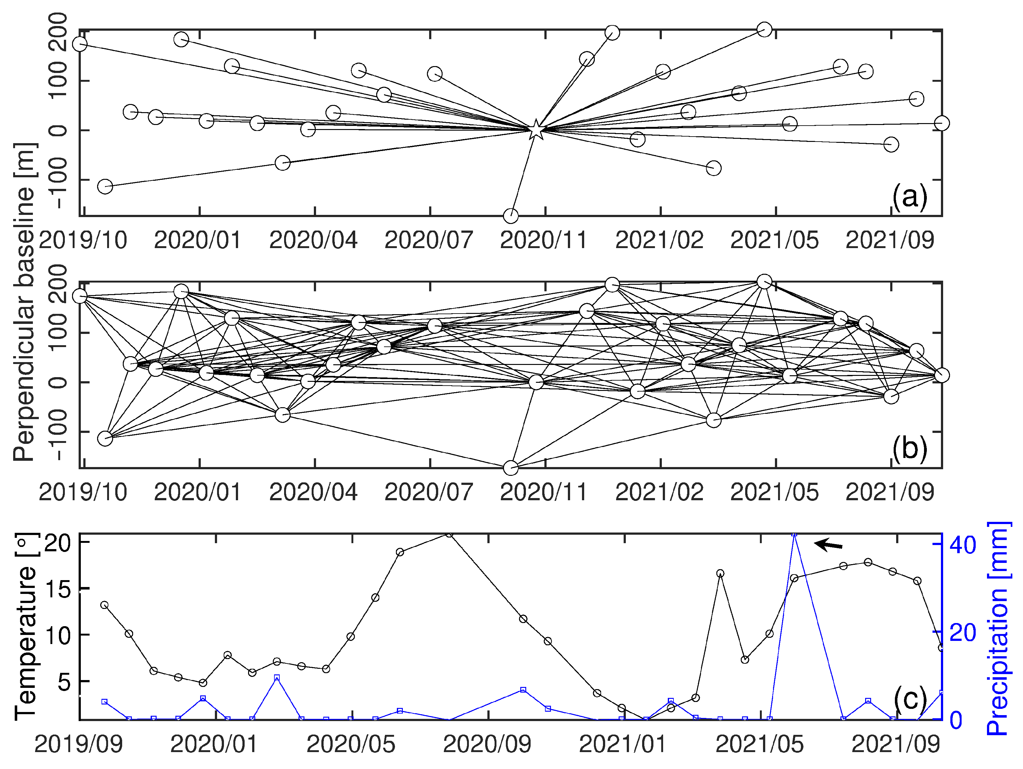
Figure 10d,e as well. For these instances, we also found that as the precipitation dramatically increased to
mm on 5 June 2021 from 0 mm on 14 May 2021, pointed out by the black arrow in
Figure 2c, the values of these two features for IMPs with surface scattering character indicated by the blue square-line rose accordingly, by
dB for
and
dB for
indicated by the black arrow in
Figure 10d,e. We suspect that surface soil reflection of such surface IMPs is enhanced, possibly related to the increase in soil moisture, and temporal evolution of (some) surface IMPs resonates with the changes in precipitation cf. [
66].


