Abstract
This study aims to explore the joint usage of multisource scatterometer measurements in polar sea water and ice discrimination. All radar backscatter measurements from current operating satellite scatterometers are considered, including the C-band ASCAT scatterometer on board the MetOp series satellites, the Ku-band scatterometer on board the HY-2B satellite (HSCAT), and the Ku-band scatterometer on board the CFOSAT satellite (CSCAT). By performing seven experiments that use the same support vector machine (SVM) classifier method but with different input data, we find that the SVM model with all available HSCAT, CSCAT, and ASCAT scatterometer data as inputs gives the best performance. In addition to the SVM outputs, we employ the image erosion/dilation techniques and area growth method to reduce misclassifications of sea water and ice. The sea ice extent obtained in this study shows a good agreement with the National Snow and Ice Data Center (NSIDC) sea ice concentration data from the years 2019 to 2021. More specifically, the sea ice areas are closer to the sea ice areas calculated using 15% as the threshold for NSIDC sea ice concentration data in both Arctic and Antarctic. The sea ice edges acquired by the multisource scatterometer show a close correlation with sea ice edges from the Sentinel-1 Synthetic Aperture Radar (SAR) images. In addition, we found that the coverage of multisource scatterometer data in a half-day is usually above 97%, and more importantly, the sea ice areas obtained on the basis of half-day and daily multisource scatterometer data are very close to each other. The presented work can serve as guidance on the usage of all available scatterometer measurements in sea ice monitoring.
1. Introduction
Polar sea ice is a sensitive indicator and an important driver of global climate change [1]. For instance, the presence of sea ice affects sea surface albedo and reduces the amount of solar radiation absorbed by the Earth’s surface [2]. The spatial and temporal distributions of polar sea ice derived from remote sensing data are important for monitoring global climate change, weather forecasting, and marine transportation [3]. Studies have shown that the sea ice extent is declining in the Arctic, while the trend in the Antarctic is not so clear [4]. In recent years, the study of polar sea ice based on spaceborne active/passive microwave measurements has been receiving increasing attention.
Sea ice extent is a parameter used to describe sea ice conditions and is usually determined on the basis of data from two types of sensors, namely passive microwave radiometers [5] and active microwave scatterometers [6]. Compared to optical remote sensing, microwave sensors are an important means, because they are not seriously affected by sunlight and the atmosphere. The radiometers observe the natural emission from the surface in the range of microwave frequencies, while the scatterometers observe the energy reflected from a transmitted pulse. Microwave scatterometer backscattering characteristics are closely related to the structural properties and composition of sea ice, including dielectric constant, sea ice thickness, temperature, snow thickness, humidity, and salinity, etc. These parameters are related to the type and age of sea ice and external climate change, and also to the type of incident electromagnetic waves (polarization, wavelength, angle of incidence, and azimuth), and these differences are used to distinguish sea ice from open seawater to obtain sea ice coverage and sea ice boundaries. To date, several sources of sea ice product (e.g., sea ice extent, sea ice type) have been developed that are based on space-borne microwave scatterometer data [7,8,9,10].
In 1997, Yueh et al. found that the scattering characteristics at the Ku-band could be used to distinguish sea ice from open seawater [11]. Shortly afterward, Remund and Long developed an algorithm for the automatic identification of sea ice and open water using Ku-band NSCAT (NASA Scatterometer) backscatter measurements [12,13]. This technique is widely known as the Remund/Long-NSCAT (RL-N) algorithm, and it utilizes the backscatter differences in polarization, azimuth, and temporal variation to detect and classify sea ice [14]. However, the accuracy of the RL-N algorithm may be affected by strong winds and summer sea ice melt [15]. In 2014, Remund and Long imporved the RL-N algorithm for Ku-band QuikSCAT/SeaWinds scatterometer data for the classification of sea ice and water. The adapted RL-N algorithm uses an iterative maximum-likelihood classifier with fixed thresholds, and the residual misclassifications are corrected using an image processing technique with the consideration of the patterns of sea ice growth and melting [7].
The radar backscatter data from C-band scatterometers (e.g., scatterometer on board the European Remote Sensing (ERS) satellites or MetOp series satellites) are also widely used in the detection of sea ice extent. For instance, researchers from the French Research Institute for Exploitation of the Sea (IFREMER) used the ERS scatterometer measurements for sea ice detection [16,17]; they proposed two characteristic parameters, which are based on the fact that the scattering anisotropy of sea ice is stronger than that of open seawater, and sea ice backscattering varies less with the incidence angle than does open seawater backscattering. For ice/water discrimination, Breivik et al. proposed a new characteristic parameter utilizing the MetOp-A/ASCAT antenna configuration, which provides three different look angles for the same surface spot [18]. Combing this ASCAT parameter and passive microwave (SSM/I) data, a Bayesian multi-sensor approach was proposed by the Exploitation of Meteorological Satellites (EUMETSAT) Ocean and Sea Ice Satellite Application Facility (OSI SAF) to operationally produce global sea ice edge products [19]. The Royal Netherlands Meteorological Institute (KNMI) developed a Bayesian approach for sea ice detection using radar backscatter measurements from the C-band scatterometers on board the ERS or MetOp satellites [20]; this approach employs geophysical model functions (GMFs) of sea surface wind and sea ice [21,22]. Belmonte Rivas et al. extended the Bayesian sea ice detection algorithm to QuikSCAT data [23], and the new results provided valuable information for the characterization of sea ice during the melting season. By comparison, the RL-N algorithm uses a 4-D hyperspace of measurement vectors, while the KNMI algorithm uses geophysical model functions of the sea ice and open seawater in the original space (i.e., the radar backscatter measurements at different polarization and azimuths).
In addition, there have been increasing studies applying various machine learning algorithms to polar sea ice monitoring in recent years [24,25,26]. Corresponding algorithms are trained based on multi-parameter vectors and models are built for distinguishing sea ice from open seawater. The results all validate that machine learning has a promising ability to detect sea ice.
To date, the space-borne scatterometers operate at either the C-band or the Ku-band. The viewing geometry (e.g., incidence angle, looking azimuth) of the scatterometer is also a major consideration in the application of sea ice monitoring. The C- and Ku-band scatterometers have their own advantages and shortcomings in monitoring polar sea ice. However, previous studies have used either C-band or Ku-band space-borne scatterometer measurements. The performance of sea ice and water discrimination carried out using multiple sources of active microwave measurements remains unexplored. Our study combines a diversity of active microwave measurements in terms of radar frequency (both C and Ku), polarization, azimuth, and incidence angle. It is worth mentioning that the Multidisciplinary drifting Observatory for the Study of Arctic Climate (MOSAiC) expedition provided the unique opportunity to acquire a benchmark data set of multifrequency Ka-, Ku-, X-, C- and L-band in situ microwave scatterometer data (https://www.eumetsat.int/MOSAiC, accessed on 10 March 2023). The MOSAiC expedition aims to characterize the physical properties of the snow and ice cover comprehensively in the central Arctic over an entire annual cycle. In this study, the radar backscatter measurements from multisource satellite scatterometers, including the C-band ASCAT scatterometer on board the MetOp-A, MetOp-B, and MetOp-C satellites, the Ku-band scatterometer on board the HY-2B satellite (HSCAT), and the Ku-band scatterometer on board the CFOSAT satellite (CSCAT) will be jointly used in the detection of polar sea ice extent. This manuscript is structured as follows: In Section 2, the multisource scatterometer data and preprocessing are introduced. In Section 3, the selection and calculation of the characteristic parameters based on the multisource scatterometer data are presented. Then, the sea ice extent mapping and validation are presented in Section 4. Lastly, conclusions are drawn in Section 5.
2. Data Sources and Preprocessing
In this study, radar backscatter measurements from the current operating Ku-band HY-2B/HSCAT and CFOSAT/CSCAT, and C-band ASCAT on board the MetOp-A, MetOp-B, and C satellites are used. More relevant information about the scatterometer data is presented in Table 1.

Table 1.
Information regarding the three scatterometers used in this study.
2.1. Data Sources
2.1.1. Scatterometer data
The HSCAT scatterometer uses two rotating pencil beams, and the normalized radar cross-section () is alternately measured using the horizontally polarized (HH) inner beam and the vertically polarized (VV) outer beam at incidence angles of 41.5° and 48.5°, respectively. Notably, the swath width on the ground of the VV-beam (1800 km) is larger than that of the HH-beam (1400 km). The HSCAT radar backscatter data contained in the level 1B (L1B) data products are used for the period of 1 January 2019–31 December 2021. The resolution of the σ0 data is equal to the size of the “footprint” on the ground, i.e., approximately 25 km × 32 km.
The China–France Oceanography Satellite (CFOSAT), carrying the Ku-band scatterometer (CSCAT), was launched in October 2018. The CSCAT scatterometer uses rotating fan-beams. The data are alternately measured by the HH inner beam and the VV outer beam at incidence angles ranging from 28° to 51° [27]. In this study, the Level 2A (L2A) data products, containing the data corresponding to each wind vector cell, with a grid size of 25 km × 25 km, were used in the period of 1 January 2019–31 December 2021.
The MetOp-A, MetOp-B, and MetOp-C satellites, carrying the C-band ASCAT scatterometer, were successfully launched in 2006, 2012, and 2018, respectively. The ASCAT scatterometer is equipped with three antennas on each side (corresponding to a 500 km swath width on the ground), all of which use VV polarization at incidence angles ranging from 25° to 65°. In addition, the measurements are performed by antennas pointing towards azimuth angles of 45°, 90°, and 135° with respect to the satellite track. The ASCAT data are taken from the L2B products in BUFR (Binary Universal Form for the Representation) format, with resolutions of 12.5 km. In addition, since the differences in among ASCAT-A, ASCAT-B, and ASCAT-C are negligible (i.e., within 0.2 dB), all ASCAT data will be treated as a single data source hereafter.
2.1.2. Sea Ice Concentration Data from NSIDC
The National Oceanic and Atmospheric Administration/National Snow and Ice Data Center (NOAA/NSIDC) climate data record (CDR) of passive microwave sea ice concentration (SIC) dataset from the NSIDC will be used to train our algorithm and validate the results [28]. The CDR SIC is based on two well-established algorithms for sea ice concentration estimation: the NASA Team (NT) algorithm and the NASA Bootstrap (BT) algorithm. The CDR algorithm mixes the NT and BT outputs by selecting higher SIC values for each grid cell. The NSIDC SIC data are provided in a polar stereographic projection at a grid cell size of 25 km × 25 km for the northern and southern hemispheres separately.
2.1.3. SAR Imagery
SAR images provide geographic information on sea ice with high spatial resolution and will be used to verify the results of the sea ice edges in localized areas [29,30]. The polar view website (www.polarview.aq, accessed on 10 March 2023) provides full-resolution SAR image data observed by Sentinel-1 and RADARSAT-2 over the previous 30 days. In addition, the SAR images are used as a polar stereographic projection, which is consistent with the projection of sea ice maps. The Sentinel-1 SAR images with 5 m resolution will be used to verify the boundary of open seawater and ice.
2.2. Data Preprocessing
In this study, the radar backscatter () measurements from the HSCAT, ASCAT, and CSCAT scatterometers are first projected onto polar ice maps with a resolution of 25 km. The sizes of the Arctic and Antarctic ice maps are 448 × 304 and 332 × 316, respectively. Figure 1 shows the number of ASCAT data in each pixel of the (a) Antarctic and (b) Arctic ice maps on 4 January 2020. The overlying black lines are the land boundary. We can clearly see that the number of observations is relatively lower at lower latitudes.
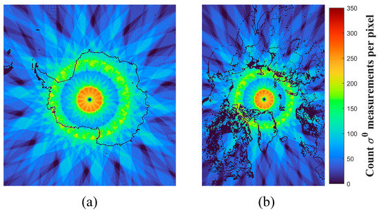
Figure 1.
A number of ASCAT measurements in (a) Antarctic and (b) Arctic areas on 4 January 2020. The coastlines are overlaid in black, while the color bar represents the count of measurements in each pixel. The image sizes of the Arctic and Antarctic ice maps are 448 × 304 and 332 × 316, respectively.
In addition, radar backscatters from ASCAT and CSCAT scatterometers are measured at various incidence angles (as shown in Table 1). The backscattering characteristics of sea water and ice have different responses to incidence angle. Thus, the dependence of data on incidence angle can also be used as a characteristic parameter in the classification of sea water and ice. In practice, a linear function of incidence angle (θ) is usually used to express the incidence angle dependence [12]:
where is in decibels; denotes the backscatter coefficients at an incidence angle of 40; and is the slope of the linear function and gives the dependence of the backscattering coefficients on the incidence angle.
3. Characteristic Parameters for Sea Ice Monitoring
In this study, we aim to explore the merits of combing C-band and Ku-band scatterometer measurements in the application of sea water and ice classification. However, the HSCAT, CSCAT, and ASCAT scatterometers operate at different viewing geometries, in terms of incidence angle and antenna looking direction. Thus, we could not extract the same characteristic parameters from every scatterometer. Nevertheless, we propose using seven characteristic parameters, including horizontal and vertical polarization backscatter measurements ( and ), standard deviations of horizontal and vertical polarization measurements ( and ), polarization ratio (), the dependence of on incidence angle (, as defined in Equation (1)), and the ratio of backscatter measurements between C-band and Ku-band (named band ratio ()). The availability of these parameters from the scatterometers is listed in Table 2. Figure 2 shows the normalized distribution of sea ice and open seawater in the Antarctic region for each parameter. These distributions are counted from December 2019 to February 2020 based on multisource scatterometer measurements.
Table 2.
Information on the characteristic parameters of multisource scatterometer.
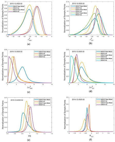
Figure 2.
Normalized distribution of the characteristic parameters over open seawater and ice in the Antarctic; the period over which statistics were obtained was from December 2019 to February 2020. (a) (dB), (b) (dB), (c) standard deviations of HH measurements, (dB), (d) standard deviations of VV measurements, (dB), (e) polarization ratio of backscatter measurements , (f) backscatter dependence on incidence angle and (g) band ratio of VV backscatter measurements, .
Comparing the horizontal and vertical polarized backscatter measurements of sea ice and sea water, different scattering mechanisms play a role [3,7]. Over sea water, backscatter coefficients are primarily dependent on wind speed. The backscatter coefficients are usually quite different between sea water under low wind speed (<5 m/s) conditions and sea ice. For a given measuring geometry (e.g., HSCAT), the backscatter coefficients of sea ice are usually stronger than those of water; see the yellow and purple curves shown in Figure 2a.
In contrast to other active radar systems (e.g., SAR), scatterometers can measure the same ground area at multiple azimuth angles; this was originally required by the sea surface wind retrieval mission. It has been demonstrated that the azimuthal modulation is much smaller over polar sea ice than over open seawater [31,32]. The daily standard deviations of horizontal and vertical polarization backscatter ( and ) can represent the azimuthal and temporal dependences of surface backscatter, as shown in Figure 2c,d.
In previous studies, polarization ratios obtained on the basis of dual-polarization radar measurements from the SEASAT scatterometer, the QuikSCAT/SeaWinds scatterometer, and the HY-2A scatterometer have been used for the identification of sea ice and open seawater [3,11,12,13,14]. In this study, the is defined as the ratio of and , i.e.,. is sensitive to surface-scattering mechanisms. For example, on a calm seawater surface, is larger than . For rough surface dielectric layers with randomly oriented scatterers such as ice or snow, multiple reflections of the incident radiation tend to depolarize it. Therefore, and are closer. As shown in Figure 2e, is usually higher over sea ice than that over sea water. However, the increased surface roughness of sea water caused by high sea surface winds may lead to a higher .
Since the ASCAT and CSCAT scatterometers are able to measure the same pixel of the sea ice map at various incidence angles, the dependence of measurements on incidence angle can be represented by the slope (denoted as ) of a linear fitting function. In general, the backscattering amplitude of sea water decreases more rapidly with increasing incidence angle than that of sea ice [13]. This is in line with the plots shown in Figure 2f, i.e., most slope values are negative, and the slopes of sea water are relatively steeper than those of sea ice.
In this study, we propose a new parameter named band ratio (). is defined as the ratio of vertically polarized backscatter measurements from the Ku-band to that from C-band. More specifically, is the ratio of the CSCAT measurement to the ASCAT measurement. As shown in Figure 2g, the of open water is mostly larger than that of sea ice.
4. Sea Ice Extent Mapping and Validation
4.1. SVM Sea Ice and Water Discrimination Algorithm
In this study, the support vector machine (SVM) classifier will be used to discriminate between sea ice and water. The SVM classifier is a supervised learning algorithm that converts the input parameter vector into a high-dimensional space and finds the optimal linear classification surface in this new high-dimensional space to solve nonlinear problems. An increasing number of studies are being published using the SVM method to solve problems relating to remote sensing image classification [30,33,34].
In order to train the SVM classifier, the NSIDC SIC data from NSIDC are used as a priori knowledge of sea water and ice. If the SIC is greater than or equal to 15%, the corresponding pixels of ice maps are identified as sea ice, while if the SIC is less than 15%, the corresponding pixels of ice maps are identified as sea water. The training dataset was collected during the year 2020, and we randomly picked 20,000 samples for both water and ice per month. A set of characteristic parameters were derived from multiple scatterometer data containing a priori information on sea ice and open water (as shown in Table 2), where the sample dataset D can be expressed as follows:
where represents the input samples, which consist of features for classification, and is the class label of . In this study, there are only two categories of sea ice and seawater, i.e., is set to +1 and −1. SVM is used to find an optimal classification hyperplane in high-dimensional space, denoted by Equation (3):
At this point, the maximum classification interval algorithm can be formulated as Equation (4):
Equation (4) can be solved using the Lagrange multiplier method. That is, by first adding Lagrange multipliers to each constraint, the Lagrange function for this problem can be rewritten as Equation (5):
The optimal solution for and the optimal solution for are obtained using the sequential minimum optimization algorithm once, for any sample, the output of the classification has been determined by the decision function. The nonlinear change in the transformation from a low-dimensional vector to a high-latitude space is achieved by defining appropriate inner product functions, i.e., kernel functions. In this study, the Gaussian kernel function is chosen. Figure 3 shows the flowchart of sea ice monitoring using the SVM classifier with multisource scatterometer measurements used in this study.
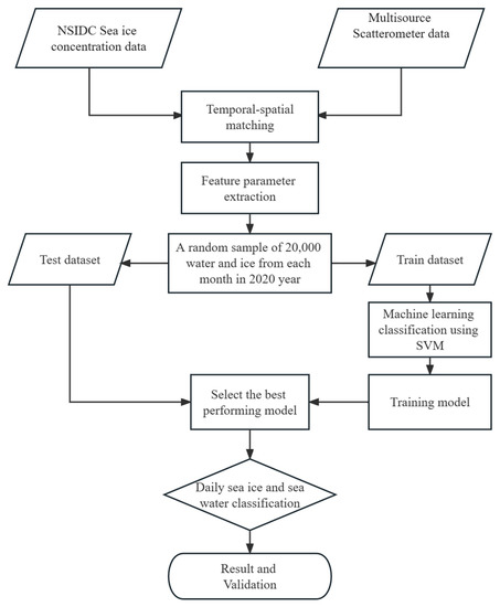
Figure 3.
The flowchart of sea ice monitoring based on SVM classifier with multisource scatterometer measurement.
4.2. SVM Model Experiments
In order to identify the best scheme for combining HSCAT, CSCAT, and ASCAT data, we performed seven SVM model experiments (as shown in Table 3). The experiments used the same SVM classifier method, but with different input data, and the experiments were divided into three categories for the sake of comparison. To evaluate the performance of the experiments, 100,000 samples were randomly picked as the test dataset for each experiment.
Table 3.
Categories of SVM model experiments.
Category 1 compares the results from HSCAT, ASCAT, and joint usage of HSCAT and ASCAT. For HSCAT data, four parameters (the same as the well-known QuikSCAT RL-N algorithm) are used. For ASCAT data, three parameters are used. In addition, to make the results more comparable, we only work on the pixels for which both HSCAT and ASCAT data are available.
In category 2, the results from CSCAT, ASCAT, and joint usage of CSCAT and ASCAT are compared. Both CSCAT and ASCAT are able to provide incidence-angle-dependent backscatter measurements, thus making available the parameters of and .
Category 3 assembles all of the parameters from the HSCAT, CSCAT, and ASCAT measurements. In categories 1 and 2, the same pixels of daily sea ice maps were used for different experiments. Thus, we are solving the same problem (sea water and ice discrimination) using the same SVM method, but with different model inputs.
Figure 4a,b show the overall accuracy (OA) of the SVM model derived from the test set in the Arctic for Antarctic, respectively. It can be observed that the OA of the SVM model with only ASCAT as inputs (i.e., experiments II and V) is clearly lower than that of the other models. The OA of the models with data from a single Ku-band (experiments I and IV) scatterometer as inputs is higher than the models with data from a single C-band scatterometer as inputs. The model with only CSCAT data as inputs (experiment IV) performs slightly better than the model with only HSCAT data as inputs (experiment I). For model experiments with joint usage of scatterometer data (experiments III, VI, and VII), the OAs of models with both Ku-band and C-band scatterometer data are higher than those of models using Ku-band or C-band scatterometer data alone. It is noted that, with sufficient training samples, the SVM model with all available scatterometer data as inputs show the best performance among all seven model experiments.
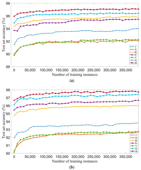
Figure 4.
The overall accuracy of different SVM model experiments in (a) Arctic and (b) Antarctic regions.
In summary, the SVM model (i.e., experiment VII) in which all available characteristic parameters from HSCAT, CSCAT, and ASCAT measurements were used as inputs demonstrated the best performance and will be used hereafter for sea water and ice discrimination.
4.3. Evaluation of Sea Ice Distribution Model Precision
A more detailed evaluation of the selected SVM model (i.e., experiment VII), which inputs all available characteristic parameters from HSCAT, CSCAT, and ASCAT measurements, is performed. Again, we use NSIDC SIC data as reference data. The evaluation indicators include accuracy, precision, recall, and F1 score. The accuracy gives the overall prediction accuracy of the model. The precision is defined as the proportion of correctly predicted samples to total samples. The recall represents the probability of the samples being correctly predicted. The F1 score is an index used to measure the accuracy of a classification model that takes into account both the precision and recall of the classification model.
It should be noted that, in the confusion matrix, the true positive (TP), true negative (TN), false positive (FP) and false negative (FN) is defined differently for each type. Therefore, the values of any precision, recall and F1 scores can be defined as follows:
Figure 5 and Figure 6 show the time series of sea ice monitoring model evaluation indicators for the Arctic and Antarctic for the years 2019 to 2021, respectively. Table 4 presents the average classification accuracy, where an overall accuracy of 98.41% was obtained for the Antarctic and 97.15% for the Arctic; the accuracy of the model in the Antarctic region is higher than in the Arctic. In the Arctic, the precision for sea ice was slightly lower in summer and early autumn than in the other seasons. Similarly, the precision for open water in summer was significantly lower than that in other seasons in the Antarctic. This may be due to the fact that melting sea ice in summer increases the content of seawater in sea ice and increases its dielectric constant [6,13], causing the backscattering coefficient of sea ice to be similar to that of seawater, meaning that the model has a lower sea ice identification rate in summer.
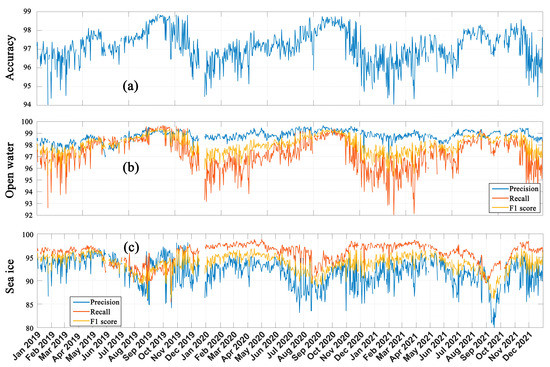
Figure 5.
Time series of model performance in Arctic for the period from 2019 to 2021: (a) overall accuracy; and precision, recall and F1 scores for (b) open water and (c) sea ice.
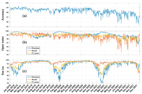
Figure 6.
Time series of model performance in the Antarctic for the period from 2019 to 2021: (a) overall accuracy; and precision, recall and F1 scores for (b) open water and (c) sea ice.
Table 4.
Summary of averaged classification accuracies obtained using an SVM classifier in the Arctic and Antarctic from 2019 to 2021.
Figure 7a shows an example of the sea water and ice discrimination results (26 September 2020) using the trained SVM model with multisource scatterometer data as inputs. The NSIDC SIC data on the same date are shown in Figure 7c. Overall, the sea water and ice are well distinguished. However, some pixels in the open sea, closed ice, or near the ice edge are misclassified. Therefore, a residual classification error correction processing is needed to improve the outputs of the SVM model.
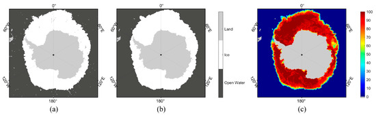
Figure 7.
Antarctic Sea ice maps on 26 September 2020 (gray parts in center represent land): (a) SVM model outputs; (b) after misclassification reduction processing; (c) NSIDC sea ice concentration.
4.4. Reduction of Residual Classification Errors
Because of the presence of strong winds or other physical mechanisms, the SVM model outputs can contain some misclassifications. For instance, some of the open seawater pixels are misclassified as sea ice, and sea ice pixels are misclassified as open seawater, as shown in Figure 7a. In this study, we employ the area growth technique (see [13]) to reduce the number of misclassifications. The area growth technique starts with a small region known to be within the ice area and expands this region until it reaches the outer edge of the ice region and cannot be expanded further. This eliminates pixels in the sea ice region misclassified as open seawater. Conversely, growth can be performed from the outer edge towards the inner region until the sea ice edge is reached. This eliminates pixels within the open seawater region that are misclassified as sea ice. Once area growth is complete, there may be some residual noise at the sea ice edge, which is where the “indentation” or “squeeze” observation error needs to be resolved using image erosion and dilation techniques [35]. In this study, 100 km per day was used as the maximum sea ice growth or ablation rate threshold between two consecutive days and produced good results in terms of eliminating misclassification for sea ice growth and ablation. The SVM model outputs following misclassification correction are shown in Figure 7b. It is clear that most of the misclassified pixels in the closed sea ice and the open sea have been corrected.
4.5. Sea Ice Mapping and Validation
Using the sea water and ice discrimination method presented above, we processed the daily Arctic and Antarctic daily ice maps from 1 January 2019 to 31 December 2021. Figure 8 shows the geographical distribution of sea ice results derived from a multisource scatterometer for some days in the year 2020. In Figure 8a–d, the Antarctic Sea ice images for minimum sea ice extent (20 Feb), expansion (10 Jun), maximum sea ice extent (26 Sep), and melt phase (09 Dec) demonstrate the seasonal variation in the ice pack. In Figure 8e–h, the Arctic Sea ice images for the maximum sea ice extent (01 Mar), retreat (13 May), minimum sea ice extent (13 Sep), and growth (10 Nov) are presented. In addition, the polynyas off the Antarctic coast can also be clearly detected, as shown in Figure 8d for the date of 9 Dec 2020.
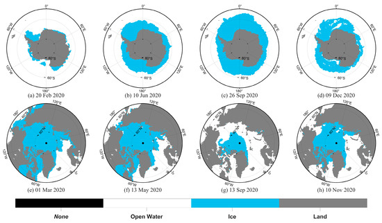
Figure 8.
Example daily polar sea ice extent obtained on the basis of multisource scatterometer data. Gray pixels represent land; white pixels represent water; blue pixels represent sea ice; and the black hole in the Arctic is due to there being no coverage by scatterometers.
4.5.1. Comparison with NSIDC SIC
In this study, sea ice extent data retrieved using our SVM-based algorithm are compared with the NSIDC SIC operational products. As described in Section 2, we are working on the same polar projection and spatial resolution as the NSIDC SIC products. The daily polar sea ice extents from the SVM model and the NSIDC CDR ice extents (with SIC thresholds of 15% and 30%) from January 2019 to December 2022 are shown in Figure 9 and Figure 10, respectively. The seasonal variations in ice extent can be clearly observed in the multisource scatterometer data, which show synchronous changes with NSIDC CDR ice extent. Furthermore, we calculated the mean absolute differences (MAD) and standard deviation (SD) of the sea ice extent for this comparison, and some quantitative details are given in Table 5. In Table 5, JFM represents January, February, and March; AMJ represents April, May, and June; JAS represents July, August, and September; OND represents October, November, and December. Sea ice extents from the multisource scatterometer data are closer to the NSIDC SIC 30% sea ice extent during OND in the Arctic, and closer to the NSIDC SIC 15% ice extent during the other phases. In the Antarctic, the sea ice extents determined on the basis of the multisource scatterometer data are closer to the NSIDC SIC 30% sea ice extent during the AMJ and JAS periods, while the MAD and SD results during the JFM and OND periods show good agreement with the NSIDC SIC 15% sea ice extent. We find that in the Antarctic or Arctic, the sea ice extent obtained by the multisource scatterometer is overestimate the NSIDC SIC 15% and 30% sea ice extent from the late stages of sea-ice ablation to the beginning of the sea-ice growth phase. Our results may detect more low-concentration sea ice.
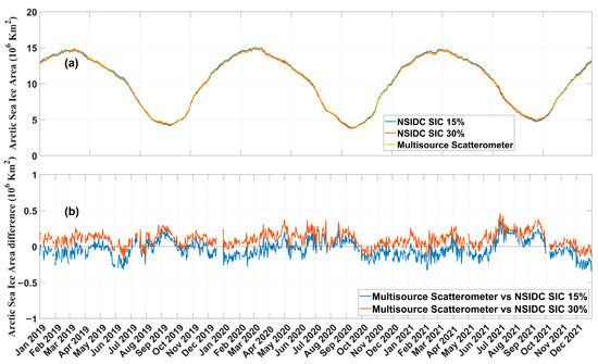
Figure 9.
The validation results of the Arctic from 2019 to 2021; (a) daily sea ice area for NSIDC SIC 15% ice extent (blue line), NSIDC SIC 30% ice extent (red line), and multisource scatterometer (yellow line), respectively, and (b) sea ice area difference between multisource scatterometer and NSIDC SIC 15% (blue line), and between multisource scatterometer and NSIDC SIC 30% (red line).
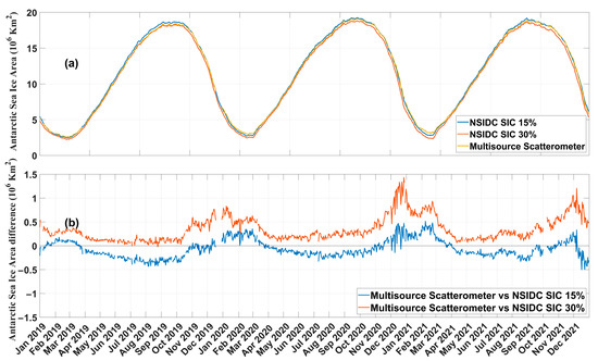
Figure 10.
The validation results for the Antarctic from 2019 to 2021: (a) daily sea ice area for NSIDC SIC 15% ice extent (blue line), NSIDC SIC 30% ice extent (red line), and multisource scatterometer (yellow line), respectively, and (b) sea ice area difference between multisource scatterometer and NSIDC SIC 15% (blue line), and between multisource scatterometer and NSIDC SIC 30% (red line).
Table 5.
Statistics of the comparisons between multisource scatterometer and NSIDC SIC 15% and 30% sea ice extents for different periods: All refers to all data; JFM is for the months January, February, and March; AMJ is for months April, May, and June; JAS is for months July, August, and September; and OND is for months October, November, and December.
As listed in Table 5, our results are closer to the NSIDC SIC data with a threshold of 15% in most seasons. Overall, the differences in sea ice extent between our results and the NSIDC SIC 15% are smaller in both the Arctic and Antarctic. The MAD and SD are 0.121 and 0.119 million km2, respectively, in the Arctic, while these are 0.166 and 0.146 million km2, respectively, in the Antarctic.
4.5.2. Comparison with SAR
Sentinel-1 SAR images have a high spatial resolution (5 m), and open seawater and ice can be easily distinguished visually. SAR images are usually used for evaluating the edge of open water and closed ice. In this study, four Sentinel-1 SAR images (horizontally polarized at C-band) were used, and the results are shown in Figure 11. To facilitate comparison, the sea ice edge lines from the multisource scatterometer data and the NSIDC SIC 15% sea ice overlapped. In the SAR images, the backscattering amplitude of the sea ice is generally stronger than that of the sea water, and, as a result, the pixels of sea ice are brighter than those of water.
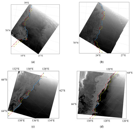
Figure 11.
Sentinel-1 SAR images showing sea water and ice distributions. Sea ice edge lines from the multisource scatterometer data (red lines) and NSIDC SIC 15% sea ice (yellow lines) are overlapped, with the blue line being the common overlay sea ice edge line. The image acquisition dates were: (a) 4 December 2021, (b) 24 December 2021, (c) 29 November 2021, and (d) 18 December 2021.
Figure 11a,b show the distribution of sea ice in the local region in the Arctic on 4 December and 24 December 2021. Figure 11c,d show the local surface types in the Antarctic region on 29 November and 18 December 2021. It should be noted that SAR images give a view of sea water and ice at a single point in time, while our results and NSIDC SIC products are determined on the basis of satellite passes over the course of a single day. From Figure 11a,b, it can be seen that the multisource scatterometer sea ice boundary fits more closely to the SAR image sea ice boundary than the NSIDC SIC 15% sea ice boundary, while Figure 11c,d show that the SAR image sea ice boundary lies between the multisource scatterometer sea ice boundary and the NSIDC SIC 15% sea ice boundary, and the vast majority of the sea ice boundaries in Figure 11 are overlapping. Despite the lower-resolution conditions, it can be seen that the sea ice edges from the multisource scatterometer data are in good agreement with the SAR images.
4.5.3. Test for Half-Day Retrievals
Since the multi-source scatterometer offers more complete coverage of observations compared to the single-source scatterometer, thus resulting in a larger number of observations being acquired in the projected grid of the Arctic and Antarctic, it would therefore be possible to shorten the time interval to 12 h (separation at noon) in an attempt to retrieve half-day sea ice extents on the basis of multisource scatterometer data.
We selected the multisource scatterometer data for October 2020 to try this out. In this section, we exclude polar regions over land and the polar hole (no scatterometer data coverage). In Figure 12a and Figure 13a, it can be seen that the data coverages of multisource scatterometer data (i.e., containing at least one scatterometer measurement within the grid cell) as a percentage are above 97% at both half-day and one-day time intervals in both the Antarctic and the Arctic. In Figure 12b and Figure 13b, it can be observed that the half-day sea ice area is in good agreement with the daily sea ice area. The MAD of differences between daily and half-day sea ice areas are 0.088 and 0.131 million km2 for the Arctic and Antarctic, respectively.
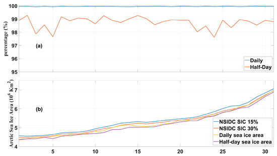
Figure 12.
Comparison of acquisition of data at daily and half-day time intervals in the Artic for October 2020: (a) data coverage; (b) sea ice area.
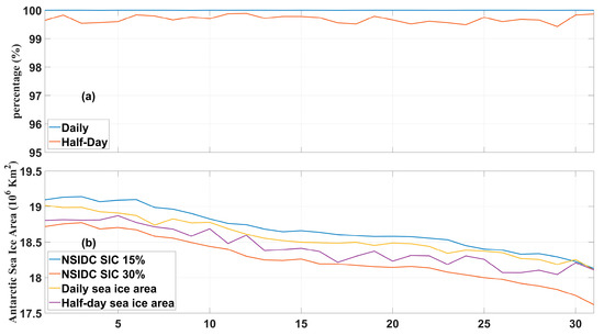
Figure 13.
Comparison of acquisition of data at daily and half-day time intervals in the Antarctic for October 2020: (a) data coverage; (b) sea ice area.
5. Conclusions
In this study, we performed sea ice and water discrimination based on multisource scatterometer measurements using an SVM model. In contrast to previous studies, multisource scatterometer measurements from the C-band MetOp/ASCAT, Ku-band HY-2B/SCAT, and CFOSAT/CSCAT were used in combination. The scatterometer measurements were used to determine characteristic parameters, including polarization ratio (/), horizontal and vertical polarization backscatter measurements ( and ), the standard deviations of horizontal and vertical polarization measurements ( and ), the dependence of on incidence angle (), and the newly proposed band ratio (/).
SVM is a supervised classification method that can handle linear, nonlinear, and high-dimensional samples and produce good generalizability. Therefore, the SVM classifier was selected for sea ice monitoring in this study. In order to determine the best scheme for the use of these multisource scatterometer data, seven SVM model experiments (see Table 3) were performed. We found that the SVM model using all available scatterometer data as inputs performed best among the seven model experiments. In addition to the SVM outputs, we employed image erosion/dilation techniques and the area growth method to reduce the number of misclassifications of sea water and ice. Using our sea water and ice discrimination algorithm, we produced sea ice products for the years from 2019 to 2021; and the results obtained for sea ice extent and edges were verified against NSIDC SIC and Sentinel-1 SAR images. The verification results show that the multisource scatterometer sea ice extent lay between the NSIDC SIC 15% and 30% sea ice extent, and there was good agreement with the NSIDC SIC 15% sea ice extent while showing similar seasonal trends to the sea ice area of the NSIDC SIC data. The multisource scatterometer sea ice edge showed a good correlation with the sea ice edge determined on the basis of the SAR images. We also tested the possibility of providing shorter-time-interval (i.e., half-day) sea ice products on the basis of multi-source scatterometer data, and we found that the half-day coverage was above 97%, while half-day sea ice area was in good agreement with the daily sea ice area.
In conclusion, this study verified the capability of multisource scatterometer measurements for the monitoring of polar sea ice. In the near future, the ability of scatterometer measurements for the monitoring of polar sea ice will be enhanced, as a result of the enhanced configurations of recently launched (FY-3E/WindRAD) and planned scatterometers in terms of radar frequency, polarization, incidence angle, and spatial resolution. Studies on sea ice type classification in polar areas using multisource scatterometers will be introduced in our future work.
Author Contributions
Conceptualization, C.X. and Z.W.; methodology, C.X. and Z.W.; software, C.X.; validation, Z.W. and C.X.; formal analysis, C.X.; investigation, C.X. and Z.W.; resources, Z.W.; data curation, C.X. and Z.W.; writing—original draft preparation, C.X. and Z.W.; writing—review and editing, Z.W., X.Z., W.L., Y.H. and C.X.; visualization, C.X.; supervision, Z.W., W.L., X.Z. and Y.H.; project administration, Z.W. and Y.H.; funding acquisition, Z.W. All authors have read and agreed to the published version of the manuscript.
Funding
This research was supported by the National Key Research and Development Program of China (2021YFC2803301).
Data Availability Statement
Not applicable.
Acknowledgments
The authors would like to thank the Chinese National Satellite Ocean Application Services (NSOAS) for providing the CSCAT and HSCAT data, the Royal Netherlands Meteorological Institute (KNMI) for providing the ASCAT data, the National Snow and Ice Data Center (NSIDC) for providing sea ice concentration products, and the Polar View Website for providing SAR image data used in comparison. The authors would also like to thank the editor and reviewers whose insightful comments offered significant improvements to this paper.
Conflicts of Interest
The authors declare no conflict of interest.
References
- Cavalieri, D.J.; Parkinson, C.L. Antarctic sea ice variability and trends, 1979–2006. J. Geophys. Res. 2008, 113, C07004. [Google Scholar] [CrossRef]
- Curry, J.A.; Schramm, J.L.; Ebert, E.E. Sea ice-albedo climate feedback mechanism. J. Clim. 1995, 8, 240–247. [Google Scholar] [CrossRef]
- Li, M.; Zhao, C.; Zhao, Y.; Wang, Z.; Shi, L. Polar sea ice monitoring using HY-2A scatterometer measurements. Remote Sens. 2016, 8, 688. [Google Scholar] [CrossRef]
- IPCC (Intergovernmental Panel on Climate Change). Climate Change 2021: The Physical Science Basis. The Working Group I Contribution to the Sixth Assessment Report. 2021. Available online: https://www.ipcc.ch/report/sixth-assessment-report-working-group-i/ (accessed on 10 March 2023).
- Tikhonov, V.V.; Raev, M.D.; Sharkov, E.A.; Boyarskii, D.A.; Repina, I.A.; Komarova, N.Y. Satellite microwave radiometry of sea ice of polar regions: A review. Atmos. Ocean. Phys. 2016, 52, 1012–1030. [Google Scholar] [CrossRef]
- Long, D.G. Polar applications of spaceborne scatterometers. IEEE J. Sel. Top. Appl. Earth. Obs. Remote Sens. 2016, 10, 2307–2320. [Google Scholar] [CrossRef]
- Remund, Q.P.; Long, D.G. A decade of QuikSCAT scatterometer sea ice extent data. IEEE Trans. Geosci. Remote Sens. 2014, 52, 4281–4290. [Google Scholar] [CrossRef]
- Rivas, M.B.; Verspeek, J.; Verhoef, A.; Stoffelen, A. Bayesian sea ice detection with the advanced scatterometer ASCAT. IEEE Trans. Geosci. Remote Sens. 2012, 50, 2649–2657. [Google Scholar] [CrossRef]
- Lindell, D.B.; Long, D.G. Multiyear Arctic sea ice classifification using OSCAT and QuikSCAT. IEEE Trans. Geosci. Remote Sens. 2016, 54, 167–175. [Google Scholar] [CrossRef]
- Zhang, Z.; Yu, Y.; Li, X.; Hui, F.; Cheng, X.; Chen, Z. Arctic sea ice classification using microwave scatterometer and radiometer data during 2002-2017. IEEE Trans. Geosci. Remote Sens. 2019, 57, 5319–5328. [Google Scholar] [CrossRef]
- Yueh, S.H.; Kwok, R.; Lou, S.-H.; Tsai, W.-Y. Sea ice identifification using dual-polarized Ku-band scatterometer data. IEEE Trans. Geosci. Remote Sens. 1997, 35, 560–569. [Google Scholar] [CrossRef]
- Remund, Q.P.; Long, D.G. Automated Antarctic ice edge detection using NSCAT data. In Proceedings of the 1997 IEEE International, Geoscience and Remote Sensing (IGARSS’97), Remote Sensing—A Scientific Vision for Sustainable Development, Singapore, 3–8 August 1997; pp. 1841–1843. [Google Scholar]
- Remund, Q.P.; Long, D.G. Sea ice extent mapping using Ku band scatterometer data. J. Geophys. Res. Oceans 1999, 104, 11515–11527. [Google Scholar] [CrossRef]
- Remund, Q.P.; Long, D.G. Sea ice mapping algorithm for QuikSCAT and SeaWinds. In Proceedings of the 1998 IEEE International, Geoscience and Remote Sensing Symposium Proceedings, 1998. (IGARSS’98), Seattle, WA, USA, 6–10 July 1998; pp. 1686–1688. [Google Scholar]
- De Abreu, R.; Wilson, K.; Arkett, M.; Langlois, D. Evaluating the use of QuikSCAT data for operational sea ice monitoring. In Proceedings of the 2002 IEEE International Geoscience and Remote Sensing Symposium (IGARSS’02), Toronto, ON, Canada, 24–28 June 2002; pp. 3032–3033. [Google Scholar]
- Gohin, F.; Cavanie, A. A first try at identifification of sea ice using the three beam scatterometer of ERS-1. Int. J. Remote Sens. 1994, 15, 1221–1228. [Google Scholar] [CrossRef]
- Cavanie, A.; Gohin, F.; Quilfen, Y.; Lecomte, P. Identifification of sea ice zones using the AMI wind: Physical bases and applications to the FDP and CERSAT processing chains. In Proceedings of the 2nd ERS-1 Symposium, Hamburg, Germany, 11–14 October 1993; pp. 1009–1012. [Google Scholar]
- Breivik, L.A.; Eastwood, S.; Lavergne, T. Use of C-band scatterometer for sea ice edge identifification. IEEE Trans. Geosci. Remote Sens. 2012, 50, 2669–2677. [Google Scholar] [CrossRef]
- Aaboe, S.; Down, E.J.; Eastwood, S. Algorithm Theoretical Basis Document for the Global Sea-Ice Edge and Type Product; Norwegian Meteorological Institute: Blindern, Norway, 2021; Available online: https://osisaf-hl.met.no/sites/osisaf-hl/files/baseline_document/osisaf_cdop3_ss2_atbd_sea-ice-edge-type_v3p4.pdf (accessed on 10 March 2023).
- Haan, S.D.; Stoffelen, A. Ice Discrimination Using ERS Scatterometer, EUMETSAT, Darmstadt, Germany, Tech. Rep. SAF/OSI/KNMI/TEC/TN/120. Available online: http://www.knmi.nl/publications/ (accessed on 10 March 2023).
- Otosaka, I.; Rivas, M.B.; Stoffelen, A. Bayesian Sea Ice Detection with the ERS Scatterometer and Sea Ice Backscatter Model at C-Band. IEEE Trans. Geosci. Remote Sens. 2018, 56, 2248–2254. [Google Scholar] [CrossRef]
- Rivas, M.B.; Otosaka, I.; Stoffelen, A.; Verhoef, A. A scatterometer record of sea ice extents and backscatter: 1992–2016. Cryosphere 2018, 12, 2941–2953. [Google Scholar] [CrossRef]
- Rivas, M.B.; Stoffelen, A. New Bayesian algorithm for sea ice detection with QuikSCAT. IEEE Trans. Geosci. Remote Sens. 2011, 49, 1894–1901. [Google Scholar] [CrossRef]
- Ren, Y.; Li, X.; Yang, X.; Xu, H. Development of a dual-attention U-Net model for sea ice and open water classification on SAR images. IEEE Trans. Geosci. Remote Sens. Lett. 2021, 19, 1–5. [Google Scholar] [CrossRef]
- Zhang, J.; Zhang, W.; Hu, Y.; Chu, Q.; Liu, L. An Improved Sea Ice Classification Algorithm with Gaofen-3 Dual-Polarization SAR Data Based on Deep Convolutional Neural Networks. Remote Sens. 2022, 14, 906. [Google Scholar] [CrossRef]
- Zhai, X.; Wang, Z.; Zheng, Z.; Xu, R.; Dou, F.; Xu, N.; Zhang, X. Sea Ice Monitoring with CFOSAT Scatterometer Measurements Using Random Forest Classifier. Remote Sens. 2021, 13, 4686. [Google Scholar] [CrossRef]
- Lin, W.; Dong, X.; Portabella, M.; Lang, S.; He, Y.; Yun, R.; Wang, Z.; Xu, X.; Zhu, D.; Liu, J. A perspective on the performance of the cfosat rotating fan-beam scatterometer. IEEE Trans. Geosci. Remote Sens. 2019, 57, 627–639. [Google Scholar] [CrossRef]
- Meier, W.N.; Fetterer, F.; Windnagel, A.K.; Stewart, J.S. NOAA/NSIDC Climate Data Record of Passive Microwave Sea Ice Concentration, Version 4; NOAA/NSIDC: Boulder, CO, USA, 2021. [Google Scholar] [CrossRef]
- Dierking, W. Sea ice monitoring by synthetic aperture radar. Oceanography 2013, 26, 100–111. [Google Scholar] [CrossRef]
- Li, X.; Sun, Y.; Zhang, Q. Extraction of Sea Ice Cover by Sentinel-1 SAR Based on Support Vector Machine with Unsupervised Generation of Training Data. IEEE Trans. Geosci. Remote Sens. 2021, 59, 3040–3053. [Google Scholar] [CrossRef]
- Remund, Q.; Early, D.; Long, D. Azimuthal Modulation of Ku-Band Scatterometer Sigma-0 over the Antarctic; MERS: Provo, UT, USA, 3 July 1997. [Google Scholar]
- Early, D.S.; Long, D.G. Azimuthal modulation of C-band scatterometer σ0 over Southern Ocean sea ice. IEEE Trans. Geosci. Remote Sens. 1997, 35, 1201–1209. [Google Scholar] [CrossRef]
- Chapelle, O.; Haffner, P.; Vapnik, V.N. Support vector machines for histogram-based image classification. IEEE Trans. Neural Netw. 1999, 10, 1055–1064. [Google Scholar] [CrossRef] [PubMed]
- Liu, H.; Guo, H.; Zhang, L. SVM-Based Sea Ice Classification Using Textural Features and Concentration From RADARSAT-2 Dual-Pol ScanSAR Data. IEEE J. Sel. Top. Appl. Earth. Obs. Remote Sens. 2015, 8, 1601–1613. [Google Scholar] [CrossRef]
- Russ, J.C. The Image Processing Handbook; CRC Press: Boca Raton, FL, USA, 2015. [Google Scholar]


Disclaimer/Publisher’s Note: The statements, opinions and data contained in all publications are solely those of the individual author(s) and contributor(s) and not of MDPI and/or the editor(s). MDPI and/or the editor(s) disclaim responsibility for any injury to people or property resulting from any ideas, methods, instructions or products referred to in the content. |
© 2023 by the authors. Licensee MDPI, Basel, Switzerland. This article is an open access article distributed under the terms and conditions of the Creative Commons Attribution (CC BY) license (https://creativecommons.org/licenses/by/4.0/).