Abstract
Since launch, the Ku-band rotating fan-beam scatterometer onboard the China–France Oceanography Satellite (CFOSAT) has provided valuable sea surface wind measurements for more than four years. The performance of CFOSAT scatterometer (CSCAT)-derived wind vectors is generally good in terms of root-mean-square error, while the absolute calibration error remains an issue in the current CSCAT product. In this paper, the temporal variation in CSCAT winds is overviewed by analyzing the collocated CSCAT and numerical weather prediction (NWP) model winds. Then, the reasons for the inconsistency of CSCAT-retrieved winds are discussed. The results show that the imperfect calibration of radar backscatter coefficients is likely the main problem of CSCAT wind processing. Consequently, a running-window-based (i.e., weekly) ocean calibration is proposed to evaluate the consistency of CSCAT radar backscatters, and in turn, to recalibrate CSCAT backscattering measurements before the reprocessing of CSCAT wind data. Although the proposed method is not feasible for the near-real-time processing of CSCAT data, it significantly mitigates the temporal variations in CSCAT wind speed bias, resulting in a more consistent CSCAT wind data record that may be beneficial to meteorological quantitative applications.
1. Introduction
The China–France Oceanography Satellite (CFOSAT) dedicated to the simultaneous monitoring of sea surface winds and waves was successfully launched on 29 October 2018 [1]. The wind observation of the CFOSAT mission is carried out using an innovative radar sensor, namely a rotating fan-beam scatterometer, with one vertically (V) polarized fan beam and one horizontally (H) polarized fan beam sweeping over the sea surface at medium incidence angles (28~51°) [2,3]. Such complicated observing geometry provides a new opportunity for retrieving high-quality sea surface winds. The first assessment of CFOSAT scatterometer (CSCAT) data shows that the precision of CSCAT-normalized radar cross-section (NRCS, σ0) is generally better than 0.5 dB, except for the conditions with low wind speed (w < 4 m/s) and low antenna gain. Moreover, the root-mean-square (RMS) errors of CSCAT-derived wind vectors are of the order of 1.2~1.3 m/s (speed) and 12~20° (direction) as compared to the buoy measurements or the European Centre for Medium-Range Weather Forecasts (ECMWF) winds [1,4]. As such, the CSCAT data have been used in a variety of applications, such as sea-ice monitoring [5,6], regional data assimilation [7], air–sea interaction study [8,9], etc.
Despite the good performance of CSCAT winds in terms of RMS error, users from operational meteorological centers inform that the CSCAT wind bias with respect to reference winds varies remarkably with time, typically with speed bias variations from −0.4 m/s to +1 m/s depending on the period. Even though the wind retrieval procedure has been continuously improved over the years, the existing archives of CSCAT near-real-time (NRT) data are not always suitable to fulfill the need for numerical weather prediction (NWP) data assimilation, notably for observations since 2020. Specifically, the recently updated wind processor (version 3.3) has led to improved global statistical scores of CSCAT winds, but the absolute wind error remains an issue (see Figure 1), and this in turn, prevents its quantitative application. More recently, the CSCAT antenna stopped spinning and has remained stalled in a fixed azimuth angle since December 2022. As such, Level 2B (L2B) wind vectors became not retrievable since that time. These factors motivate us to revisit the calibration of CSCAT σ0s and reprocess the whole period of CSCAT L2B winds, with the objective of developing a homogeneous CSCAT wind dataset spanning its entire period of time.
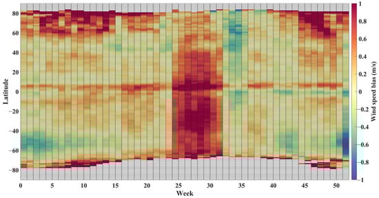
Figure 1.
Geographic distribution of the weekly mean difference between CSCAT and ECMWF wind speed.
A variety of long-term, consistent scatterometer wind datasets, namely climate data records (CDRs), have been developed in the past few years. For instance, the Ocean and Sea Ice Satellite Application Facility (OSI SAF) of the European Organisation for the Exploitation of Meteorological Satellites (EUMETSAT) released the reprocessed Seawinds, ERS, Oceansat2, and ASCAT-A CDR data, which together span the period from 1999 to 2014 [10]. Remote Sensing Systems recalibrated the L1B backscatter coefficient data of QuikSCAT and ASCAT and reprocessed the corresponding L2B winds utilizing a new geophysical model function (GMF) [11,12]. In addition, the Jet Propulsion Laboratory (JPL) improved the L2A and L2B processing algorithms for QuikSCAT and reprocessed the full data records from 1999 to 2009 [13]. Several new aspects differentiate the above activities from NRT wind processing. Firstly, the recalibration of sea surface σ0s is performed in order to eliminate the instability of scatterometer outputs during the entire mission period. Moreover, NWP-reanalyzed winds have been used instead of operational models’ outputs for ambiguity removal [10], and an improved wind GMF might be used to achieve more consistent wind retrievals than the NRT product [13].
So far, consistent scatterometer data records have not been extended to the period of CSCAT mission life. Regarding the important variations in CSCAT NRT winds informed by the meteorological users, it is necessary to investigate the potential instabilities of CSCAT instruments and to carry out a comprehensive calibration for its backscatter measurements. Afterward, the CSCAT L2B winds are reprocessed based on the recalibrated backscatter data in order to offer more precise and stable sea surface wind fields. This paper is organized as follows: Section 2 introduces the datasets and the methods used in this study. Section 3 addresses the potential reasons for the unstable performance of CSCAT measurements. The effectiveness of the proposed method is examined in Section 4 by analyzing the collocated CSCAT, ECMWF, and buoy data. Finally, Section 5 summarizes the main conclusions.
2. Data and Methods
2.1. Data
The main objective of this paper was to investigate the instability of CSCAT measurements and to develop an improved calibration procedure for the reprocessing campaign of CSCAT L2 data; thus, data from only one year (2021) of the CSCAT NRT products (version 3.3) were used in this study. All the CSCAT products are provided by the National Satellite Ocean Application Service (NSOAS). L1B data mainly consist of the raw σ0 values and observation geometries of high-resolution ground cells, namely slices in scatterometry [1]. Each slice is about 10 km along the range direction, and 11~15 km along the azimuthal direction, while L2 data mainly include the aggregated σ0s with a spatial resolution of 25 km × 25 km (L2A), and the retrieved wind vectors with a grid resolution of 25 km × 25 km as well (L2B). In this paper, the CSCAT 25 km L2 data (including L2A and L2B) were used to assess the temporal consistency of CSCAT winds, and L1B data were used to reprocess the L2 winds.
ECMWF forecast winds, rather than the reanalyzed winds, are used as a reference in the following sections. On the one hand, this model’s forecast winds are already included in the CSCAT L2B files, which may facilitate the development of the reprocessing software. On the other hand, ECMWF forecast winds have been proven effective in a variety of scatterometry studies, notably for calibration purposes [14]. Note that the ECMWF model provides forecast winds twice a day (00 and 12 h), so the forecast cycle, which is closer to the CSCAT observation time, is used by the processor. In practice, ECMWF winds are obtained by interpolating three ECMWF 3-hourly forecast winds, both spatially and temporally, to the CSCAT acquisition position and time [1].
In addition, CSCAT observations were collocated with the moored buoy data in order to verify the performance of the proposed method below. The number of moored buoys used in this paper was 96, including the National Data Buoy Center (NDBC) buoys off the coasts of North America, the Tropical Ocean–Atmosphere (TAO) buoy arrays, the Prediction and Research Moored Array (PIRATA) in the Atlantic, etc. For the sake of comparison, the buoy wind speed at a certain anemometer height was converted to 10 m equivalent-neutral winds using the Liu–Katsaros–Businger (LKB) model [15,16]. The temporal and spatial differences between CSCAT and buoy measurements were 30 min and 25 km, respectively. The total value of CSCAT–buoy collocations was about 82.5 k.
2.2. Methods
The absolute calibration of the scatterometer σ0s is essential for the retrieval of high-quality geophysical parameters, such as sea surface winds, sea ice, soil moisture, etc. For wind data assimilation, the global bias of scatterometer-derived wind speed should be less than 0.2 m/s, which requires a radiometric error of <0.2 dB. Following the system design of CSCAT [1], the σ0 value of a particular slice is estimated as follows:
where , , and are acquired by the signal channel, the external noise channel, and the internal calibration channel of the receiver, respectively. consists of the backscatter energy from Earth’s surface, as well as the thermal noise and the microwave radiation from the surface and atmosphere, while includes the thermal noise and the incident radiation of the antenna. C is a constant correction factor that accounts for the different gains/losses between the above two channels, and X is the radar calibration factor involving the antenna gain pattern, the measurement area, the distance from the satellite to the slice, the systematic gains and losses, etc. Ideally, both C and X should be calibrated in order to achieve a high quality of σ0 values. However, the estimation of C is not trivial, which requires not only the raw measurement data (L1A) but also the “true” instrument parameters, e.g., the gains or losses of those devices not shared by the above two receiver channels [17]. Consequently, the conventional calibration campaign mainly addresses the σ0 bias (i.e., Δσ0 in dB) induced by the potential errors associated with the X factor.
Due to the lack of knowledge of the “true” instrument parameters, in this study, we only calibrated the -factor-induced σ0 bias. A widely used NWP ocean calibration (NOC) technique, which is estimated to be with a precision of ~0.1 dB [18], was adopted to assess the calibration coefficients for CSCAT. First, the difference between the CSCAT σ0s and the simulated σ0s from the collocated ECMWF winds, together with the wind geophysical model function (GMF), was calculated [19]. Discrepancies between the above two sets of σ0s are mainly caused by the systematic errors in the knowledge of GMF and instrument parameters (e.g., antenna gain, system’s gains and losses, etc.), and the random errors in NWP winds and the measured σ0s. Second, the systematic errors, which are regarded as the calibration coefficients, were derived by averaging the difference between the measured and the simulated σ0s for given antenna incidence and/or azimuth angles [19]. The average processing eliminates the random errors in the discrepancies between the measured and the simulated σ0s.
More specifically, given the radar frequency, the relationship between the simulated backscatter and the wind field as well as the scatterometer antenna parameters can be expressed as follows:
Subsequently, the bias correction (i.e., the calibration coefficient) is derived from the weighted averaging of A0 over the wind speed domain. The overall NOC procedure for the numerical implementation is shown in Figure 2. Note that Equation (3) presumes that the wind direction distributes uniformly over 0~, so an inversed weighting is used in the calculation of the calibration coefficient for the ith wind speed bin (denoted as Δi), i.e.,
where the subscripts i and j denote the indices of the wind speed bin and relative wind direction bin, respectively. The weighting factor for a particular relative wind direction bin is proportional to the inverse value of the number of samples (Ni,j) within that bin. The mean measured σ0 and the simulated one for a given wind speed and direction bin are indicated by and , respectively.
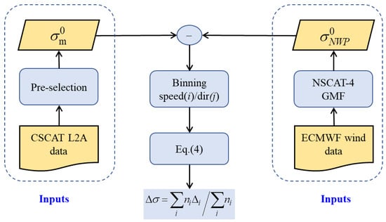
Figure 2.
Flowchart of the NWP ocean calibration. Ni,j and ni denote the number of samples of the corresponding wind speed/direction bin.
As shown in Figure 2, the preselection module filters out “poor-quality” data according to the quality control (QC) flag in L2B data and then segregates the dataset into different subsets according to the characteristics of CSCAT, e.g., polarization, incidence/azimuth angles, a certain period of the mission, etc. Similar to the prior scatterometer wind processing [20], the QC flag is developed based on the inversion residual of the maximum likelihood estimator (MLE) and is used to discern between good- and poor-quality winds, as well as the measured σ0s. The MLE is written as follows [21]:
where N is the number of views within a particular wind vector cell (WVC), is the observed backscatter coefficient, is the simulated backscatter coefficient using the NSCAT-4 GMF, and denotes the normalized measurement error. During the reprocessing campaign, MLE thresholds are simply adapted to reject a similar number of data as the prior pencil-beam scatterometers, such that the overall rejection ratio is about 6%.
The relevant aspects of this module and the data binning process are described as follows:
- (1)
- The quality control (QC)-accepted data and the observations in the latitudes between 60°S and 60°N were selected for further analysis;
- (2)
- The subsets were differentiated according to polarization and the incidence angle in bins of 1° for θ ∈ [28°, 51°];
- (3)
- In each incidence angle bin, the dataset was further separated into 64 categories according to the antenna azimuth in bins of 5.625°, in line with the onboard look-up table for the slice construction [1];
- (4)
- In each incidence–azimuth category, collocations were separated into certain groups following the ECMWF wind speed in bins of 1 m/s and the relative wind direction in bins of 10°, and the difference between the mean measured σ0s and the mean simulated σ0s (i.e., ) was calculated for each group.
Note that the MLE value changed with the calibrated σ0s, so an iterative approach (see Figure 3) was carried out to update the calibration coefficients until they converged. Finally, the L2 product of the last iteration was recorded as the reprocessed wind product.
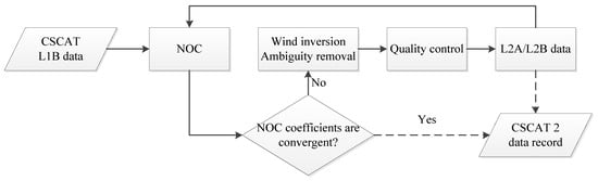
Figure 3.
The iterative procedure for the CSCAT wind reprocessing.
3. Overview of the CSCAT Stabilities
3.1. Ocean Calibration Coefficients Δσ0
In the operational L2 processing, only the X-factor-induced σ0 bias (see Equation (1)) was considered using the NOC. The ocean calibration coefficients were derived using one month of CSCAT observations (i.e., February 2021 for the NRT product version 3.3), and then were fixed in the L2 processor for wind inversion. Such implementation may lead to poor-quality wind retrieval (see Figure 1, weeks 25–33) in case the radar faced unexpected signal fluctuations. On the other hand, one may estimate the NOC coefficients periodically using a fixed-length running window, in order to reveal the potential signal distortions during CSCAT exploitation. To determine the window size for the periodical NOC, we considered the internal calibration signal, which is used to achieve accurate calibration of the transmit power and the receiver gain [18] and is illustrated in Figure 4. Normally, the internal calibration output is very stable, and the signal-to-noise ratio (SNR) of the internal calibration channel is generally larger than 40 dB [1]. However, Figure 4 shows that temporal variations with a fluctuation of up to 0.6 dB (~15%) persisted over the long term, which occurred in line with the abnormal period (weeks 25–33) in Figure 1. Ideally, it is recommended to estimate daily calibration coefficients precisely for every incidence angle, signal polarization, and antenna azimuth. Given the fact that the NOC requires a vast volume of data to reduce the estimation uncertainty, a window size of seven days (i.e., a weekly window) was used in this study.
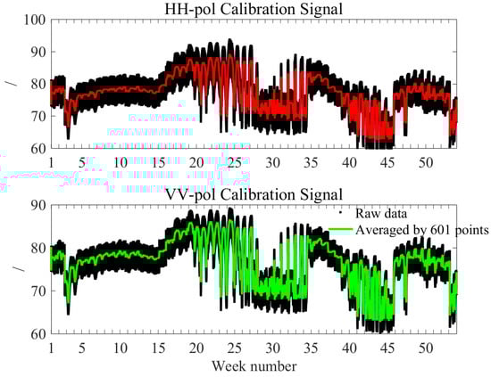
Figure 4.
Time series of the outputs (dimensionless digital numbers) of the internal calibration channel (Ec, see Equation (1)) in the year 2021. The red and green curves indicate the averaged digital numbers based on a 601-point running window.
For the stability evaluation, we primarily considered the relative temporal variation in the NOC coefficient for every incidence angle, which is expressed as follows:
where ti denotes the week number of the year 2021, and the reference week number tr can be set up arbitrarily (tr = 10 is used in the following section). As shown in Figure 5a, the normalized NOC coefficients (i.e., ) markedly varied around week 15, weeks 25–35, and week 43 for both vertical (V) and horizontal (H) polarization processes, implying that the signal level of CSCAT instrument experienced unexpected changes during those periods. During weeks 25–33, the normalized NOC coefficients of the HH beam were about ~1 dB lower than the reference week, leading to ~1 m/s of bias in the retrieved winds. The inconsistency among different incidence angles of the VV beam increased up to 0.5 dB from the 25th week. Moreover, Figure 5a shows that the temporal variation in HH-pol (lower panel) was generally more noticeable than that of VV-pol (upper panel), and the variation in the incidence angles that were close to the side lobes (low antenna gain) was also more prominent than those acquired in the main lobes (~40°). Since the latter cases (the VV beam and close to 40°) are generally of higher SNR than the former cases (the HH beam and close to side lobes), one may speculate that the signal-level fluctuation is more likely to occur under low SNR conditions.
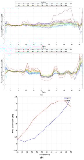
Figure 5.
(a) Temporal variation in the normalized NOC coefficients in 2021. The upper panel is for the VV beam, and the lower one is for the HH beam; (b) the 10th week’s NOC coefficients as a function of the incidence angle for VV (blue) and HH (red) beams, respectively.
3.2. Low SNR Measurements
Following the above speculation, the characteristics of low SNR measurements were specifically examined. As aforementioned, the observations at high incidence angles generally correspond to low SNR (see Figure 8a in [1]); hence, the acquisitions at > 48° are mainly studied in this section. First, the number of σ0s obtained at high incidence angles was evaluated using the CSCAT NRT data. Figure 6 shows the temporal evolution of the percentage of CSCAT σ0s acquired at > 48°. Although the variation is very small (<0.5%), the curve shows fairly good consistency with Figure 4. Note that only the QC-accepted data were used for the statistical analysis, so it could be inferred that the number of QC-accepted data at high incidence angles slowly increased from weeks 5 to 25 and then dramatically decreased around week 24. Following the relationship between the QC indicator (MLE) and the quality of σ0s used in wind inversion (see Equation (5)), one may further infer that low SNR observations at high incidence angles are of great significance to the stability of CSCAT-derived winds.
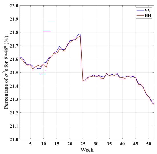
Figure 6.
Temporal variation relative to the percentage of CSCAT σ0s acquired at > 48°. Here, the percentage is defined as the number of σ0s for > 48° over the total number of σ0s.
The accuracy of scatterometer σ0s highly depends on the radar SNR. Lower SNR not only leads to poorer quality of σ0 estimation but also results in more negative σ0 values [22]. As shown in Equation (1), the noise contribution should be subtracted from the radar-measured power before the estimation of σ0; thus, a larger noise value is more likely to result in negative σ0. Theoretically, the ratio of negative σ0 values could be up to 50% at extremely low SNR conditions [22]. Figure 7 shows the percentage of negative σ0 s ( > 48° and < 2 m/s) as a function of the week number in 2021. Compared with the results of 2019 [1], it is clear that the number of negative σ0 values was overestimated (i.e., larger than the theoretical upper limit of 50%) for the VV beam, implying that the noise floor of the VV beam was overestimated in the L1 processing of CSCAT [17]. In contrast, the noise level of the HH beam was underestimated, notably around weeks 25–32, and week 37. Consequently, the problem of noise subtraction is the essential reason for the variation in σ0 quality.
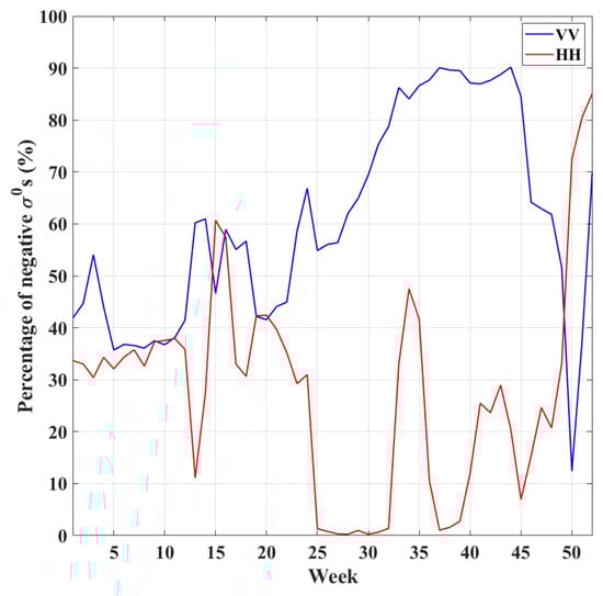
Figure 7.
Time variation relative to negative σ0 percentage at large incidence angles (larger than 48°) and low wind speed (smaller than 2 m/s) for VV (blue) and HH (red) beams, respectively.
3.3. Inversion Residual
In addition to σ0 stability, it is also relevant to evaluate the variation in the wind inversion residual (see Equation (5)), which directly reflects the quality of scatterometer-derived winds. Figure 8 illustrates the mean MLE value as a function of latitude (y-axis) and week number (x-axis) in 2021. As expected, it shows good consistency with the variations in the wind speed bias in Figure 1, as well as the temporal evolution of NOC coefficients in Figure 5a.
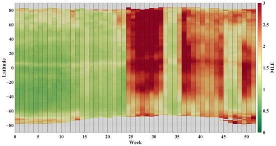
Figure 8.
Geographic distribution of the weekly mean MLE value.
Moreover, the inversion residual (MLE) was used to discern between good- and poor-quality winds in terms of quality control (QC). Similar to the operational σ0 calibration, the MLE QC threshold was derived using a certain month (i.e., February 2021) of CSCAT L2 data and then fixed in the processor for CSCAT wind QC. Therefore, the fluctuation in σ0 quality would result in larger MLE values and, in turn, lead to the rejection of more data through the operational QC procedure, as shown in Figure 9. In other words, the stability of scatterometer winds can be easily evaluated using the inversion residual, which will be further used in Section 4 to assess the consistency of the reprocessed winds.
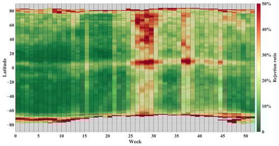
Figure 9.
Geographic distribution of the weekly mean QC rejection ratio.
4. Results
Ideally, the noise subtraction model in the L1 processor (Equation (1)), especially the noise correction factor C, should be redeveloped in order to accommodate the signal fluctuations caused by the changes in instrument characteristics, e.g., sensor temperature, system’s gains and losses, transmitted power, etc. However, this is not trivial due to the limited knowledge of the detailed monitoring results of each and every onboard component. Consequently, the alternative approach proposed in Section 2.2 was used to reprocess the CSCAT data, with the objective of achieving a more consistent wind data record than the operational outputs.
Instead of the values shown in Figure 5b, a series of two-dimensional NOC coefficients were implemented in practice during the reprocessing; that is, the weekly calibration factor is expressed as a function of the incidence angle and the antenna’s azimuth angle, as shown in Figure 10. Then, the calibrated radar backscatter coefficient is given by . Although the variation in Δσ0 along the azimuth angle is small, it clearly shows non-negligible asymmetry (>0.2 dB) at a given incidence angle for both VV and HH beams.
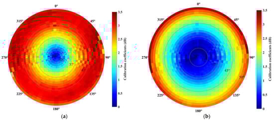
Figure 10.
Illustration of the 10th week’s CSCAT two-dimensional NOC coefficients (dB) for the HH beam (a) and VV (b) beams, respectively.
As stated before, the stability of scatterometer winds can be assessed through the temporal evolution of wind speed bias, the mean MLE value, as well as the QC rejection ratio. Therefore, the characteristics of Figure 1, Figure 8, and Figure 9 were re-evaluated, and the results are shown in Figure 11, Figure 12 and Figure 13, respectively. Although a large speed bias persists in high latitudes of the Northern Hemisphere (>60°N), these plots clearly demonstrate that the reprocessed data are generally of better temporal consistency than those of the NRT product. The persistent large speed bias (~1 m/s) in Figure 11 is probably due to the geophysical factors not accounted for by the wind GMF (e.g., sea ice, sea surface temperature (SST)), rather than the calibration procedure. Specifically, the positive bias during weeks 1–15 and 41–50 is likely caused by the sea-ice contamination not detected using the QC scheme, and the negative bias during weeks 25–32 is likely caused by the SST effects not accounted for by wind GMF [23]. The evaluation of sea-ice contamination and SST effects is beyond the scope of this paper.
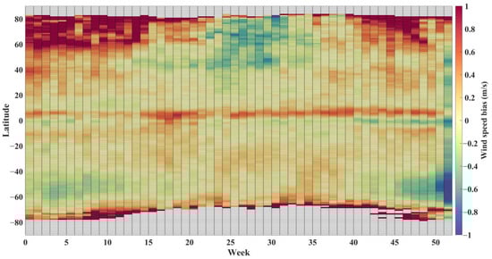
Figure 11.
Distribution of the CSCAT-reprocessed wind speed bias with respect to ECMWF.
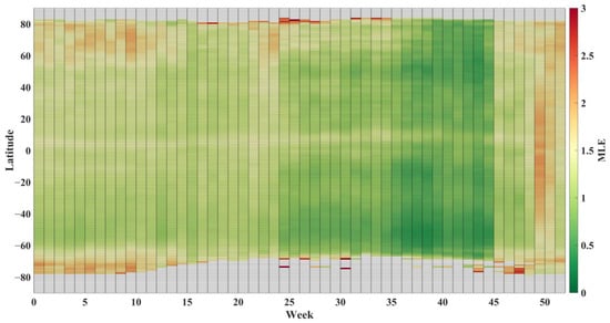
Figure 12.
Distribution of the CSCAT’s mean MLE for the reprocessed data.
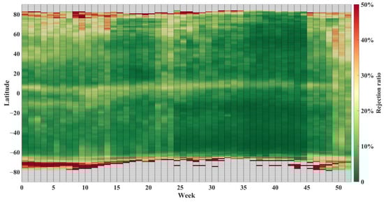
Figure 13.
Distribution of the QC rejection ratio for the reprocessed data.
More specifically, the wind quality during weeks 25–32 was estimated, and the results are shown in Figure 14. Both ECMWF (left panels) and buoy winds (right panels) were used as references. The upper panels illustrate the results of the NRT wind product, and the lower ones show those of the reprocessed winds. Relevant statistical scores, i.e., correlation coefficient (cc), speed bias, the standard deviation (SD) of the speed difference, and the number of QC-accepted data (QC rejection ratio), are shown in the upper-left corner of each panel. The NRT processing rejected more than a quarter of sea surface data, which was much more than the expectation (5~6%). Even so, the QC-accepted CSCAT winds were significantly biased with respect to both ECMWF and buoy references, while the proposed method significantly decreased both the speed bias and the rejection ratio, without a significant increase in the SD score. For the wind direction, the reprocessing did not markedly change the overall statistical scores (not shown), probably due to the fact that the removal of the two-dimensional variational ambiguity in combination with a multiple solution scheme (144 ambiguous solutions with a direction interval of 2.5°) already provided a spatial analysis of sea surface winds to effectively resolve the retrieved wind ambiguities.
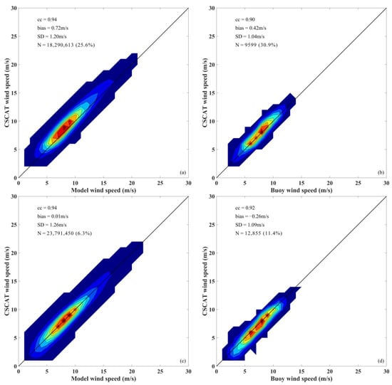
Figure 14.
CSCAT NRT winds versus ECMWF wind speed (a) and buoy wind speed (b). Images (c,d) are the same as (a,b) but for the reprocessed CSCAT wind speed. Only the observations during weeks 25–32 are evaluated.
5. Conclusions
CSCAT is a Ku-band rotating fan-beam scatterometer with a wide range of incidence angles (28–51°), which provides a new observation geometry with regard to prior scatterometers and presents unprecedented challenges for the calibration of radar backscatter coefficients. Since its launch, extensive efforts have been made in order to retrieve high-quality winds from CSCAT observations. Generally, CSCAT-derived winds were found to have good performance in terms of RMS errors. However, the wind speed bias showed significant variations with time as compared to the reference winds, either ECMWF forecasts or buoy measurements. Such variation became prominent since the failure of the onboard traveling wave tube amplifier (December 2019).
Therefore, this paper provides an overview of CSCAT stabilities in terms of calibration coefficients, low SNR measurements, and inversion residuals. It was found that the variation in calibration coefficients was more significant for lower SNR measurements. Further analysis revealed that the essential problem could be the noise subtraction procedure in L1 processing, which overestimated (underestimated) the noise floor for the VV (HH) beam, leading to poor-quality σ0 estimation and wind retrieval [24]. The variation in the noise level of CSCAT, however, is apparently caused by the noise correction factor C in Equation (1), which may drift with the onboard instrument temperature but is set to be a constant value in the NRT processor. As such, a more flexible and accurate estimation C is required. This needs to be further investigated together with the consideration of the sensor developer and the satellite manufacturer.
In terms of L2 processing, a simple running-window-based calibration was proposed for reprocessing the CSCAT wind data. In this process, the calibration coefficients were updated using the NOC method every week and then used in the wind retrieval. Since the instrument gain/loss may slightly vary with the antenna azimuth, in this study, the calibration factor was considered a function of both the incidence angle and the antenna’s azimuth angle. Compared with the NRT product, the reprocessed winds showed a significant reduction in wind speed bias during weeks 25–32, i.e., speed bias of ~1 m/s was reduced to <0.2 m/s. Moreover, the volume of QC-accepted reprocessed data was much more than the NRT product, without markedly degrading the statistical scores. Overall, the reprocessing improved the temporal stability of CSCAT winds and resulted in a more consistent wind data record than the NRT product.
Nonetheless, the proposed method is not able to accommodate the signal fluctuation which varies faster than the running window (one week) and thus is not feasible for NRT processing. Therefore, further studies are needed to improve the noise subtraction procedure in L1 processing and to develop a method that enables the fast calibration of the CSCAT measurements over the sea surface.
Author Contributions
Conceptualization, W.L.; methodology, X.M.; software and validation, W.L. and X.M.; formal analysis, W.L. and Y.H.; writing—review and editing, X.M. and W.L. All authors have read and agreed to the published version of the manuscript.
Funding
This research was supported by the National Key R&D Program of China(No. 2022YFC3104900/2022YFC3104902), and partly by the Graduate Student Practice and Innovation Program of Jiangsu Province (SJCX22_0374).
Data Availability Statement
Not applicable.
Acknowledgments
The authors would like to acknowledge NSOAS for straightforward and rapid access to the CSCAT data. We would also like to Risheng Yun from the National Space Science Center of the Chinese Academy of Sciences for providing Figure 4.
Conflicts of Interest
The authors declare no conflict of interest.
References
- Liu, J.; Lin, W.; Dong, X.; Lang, S.; Yun, R.; Zhu, D.; Zhang, K.; Sun, C.; Mu, B.; Ma, J.; et al. First results from the rotating fan beam scatterometer onboard CFOSAT. IEEE Trans. Geosci. Remote Sens. 2020, 58, 8793–8806. [Google Scholar] [CrossRef]
- Lin, W.; Dong, X. Design and optimization of a Ku-band rotating, range-gated fanbeam scatterometer. Int. J. Remote Sens. 2011, 32, 2151–2171. [Google Scholar] [CrossRef]
- Lin, W.; Dong, X.; Portabella, M.; Lang, S.; He, Y.; Yun, R.; Wang, Z.; Xu, X.; Zhu, D.; Liu, J. A perspective on the performance of the CFOSAT rotating fan-beam scatterometer. IEEE Trans. Geosci. Remote Sens. 2018, 57, 627–639. [Google Scholar] [CrossRef]
- Ye, H.; Li, J.; Li, B.; Liu, J.; Tang, D.; Chen, W.; Yang, H.; Zhou, F.; Zhang, R.; Wang, S. Evaluation of CFOSAT scatterometer wind data in global oceans. Remote Sens. 2021, 13, 1926. [Google Scholar] [CrossRef]
- Zhai, X.; Wang, Z.; Zheng, Z.; Xu, R.; Dou, F.; Xu, N.; Zhang, X. Sea Ice Monitoring with CFOSAT Scatterometer Measurements Using Random Forest Classifier. Remote Sens. 2021, 13, 4686. [Google Scholar] [CrossRef]
- Li, Z.; Verhoef, A.; Stoffelen, A. Bayesian sea ice detection algorithm for CFOSAT. Remote Sens. 2022, 14, 3569. [Google Scholar] [CrossRef]
- Chen, Y.; Cui, Y.; Lin, W.; Liu, J.; Sun, C.; Lang, S. The impacts of assimilating CFOSAT scatterometer winds for Typhoon cases based on real-time rain quality control. Atmos. Res. 2023, 285, 106621. [Google Scholar] [CrossRef]
- Xu, Y.; Liu, J.; Xie, L.; Sun, C.; Liu, J.; Li, J.; Xian, D. China-France Oceanography Satellite (CFOSAT) simultaneously observes the typhoon-induced wind and wave fields. Acta Oceanol. Sin. 2019, 38, 158–161. [Google Scholar] [CrossRef]
- Wu, W.; Du, Y.; Qian, Y.K.; Chen, J.; Jiang, X. Large South Equatorial Current meander in the southeastern tropical Indian Ocean captured by surface drifters deployed in 2019. Geophys. Res. Lett. 2022, 49, e2021GL095124. [Google Scholar] [CrossRef]
- Verhoef, A.; Vogelzang, J.; Verspeek, J.; Stoffelen, A. Long-term scatterometer wind climate data records. IEEE J. Sel. Top. Appl. Earth Obs. Remote Sens. 2017, 10, 2186–2194. [Google Scholar] [CrossRef]
- Ricciardulli, L. ASCAT on MetOp-A Data Product Update Notes. Remote Sens. Syst. Tech. Rep. 2016, 5, 40416. [Google Scholar]
- Ricciardulli, L.; Wentz, F.J. A scatterometer geophysical model function for climate-quality winds: QuikSCAT Ku-2011. J. Atmos. Ocean. Technol. 2015, 32, 1829–1846. [Google Scholar] [CrossRef]
- Fore, A.G.; Stiles, B.W.; Chau, A.H.; Williams, B.A.; Dunbar, R.S.; Rodríguez, E. Point-wise wind retrieval and ambiguity removal improvements for the QuikSCAT climatological data set. IEEE Trans. Geosci. Remote Sens. 2013, 52, 51–59. [Google Scholar] [CrossRef]
- Zhao, X.; Lin, W.; Portabella, M.; Wang, Z.; He, Y. Effects of rain on CFOSAT scatterometer measurements. Remote Sens. Environ. 2022, 274, 113015. [Google Scholar] [CrossRef]
- Bidlot, J.-R.; Holmes, D.J.; Wittmann, P.A.; Lalbeharry, R.; Chen, H.S. Intercomparison of the performance of operational ocean wave forecasting systems with buoy data. Weather Forecast 2002, 17, 287–310. [Google Scholar] [CrossRef]
- Liu, W.T.; Katsaros, K.B.; Businger, J.A. Bulk parameterization of air-sea exchanges of heat and water vapor including the molecular constraints at the interface. J. Atmos. Sci. 1979, 36, 1722–1735. [Google Scholar] [CrossRef]
- Yun, R.; Dong, X.; Liu, J.; Lin, W.; Zhu, D.; Ma, J.; Lang, S.; Wang, Z. CFOSAT Rotating Fan-Beam Scatterometer Backscatter Measurement Processing. Earth Space Sci. 2021, 8, e2021EA001969. [Google Scholar] [CrossRef]
- Stoffelen, A. A simple method for calibration of a scatterometer over the ocean. J. Atmos. Ocean. Technol. 1999, 16, 275–282. [Google Scholar] [CrossRef]
- Li, Z.; Stoffelen, A.; Verhoef, A.; Verspeek, J. NWP Ocean Calibration for the CFOSAT wind scatterometer and wind retrieval evaluation. Earth Space Sci. 2021, 8, e2020EA001606. [Google Scholar] [CrossRef]
- Portabella, M.; Stoffelen, A. Characterization of residual information for SeaWinds quality control. IEEE Trans. Geosci. Remote Sens. 2002, 40, 2747–2759. [Google Scholar] [CrossRef]
- Stoffelen, A.; Portabella, M. On Bayesian scatterometer wind inversion. IEEE Trans. Geosci. Remote Sens. 2006, 44, 1523–1533. [Google Scholar] [CrossRef]
- Plant, W.J. Effects of wind variability on scatterometry at low wind speeds. J. Geophys. Res. 2000, 105, 16899–16910. [Google Scholar] [CrossRef]
- Wang, Z.; Stoffelen, A.; Fois, F.; Verhoef, A.; Zhao, C.; Lin, M.; Chen, G. SST dependence of Ku-and C-band backscatter measurements. IEEE J. Sel. Top. Appl. Earth Obs. Remote Sens. 2017, 10, 2135–2146. [Google Scholar] [CrossRef]
- Zhang, K.; Dong, X.; Zhu, D.; Yun, R.; Wang, B.; Yu, M. An improved method of noise subtraction for the CFOSAT scatterometer. IEEE J. Sel. Top. Appl. Earth Obs. Remote Sens. 2021, 14, 7506–7515. [Google Scholar] [CrossRef]


Disclaimer/Publisher’s Note: The statements, opinions and data contained in all publications are solely those of the individual author(s) and contributor(s) and not of MDPI and/or the editor(s). MDPI and/or the editor(s) disclaim responsibility for any injury to people or property resulting from any ideas, methods, instructions or products referred to in the content. |
© 2023 by the authors. Licensee MDPI, Basel, Switzerland. This article is an open access article distributed under the terms and conditions of the Creative Commons Attribution (CC BY) license (https://creativecommons.org/licenses/by/4.0/).