Article

Estimation of Anthocyanins in Leaves of Trees with Apple Mosaic Disease Based on Hyperspectral Data

College of Nature Resources and Environment, Northwest A&F University, Yangling 712100, China
*
Author to whom correspondence should be addressed.
Remote Sens. 2023, 15(7), 1732; https://doi.org/10.3390/rs15071732
Submission received: 6 February 2023 / Revised: 17 March 2023 / Accepted: 21 March 2023 / Published: 23 March 2023
(This article belongs to the Special Issue Crop Disease Detection Using Remote Sensing Image Analysis II)

Abstract

:
Anthocyanins are severity indicators for apple mosaic disease and can be used to monitor tree health. However, most of the current studies have focused on healthy leaves, and few studies have estimated the anthocyanin content in diseased leaves. In this study, we obtained the hyperspectral data of apple leaves with mosaic disease, analyzed the spectral characteristics of leaves with different degrees of Mosaic disease, constructed and screened the spectral index sensitive to anthocyanin content, and improved the estimation model. To improve the conciseness of the model, we integrated Variable Importance in Projection (VIP), Partial Least Squares Regression (PLSR), and Akaike Information Criterion (AIC) to select the optimal PLSR model and its independent variables. Sparrow Search Algorithm-Random Forest (SSA-RF) was used to improve accuracy. Results showed the following: (1) anthocyanin content increased gradually with the aggravation of disease. The reflectance of the blade spectrum in the visible band increased, the red edge moved to short wave, and the phenomenon of “blue shift of spectrum” occurred. (2) The VIP-PLSR-AIC selected 17 independent variables from 21 spectral indices. (3) Variables were used to construct PLSR, Back Propagation (BP), Support Vector Machine (SVM), Random Forest (RF), and SSA-RF to estimate anthocyanin content. Results showed the estimation accuracy and stability of the SSA-RF model were better than other models. The model set determination coefficient ( R 2 ) was up to 0.955, which is 0.047 higher than that of the RF model and 0.138 higher than that of the SVM model with the lowest accuracy. The model was constructed at the leaf scale and can provide a reference for other scale studies, including a theoretical basis for large-area, high-efficiency, high-precision anthocyanin estimation and monitoring of apple mosaics using remote sensing technology.

Graphical Abstract

1. Introduction

Apple mosaic disease [1] is a viral disease that affects most orchards. Severe infections will affect leaf photosynthesis and cause early deciduous development, resulting in yield reduction. Timely identification of the degree of disease in fruit trees is of great significance for maintaining the economic interests of fruit farmers. Anthocyanin (Anth) [2] is one of the three main pigments in plant tissues, and changes in its content can reflect the physiological conditions of plants [3]. Therefore, the estimation of anthocyanin content in apple leaves [4] can be used to monitor the disease status.
Hyperspectral technology [5,6,7,8] has become widely used in plant biochemical parameter monitoring because of its characteristics of high resolution, high efficiency, lack of damage [9], and real-time observations, providing an effective means [10] for the implementation of fine agriculture. Estimation of biochemical parameters is an important method for monitoring vegetation growth [11,12,13], and research in this area is relatively mature. Gu used hyperspectral data to estimate the content of anthocyanins in maize leaves to grasp the growth status of maize [14]. Hernandez judged the ripening of grapes by estimating the anthocyanin content of grapes [15]. Yang used hyperspectral data to generate a visualization of the changes in anthocyanin content of litchi during storage [16]. Researchers have studied and constructed various vegetation indices [17,18,19,20], for example, the Difference Spectral Index (DSI), Ratio Spectral Index (RSI), and Normalized Difference Spectral Index (NDSI). Lopes modified DSI, RSI, and NDVI; combined linear, exponential, power, and logarithmic regression in the modeling process; and confirmed the feasibility of using the spectral index to estimate carotenoid and anthocyanin content in lettuce [21]. Some scholars have found that the vegetation index constructed after first- and second-order differential transformation of the original spectrum [22,23,24,25] can improve the accuracy of biochemical parameter content estimation. Wumuti used the multi-dimensional spectral index to build estimation models of wheat leaf area, and the spectral index after first-order differential treatment performed best [26]. Moreover, some scholars have constructed a vegetation index for anthocyanin estimation by selecting sensitive bands in the visible and near-infrared bands. These include the Red/Green index (RG), Anthocyanin Content Index (ACI), and Modified Anthocyanin Content Index (MACI) [27,28]. Feng used ACI to build a CNN model and successfully distinguished infected cabbage from healthy cabbage [29]. When plant species or health status change, the composition and content of anthocyanins in leaves change, so the adaptability and robustness of the existing spectral indices need to be further verified.
Since 2010, the application of machine learning in parameter inversion research has gradually increased [30,31,32,33,34]. Compared with traditional population optimization algorithms that are prone to fall into local optimal solutions and slow convergence rate, the Sparrow Search Algorithm (SSA), which was created in 2020, has shown improved ability to solve problems [35]. The Sparrow Search Algorithm is widely used in image recognition and element concentration prediction [36,37,38]. Minxi [39] used SSA to improve Random Forest (RF), which reduced the parameter optimization time and improved the accuracy of the molecular prediction model of drug compounds antagonizing the activity of the ER α gene. Chang [40] detected a distributed radar target with SSA-RF and concluded that it had higher detection performance than other classical methods. Additionally, Liu [41] used Grey Wolf Algorithm-Support Vector Machines (GWO-SVM), GWO-RF, SSA-SVM, and SSA-RF models to predict and assess the availability of groundwater, and the results showed that the prediction accuracy of the SSA-RF model was the highest (0.764). In summary, the improvement method of the RF model using SSA has been widely used in many fields, but it is rarely used in crop parameter estimation, and most studies do not consider conciseness of the estimation model, where the least independent variables are used to obtain the best estimation accuracy.
When vegetation is under disease stress, anthocyanin concentration will change obviously, and the variation rules of anthocyanin concentration caused by different diseases are different. Therefore, the estimation of anthocyanin content in apple leaves can be used to monitor the incidence of apple Mosaic disease. However, most existing studies focused on healthy leaves, and there needed to be more research on the variation of anthocyanin concentration in diseased leaves. Therefore, this study focused on apple leaves suffering from mosaic disease. The samples in this study included leaves with different disease degrees, aiming to explore the changes of anthocyanin concentration and spectral characteristics of leaves throughout the whole period. Further, using hyperspectral data, a machine learning method that can accurately estimate the concentration of anthocyanins was obtained. This model can monitor the anthocyanin content through remote sensing technology, and farmers can find and treat fruit trees in time at the early stage of disease.
To address these problems, we undertook the following studies: (1) Analysis of the spectral characteristics of apple mosaic disease, and study of the variation in anthocyanin content in affected leaves; (2) The correlation with anthocyanin content was used as the criterion to select the spectral index for model construction; (3) Variable importance in projection (VIP) was introduced, and then a partial least squares regression (PLSR) was used to establish anthocyanin content estimation models with different numbers of variables. The Akaike Information Criterion (AIC) was used to obtain the optimal independent variable, and this optimal independent variable was used as the anthocyanin estimation model parameters. This can improve the estimation accuracy, while ensuring the conciseness of the model; (4) A Random Forest model based on the Sparrow Search Algorithm (SSA-RF) was used. To ensure the advantages of the RF model, such as fast operation speed, strong anti-interference ability, and strong anti-overfitting ability, the SSA model was used to iteratively optimize the parameters of the RF model in order to enhance the stability of the model.

2. Materials and Methods

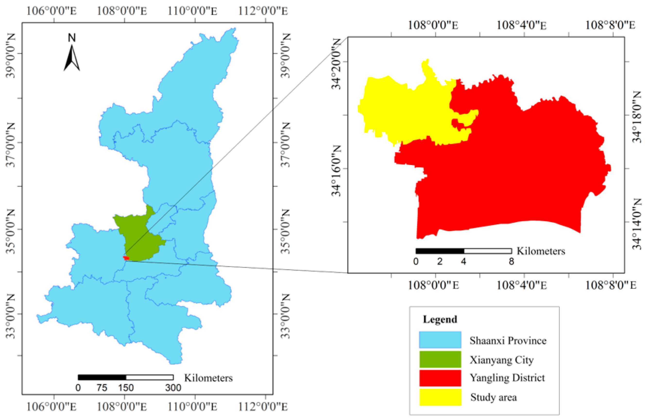
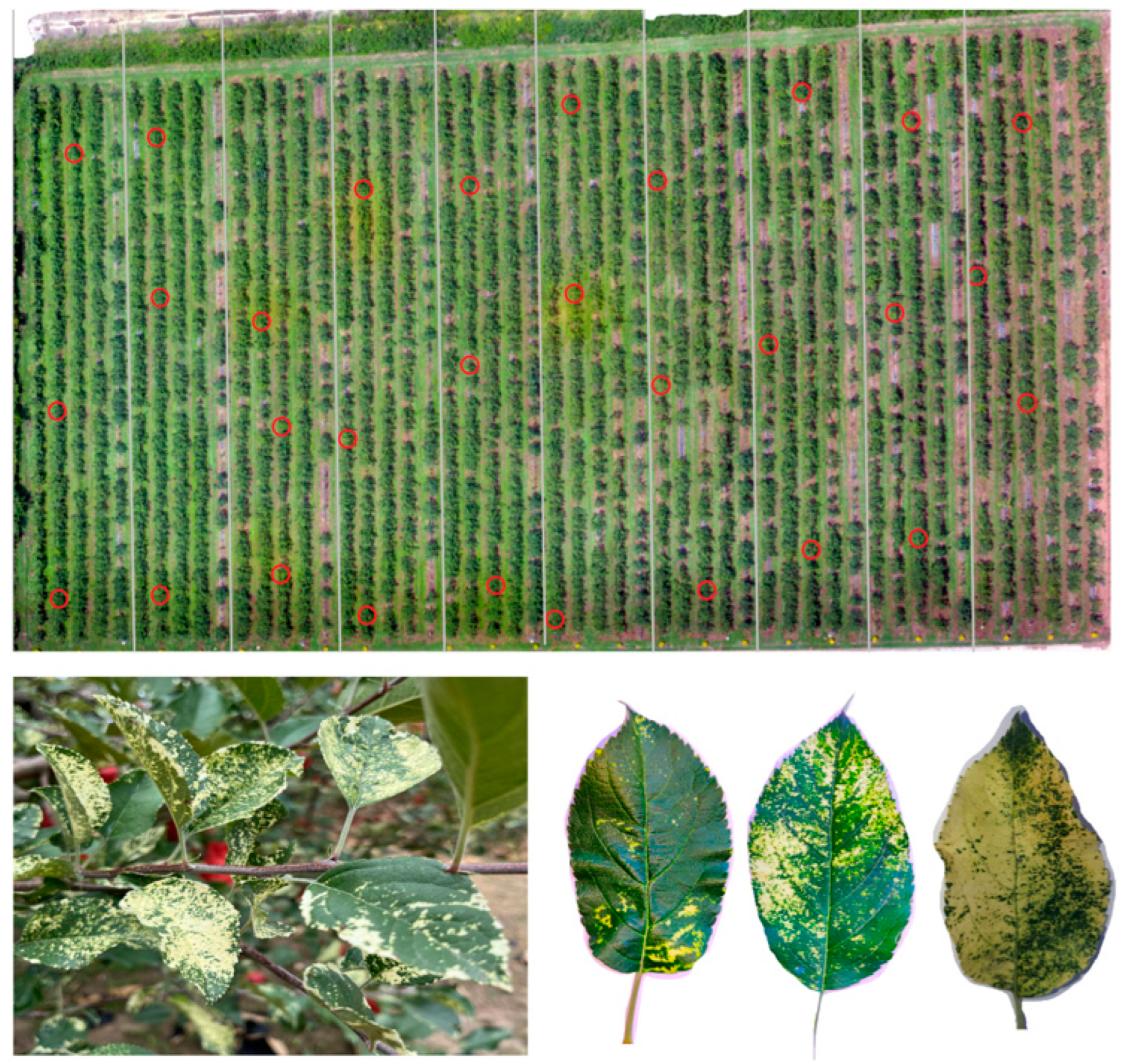
2.1. Study Area Overview and Experimental Design

The study area was located in Yangling District, Xianyang City, Shaanxi Province of China (108°0′57″, 34°18′47″), Weihe Plain, with relatively flat land and fertile soil. It is a continental monsoon climate area with an average annual temperature of 12.9 °C and average annual precipitation of 635.1 mm. This area is suitable for apple planting and has a long history of this practice; therefore, it was selected as the experimental area for research (Figure 1).
The apple trees were all 10 years old in the test area. Thirty trees infected with Mosaic disease were selected for sampling during the peak disease period (June 19). The study collected 12 leaves from each tree (Figure 2), and 360 leaves were collected. The collected leaf samples were stored in sealed plastic bags, placed in a fresh-keeping box with ice cubes, and quickly brought back to the laboratory to obtain the anthocyanin content and hyperspectral data.

2.2. Data Acquisition and Preprocessing

Dualex 4 (FORCE-A, Orsay, France) was used to determine the anthocyanin content of the apple leaves, which was used as its true value for subsequent study. Each leaf was measured three times at different positions, and the average value was taken as the leaf anthocyanin content [42,43].
In the laboratory, an SVC HR-1024i (Spectra Vista Crop, Poughkeepsie, NY, USA) and its companion vegetation-specific reflectance probe was used for spectral analysis. The SVC probe had a built-in lighting source and a special transformer to maintain light and voltage stability. The spectral detection range was 350–2500 nm. Before the spectral measurement, the instrument was calibrated. After the correction curve was stable, the apple leaf was placed in the blade clamp of the probe for measurement. Multiple reflectance curves of anthocyanin position were measured, the average value was taken as the final spectral reflectance curve of the leaf, and 360 hyperspectral data were obtained.
Anthocyanins are mainly related to near-infrared, short-wave, and visible bands; therefore [28], spectral reflectance in the range of 400–1000 nm was selected for this study. The spectra were resampled at 1 nm intervals, and a Savitzky–Golay filter [44] was used for noise reduction. The processed spectral data were used as original spectra for the first- and second-order differential transformations, and the first- and second-order differential spectrum were obtained, respectively.
The data were sorted according to the severity of disease from light to severe using stratified sampling, with 4/5 as the modeling set and 1/5 as the verification set.

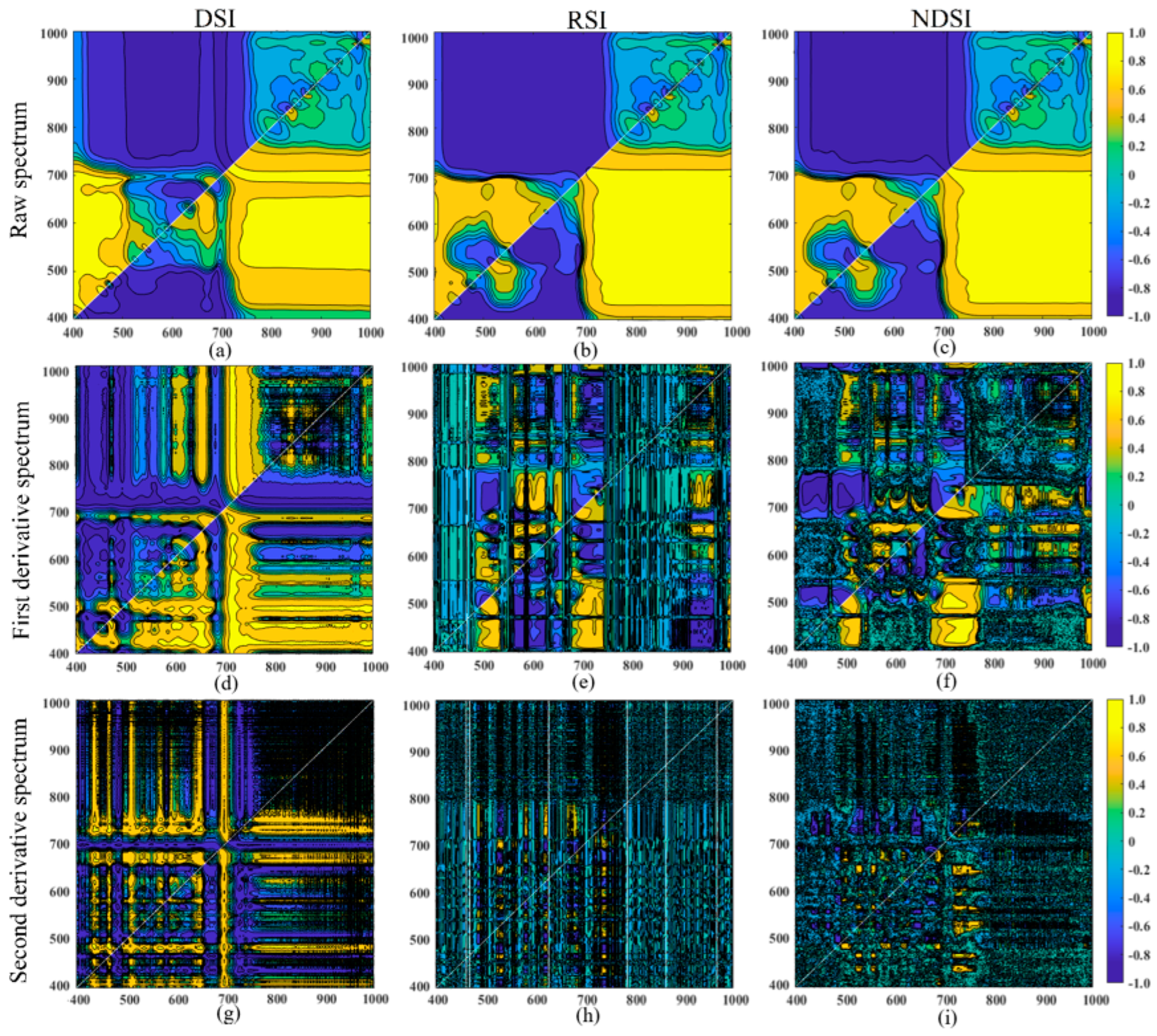
2.3. Construct the Sensitivity Spectral Index of Anthocyanins

Under the influence of mosaic disease, the internal structure and pigment content of apple leaves changed greatly, and the spectral characteristics also changed. Trilateral parameters are variables based on spectral position characteristics, which can better reflect changes in spectral characteristics and anthocyanin content. Roy [45] used the red-edge spectral index to detect nutrient elements lacking in vegetation and the change in chlorophyll content and demonstrated that the red-edge spectral index was significantly correlated with chlorophyll content and could effectively monitor the change in chlorophyll content. Therefore, this study not only selected a variety of common spectral indices but also selected six trilateral parameters in order to build the model.
The research of Zhang [46] showed that the creation of a spectral index based on spectral data after differential transformation is conducive to improving estimation accuracy. Therefore, any pairwise combination operation is performed on the full bands of the original spectrum, the first-order differential spectrum, and the second-order differential spectrum to construct three spectral indices, DSI, RSI, and NDSI, to determine the optimal band combination for estimating the anthocyanin content.
The 21 spectral indices obtained for this study are shown in Table 1.

2.4. Modeling Method

2.4.1. Variable Importance in Projection (VIP)

Variable projection importance [52] is a method of variable screening based on PLSR. It calculates the explanatory ability of independent variables relative to dependent variables and screens independent variables according to this result [53]. The formula is as follows:
V I P j = K h = 1 m ( r 2 ( y , C h ) W h j 2 ) h = 1 m r 2 ( y , C h )
where K is the number of independent variables, m is the number of components extracted from the original independent variable, C h is the principal component extracted from the relevant independent variable, and r ( y , C h ) is the correlation coefficient between the dependent variable and principal component and represents the explanatory ability of the principal component to anthocyanin content (y). W h j 2 is the weight of the independent variable in the principal component. The higher the value of V I P j , the stronger the interpretation ability of the anthocyanin content [54].

2.4.2. Akaike Information Criterion (AIC)

The Akaike Information Criterion [55] is a standard for measuring the goodness of the statistical model fit, which can measure the complexity of the estimated model and the goodness of the fitted data. For the PLSR model, the AIC can be expressed as:
AIC = n l n S p 2 + 2 K
where n is the number of leaves, S p 2 is the sum of the squares of the model, and K is the number of independent variables in the model.

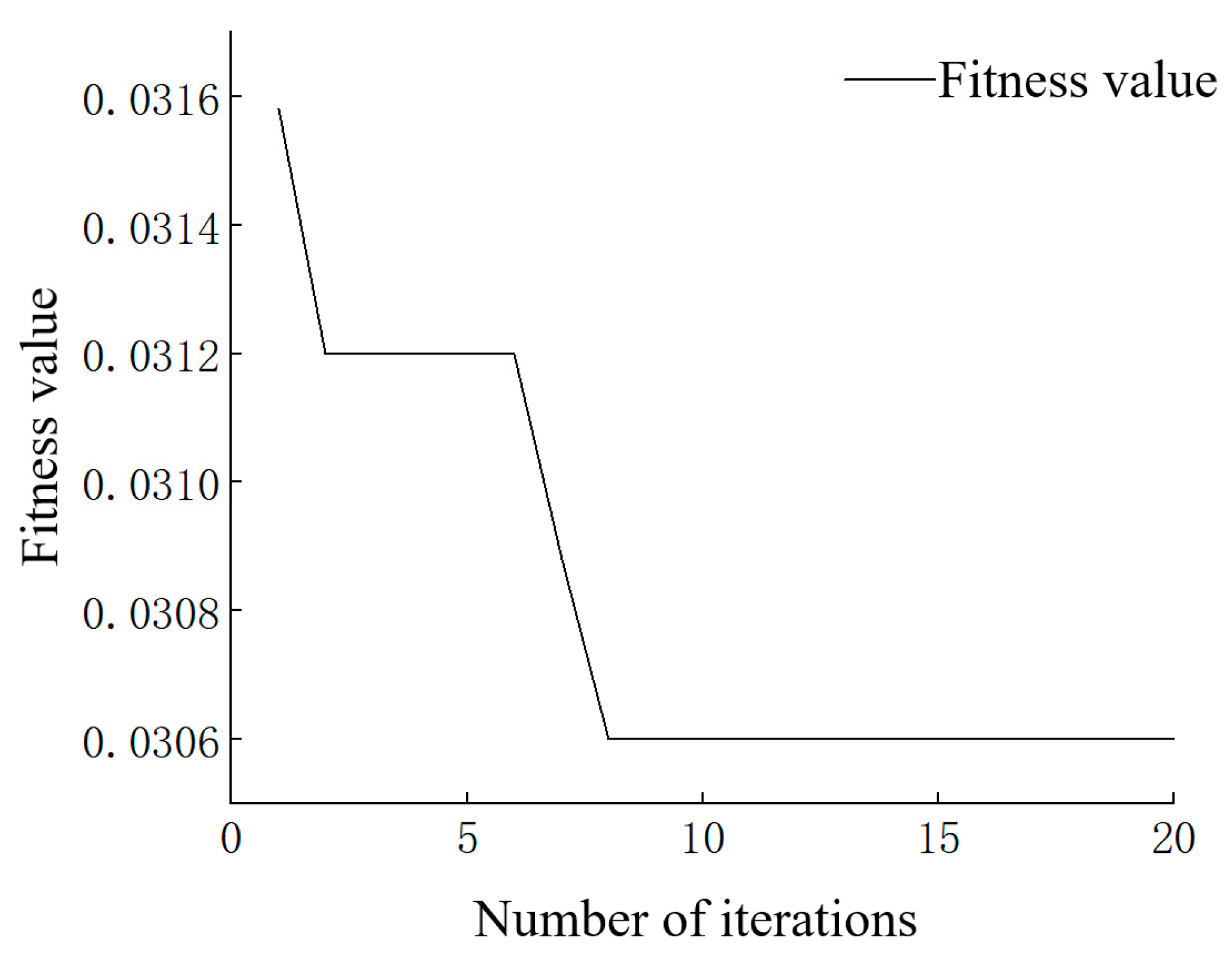
2.4.3. Sparrow Search Algorithm-Random Forest (SSA-RF)

Random Forest (RF) algorithm [56] is a classification regression model that combines multiple decision trees whose output is determined by individual trees. RF does not require distribution assumptions regarding response covariate relationships, and the process uses average decision trees to make statistically reliable estimates to reduce the risk of overfitting. However, this algorithm also has some disadvantages because of the randomness of the RF itself and the fact that the prediction results fluctuate.
The Sparrow Search Algorithm (SSA) [57] has strong optimization ability and fast convergence. The main idea is to conduct local and global searches by imitating the foraging and anti-predation behaviors of sparrows. The sparrow foraging process is the process of algorithm optimization. The SSA comprises discoverers, entrants, and scouts. The discoverer usually has a high fitness value and is responsible for providing foraging areas and directions to the entrant. To obtain better food, the entrant will closely follow the discoverer, monitor, and obtain food at the same time, to ensure their predation rate. When the scouts find the predator, they immediately send an alarm signal, and all sparrows respond with anti-predator behavior.
The position of sparrows can be represented as:
X = [ x 1 , 1 x 1 , 2 x 1 , d x 2 , 1 x 2 , 2 x 2 , d x n , 1 x n , 2 x n , d ]
where n is the number of sparrows and d is the dimension of the variable to be optimized. Then, the fitness values of all sparrows can be expressed as:
F X = [ f = ( [ x 1 , 1   x 1 , d ] ) f = ( [ x 2 , 1   x 2 , d ] ) f = ( [ x n , 1   x n , d ] ) ]
where the value of each row in FX represents the fitness value of the individual. Moreover, the discoverer’s position update formula is as follows:
X i , j ( t + 1 ) = { X i , j ( t ) · e x p ( i α · T ) , R < S T X i , j ( t ) + Q · L , R S T
where t is the current number of iterations, T is the maximum number of iterations, Xi,j(t) represents the value of the jth dimension of the ith sparrow at iteration t, α is a random number of [0, 1], R(R [0, 1]) is the warning value, ST(ST [0.5, 1]) is the safety value, Q is a random number subject to the normal distribution, and L represents a matrix of 1 × d, where each element is 1. When R < ST, there is no predator around, and the discoverer can conduct a large-scale search; When RST, the scout will immediately send out an alarm signal when finding the predator, and all sparrows will quickly fly to other safe areas.
The entrant’s position update formula is as follows:
X i , j ( t + 1 ) = { Q · e x p ( X w o r s t ( t ) X i , j ( t ) i 2 ) , i > n 2 X p ( t + 1 ) + | X i , j ( t ) X p ( t + 1 ) | · A + · L , i n 2
Xp(t + 1) is the position with the best fitness value among the current discoverers, xworst(t) is the position with the worst global fitness, A+ = AT(AAT)−1, A represents a column vector with the same dimension as the sparrow individual, and the internal elements are randomly composed of 1 and −1. When i     n 2 , the entrants will actively follow the discoverer to move towards a better feeding position; When i > n 2 , the entrants will use the exp function to get rid of the current poor foraging position.
The scout’s position update formula is as follows:
X i , j ( t + 1 ) = { X i , j ( t ) + C · ( | X i , j ( t ) X w o r s t ( t ) | f i f w + ε ) , f i = f g X b e s t ( t ) + β · | X i , j ( t ) X b e s t ( t ) | , f i > f g
Xbest(t) is the current global optimal location and β is a step-size control parameter. C [−1, 1] is a random number and fi is the fitness value of the current sparrow individual. fg and fw are the current global best and worst fitness values, respectively. ε is a smaller constant to avoid zero in the denominator. When fi > fg, the sparrow is at the edge of the population and vulnerable to predators. When fi = fg, the sparrow in the middle of the population is aware of the danger, so it needs to be close to other sparrows to reduce the probability of being prey.
The RF is mainly affected by the number of minimum leaf nodes and the number of decision trees. Therefore, SSA was used to optimize the two parameters of the RF, which can improve the stability and accuracy of the model [58]. The optimization process is as follows:
(1)
Set initialization population, iteration number, predator ratio, and warning value.
(2)
The RF model is established according to the initial population, and the fitness is calculated and ranked.
(3)
SSA updates the location of predators, scouts, and entrants.
(4)
Feedback the results to the RF model, calculate the fitness, and update the position of the sparrow.
(5)
Judge whether the best fitness is obtained. If so, exit SSA and output RF results. Otherwise, repeat steps (2) to (4).

3. Results

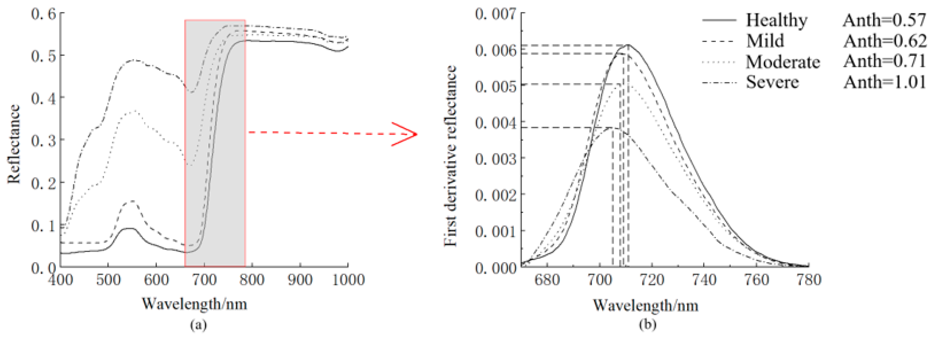
3.1. Spectral Characteristics of Mosaic Leaves

The symptoms of mosaic disease are yellow spots on the leaves, and with the aggravation of the disease, the affected area increases while the leaves gradually turn white. It was found that the spectral characteristics of diseased apple leaves also changed owing to changes in the cell structure. With the aggravation of the disease, the concentration of anthocyanin in leaves increases and the content of chlorophyll decreases, leading to the weakening of photosynthetic capacity and absorption of red and blue light. The reflectance at 400–680 nm increases significantly [59], especially the reflection peak near the wavelength of 554 nm, as shown in Figure 3a.
Trilateral parameters, such as spectral indices, commonly used to describe spectral characteristics, also differ considerably. The spectral red edge [60] is a plant-specific spectral feature formed by the strong absorption of light in the red band and the strong reflection of the near-infrared band of plant leaves. The spectral characteristics of the red edge of plants are usually identified by the position of the red edge, amplitude of the red edge, and area of the red edge, ranging from 680 nm to 760 nm. When plant leaves are damaged by diseases, the red-edge characteristics of the spectrum also change. As shown in Figure 3b, compared with the normal site, the area and amplitude of the red edge of the affected site decreased with aggravation of the disease, and the position of the red edge moved significantly in the shortwave direction [61]. There has been a “blue shift.”
The correlation between anthocyanin content and reflectance of the original spectrum, first differential spectrum, and the second differential spectrum was analyzed. The results are shown in Figure 4. Anthocyanin content was positively correlated with the original spectrum (Figure 4a) at 400–750 nm, and the correlation coefficient reached its maximum at 698 nm under red light (r = 0.846). The reflectance of most bands in the range of 400–1000 nm in the first- and second-order differential spectra (Figure 4b,c) was significantly correlated with the anthocyanin content. Janik [62] and Huang [63] estimated anthocyanin content using the near-infrared spectrum and obtained good results. It can be seen that both visible and near infrared bands are sensitive areas for anthocyanin content. To find the mathematical relationship between spectral data and anthocyanin content is the key to establishing the anthocyanin content estimation model using hyperspectral data. The correlation coefficient can help us find the right mathematical relationship. Therefore, when constructing the hyperspectral inversion model of anthocyanins, full spectral bands of different spectral transformations can be considered.

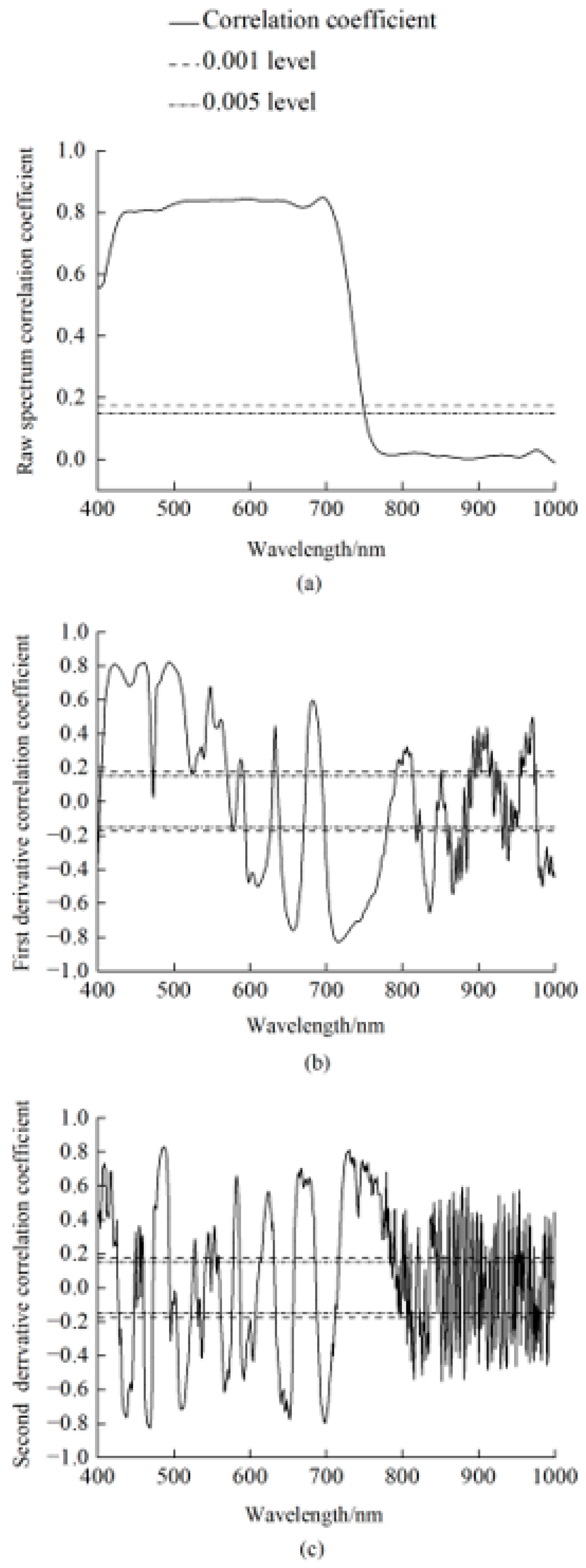
3.2. Correlation Analysis of the Spectral Index and the Anthocyanin Content

This study constructed the DSI, RSI, and NDSI of the original spectrum, and the first- and second-order differential spectra. As shown in Figure 5, the three spectral indices were significantly correlated with anthocyanin content (r > 0.8). The DSI of the three spectral datasets was significantly correlated with anthocyanins in the whole band (Figure 5a,d,g). RSI and NDSI were significantly correlated with anthocyanins at 680–1000 nm in the original spectrum (Figure 5b,c) and at 450–780 nm in the first- and second-order differential spectra (Figure 5e,f,h,i). As shown in Table 2, the bands of the nine spectral indices were concentrated at 400–800 nm, and the correlation between them and anthocyanins was greater than 0.8, which could be used to construct an anthocyanin estimation model.

3.3. Selection of the Spectral Index Independent Variables Based on the VIP-PLSR-AIC Method

3.3.1. VIP Analysis of Spectral Index and Anthocyanin Content

The results of the VIP analysis of the 21 spectral indices and anthocyanin contents are shown in Table 3. It can be seen from the table that among the 21 spectral indices, the largest VIP value is NDSI2 (VIP = 1.118) and the smallest is Sy (VIP = 0.219). In general, all spectral indices had strong explanatory abilities for anthocyanin content, with the DSI, RSI, and NDSI of the three spectral data having the strongest explanatory abilities, and VIP being greater than 1. The interpretative ability of the trilateral parameters was weak, and only the VIP value of Sr was greater than 1. According to a study by Dr. Wold [64], because the spectral index with a VIP value less than 0.8 contributes little to anthocyanin content, Dy and Sy are deleted. The VIP values of the remaining 19 spectral indices, from large to small, are: NDSI2, DSI2, NDSI1, RSI0, DSI0, DSI1, ACI, NDSI0, RSI2, RSI1, SPVI, CI3, Sr, CI4, MACI, Dr, Sb, RG, Db. Therefore, according to this sequence, spectral indices were successively increased as independent variables to conduct PLSR modeling analysis.

3.3.2. Selection of Optimal Independent Variables

According to the VIP value, the spectral index was successively increased as an input variable to conduct the PLSR modeling analysis for the modeling set. The optimal PLSR model and optimal independent variables were selected according to the AIC criterion. The results are presented in Table 4. The AIC value also changes when the number of independent variables changes. According to the principle of AIC [65], the model with the lowest AIC value in a set of models is the best to interpret data and contains the least number of free parameters, which are the optimal independent variables. As can be seen from the table, when the number of model independent variables in PLSR is 17, the AIC value reaches a minimum value (AIC = 59.632). Therefore, the PLSR model with 17 independent variables was selected as the optimal PLSR model, and its independent variables were the optimal independent variables.
y p = 0.30 x 1 + 0.11 x 2 + 0.56 x 3 + 4.50 x 4 0.49 x 5 0.09 x 6 3.66 x 7 2.18 x 8 + 0.26 x 9 0.13 x 10 2.71 x 11 + 0.90 x 12 + 2.71 x 13 0.69 x 14 + 0.24 x 15 0.54 x 16 + 1.02 x 17
where y p is the estimated anthocyanin content and xi is the spectral index ranking i in the VIP value.

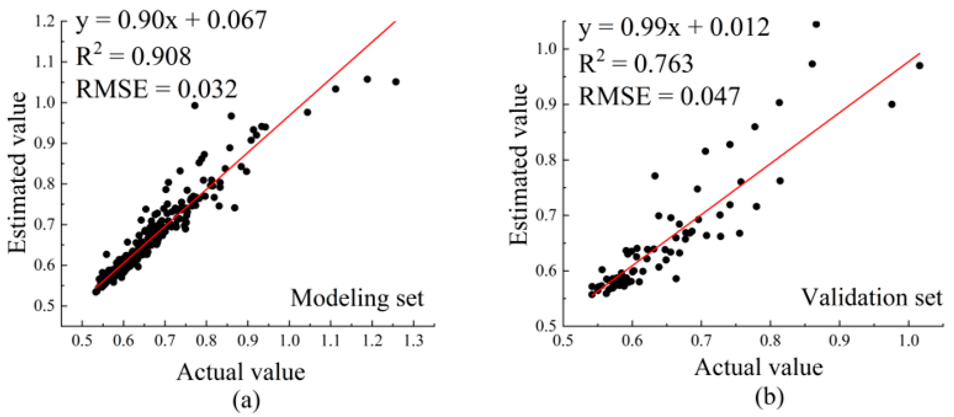
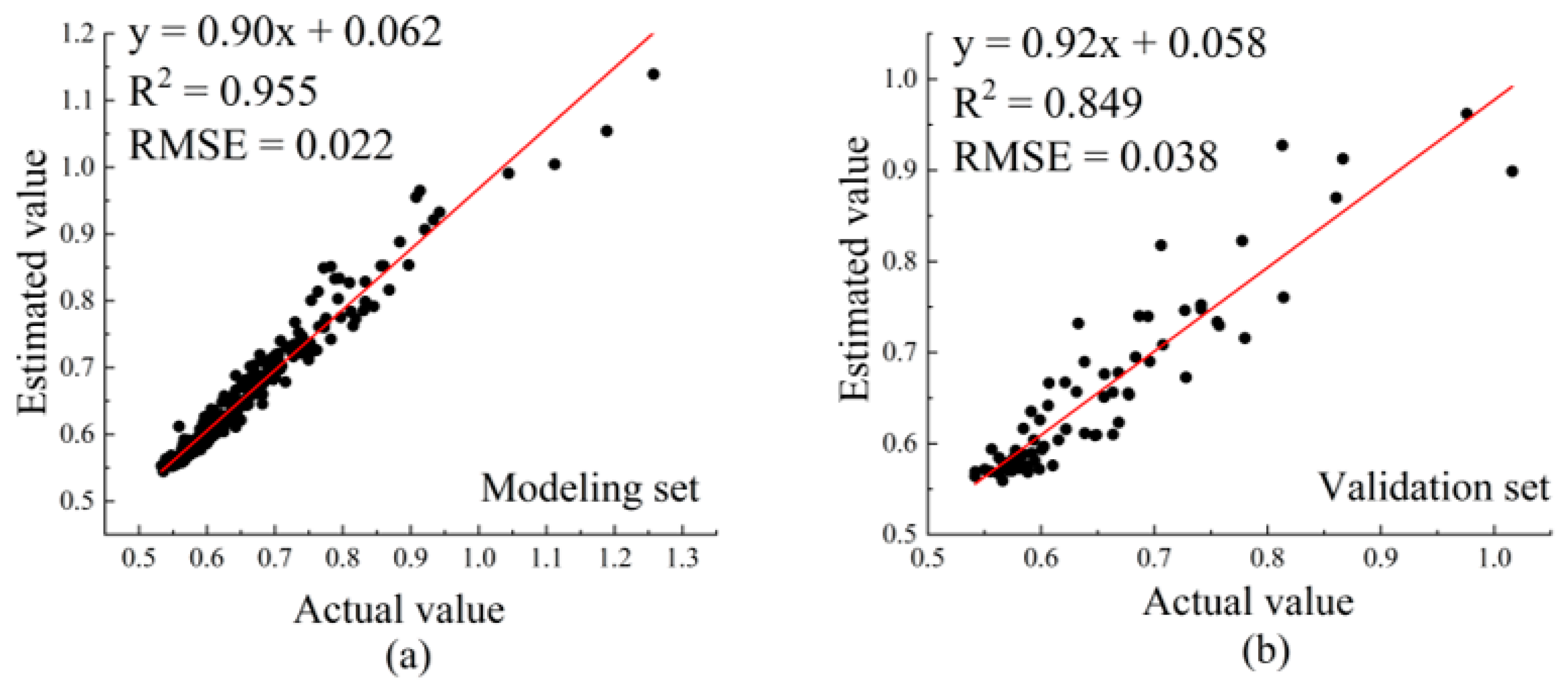
3.3.3. Establishment and Comparison of Hyperspectral Estimation Models for Anthocyanin Content in Apple Leaves

Seventeen optimal independent variables were used to establish RF and SSA-RF models to estimate the anthocyanin content. The number of decision trees and leaf nodes of the RF model were set to 5. The initial parameters of SSA were set as follows: population number 50, discoverer ratio 0.3, warning value 0.8, and maximum number of iterations, 20. The running results are shown in Figure 6. After the 8th iteration, the optimal fitness is 0.0306, the number of optimal decision trees was 20, and the minimum leaf node was 10. The estimated results for anthocyanin content are shown in Figure 7 and Figure 8, and both the modeling and verification sets achieved good estimated results. The Root Mean Square Error (RMSE) and Determination Coefficient ( R 2 ) were selected as evaluation indices to compare the estimation results. The RMES of the SSA-RF model in the modeling and validation sets were 0.022 and 0.038, and the R 2 values were 0.955 and 0.849, respectively. Compared to the RF model before improvement, the RMSE value of the modeling set was reduced by 31.25%, and the R 2 value increased by 5.18%. The RMSE value of the validation set decreased by 19.15%, and the R 2 value increased by 11.27%.
To determine the superiority of the SSA-RF model more directly, the BP and SVM models were added to estimate anthocyanin content. Through repeated training and testing of the model, the BP model parameters were determined as follows: learning rate, 0.001; the time step, 1; hidden size, 6; and iteration epoch, 500. The kernel function of the SVM model was RBF, penalty coefficient C was 0.66, and Gamma was 0.03. Comparing the estimated results of anthocyanin content in the PLSR, BP, SVM, RF, and SSA-RF models, it could be seen (Table 5) that for the anthocyanin content estimation results of the modeling dataset, the SVM model had the worst estimation ability (RMES = 0.056, R 2 = 0.717). In the validation set, the BP model exhibited the worst estimation ability (RMES = 0.049, R 2 = 0.743). In both the modeling and validation sets, the SSA-RF model was the best in terms of estimation accuracy and goodness of fit.

4. Discussion

4.1. Effect of Apple Mosaic Disease on Leaf Spectral Reflectivity and Anthocyanin Content

The measurement of pigment content in plants can be used to monitor their growth in real time, which is particularly useful for vegetation monitoring. Gao [66] explored spectral responses at different growth stages, providing a model for chlorophyll content estimation to meet the requirements of high-throughput phenotypic analysis. Pigment content can also reflect the environmental stress in vegetation. Ruyan [67] established a chlorophyll content estimation model using the wavelet coefficient features extracted from the smoothed spectra (WSMH1 and WSMH2) processed by the Mexican hat wavelet function to determine the stress of stripe rust in wheat. In addition, environmental stress at different growth stages has different effects on the pigment content. Chi [68] found that under ozone stress, wheat reduced chlorophyll content at different growth stages, especially at the filling stage. Existing studies mostly use chlorophyll, which is a common component in all leaves. Anthocyanins are the third major pigment in plant leaves and are a common component in all leaves. Anthocyanins can repair the light environment of leaves, and have the potential to regulate photosynthesis, limit photoinhibition and photobleaching, and defend against light damage [69]. Anthocyanins also have antioxidant effects, contributing to the repair of damaged leaves [70]. Therefore, dynamic monitoring of anthocyanin content can assist in understanding the physiological responses and resistance of vegetation, so as to judge to the degree of environmental stress.
The spectral characteristics of the hyperspectral data of healthy leaves and mosaic leaves were different in the visible band. With the aggravation of the disease, the reflectance of the leaves in the visible band gradually increased, and the position of the red edge moved to the short wave, resulting in a “blue shift” phenomenon. At the same time, anthocyanin content also increased, and the spectral reflectance of the leaves was significantly correlated with anthocyanin content. In conclusion, it is feasible to use hyperspectral data to estimate anthocyanin content to monitor the disease status of apple trees.

4.2. VIP-PLSR-AIC Method Selected the Optimal Argument Variables of the Model

In this study, 21 spectral indices were initially selected, concentrated in the visible band of 400–800 nm. The spectral reflectance of leaves with different degrees of disease in this band was significantly different, and the correlation between spectral indices and anthocyanin content was higher than 0.8, which met the research requirements. In this study, Dy and Sy, which were weak in explaining anthocyanin content, were excluded by the VIP analysis to ensure the accuracy of the model estimation results. Simultaneously, the AIC criterion was used to analyze the PLSR model, and RG and Db were deleted to obtain 17 optimal independent variables for modeling, ensuring the conciseness of the model. The estimation accuracy of the optimal independent variable modeling using VIP-PLSR-AIC screening was lowest in the SVM model (modeling set, RMES = 0.056, R 2 = 0.717) and highest in the SSA-RF model (modeling set, RMES = 0.022, R 2 = 0.955). The results show that the VIP-PLSR-AIC method can effectively ensure the estimation accuracy and conciseness of the model.

4.3. Evaluation of the SSA-RF Model

Traditional methods of measuring anthocyanin content in leaves are restricted by space, time, and other factors. However, machine learning methods combined with hyperspectral remote sensing technology can obtain anthocyanin content in leaves over a large area, at high speed, and with no damage. In this study, various machine learning methods, such as PLSR, BP, SVM, RF, and SSA-RF, were used to estimate the anthocyanin content. The accuracy of the estimation results varied significantly; however, all were satisfactory. The results showed that the best accuracy of anthocyanin content estimation in both the modelling and validation sets was the SSA-RF model, the worst accuracy of anthocyanin content estimation in the modeling set was the SVM model, and the worst accuracy of anthocyanin content estimation in the validation set was the BP model. Among them, SSA-RF is an algorithm optimized by the Sparrow Search Algorithm for Random Forests. Chen [71] used the SSA-RF algorithm to predict heavy metal content in soil. The results show that SSA can quickly find the optimal parameters of RF, and the accuracy of the prediction results is better than that of the other models. In this study, the SSA-RF model was superior to other estimation moduli in all aspects, and compared with the unimproved RF model, the model stability and accuracy were greatly improved. Therefore, the SSA-RF model was the optimal anthocyanin content estimation model in this study. The incidence area of mosaic disease is a single leaf, and it is difficult to obtain accurate data of the incidence area in large-scale images owing to low spectral resolution; therefore, this study was focused at the leaf scale. To solve this problem, Bhagyashree [72] used the Universal Pattern Decomposition Method (UPDM) to conduct the spectral reconstruction of Sentinel-2 data and obtain an AVIRIS-NG image. The applicability of the method for estimating chlorophyll was further verified using ground measurement data, which showed a good correlation value (r = 0.65). The results showed that the simulated AVIRIS-NG is very useful and can be used for vegetation parameter inversion. In future studies, spectral reconstruction of satellite remote sensing images can be carried out, and real-time monitoring of large orchards can be achieved using the independent variable selection method and anthocyanin estimation model in this study to provide help for the prevention and control of apple mosaic disease.

5. Conclusions

When apple trees suffer from mosaic disease, due to the change of cell structure, photosynthesis is weakened and anthocyanin content will increase with the increase in the disease degree; at the same time, the spectral characteristics of leaves also change. Therefore, a method of estimating anthocyanin content using leaf hyperspectral data was proposed to monitor the disease status of fruit trees. In this study, the proposed VIP-PLSR-AIC method screened the optimal argument variables for modeling, ensuring the conciseness of the model. Simultaneously, the Sparrow Search Algorithm was used to improve the Random Forest algorithm, and the SSA-RF model with higher estimation accuracy and more stability was obtained. The R 2 values of the modeling and verification sets of the sample estimation results were as high as 0.955 and 0.849, respectively. In conclusion, the VIP-PLSR-AIC method combined with the SSA-RF model can achieve a higher anthocyanin content estimation and effectively monitor the disease situation of apple trees.
In this study, the estimation of anthocyanin concentration in apples was based on the relationship between the variation of anthocyanin concentration caused by mosaic disease and the change of spectral characteristics. The changes in vegetation characteristics caused by different diseases varied. This method can be used to estimate the biochemical parameters of vegetation theoretically; however, the changes of biochemical parameters and spectral characteristics of vegetation must be determined first. Because of the different changes in biochemical parameters and spectral characteristics, the estimation model proposed in this study cannot guarantee good estimation accuracy. However, the research method can be used as the basis to obtain accurate estimation methods for the biochemical parameters of different diseased leaves.

Author Contributions

Conceptualization, Z.Z. (Zijuan Zhang); methodology, Z.Z. (Zijuan Zhang), D.J. and Z.Z. (Zhikang Zheng); software, Z.Z. (Zijuan Zhang), D.J. and Z.Z. (Zhikang Zheng); validation, Z.Z. (Zijuan Zhang), Z.Z. (Zhikang Zheng) and X.F.; formal analysis, Z.Z. (Zijuan Zhang) and D.J.; investigation, X.F.; resources, Z.Z. (Zijuan Zhang); data curation, K.L.; writing—original draft preparation, Z.Z. (Zijuan Zhang); writing—review and editing, Z.Z. (Zijuan Zhang) and D.J.; visualization, H.M.; supervision, Q.C.; project administration, Q.C.; funding acquisition, Q.C. All authors have read and agreed to the published version of the manuscript.

Funding

This research was funded by the National High Technology Research and Development Program of China (863 Program), grant number 2013AA102401-2.

Data Availability Statement

Data sharing is not application to this article.

Conflicts of Interest

The authors declare no conflict of interest.

References

  1. Grimova, L.; Winkowska, L.; Konrady, M.; Rysanek, P. Apple mosaic virus. Phytopathol. Mediterr. 2016, 55, 1–19. [Google Scholar] [CrossRef]
  2. Landi, M.; Tattini, M.; Gould, K.S. Multiple functional roles of anthocyanins in plant-environment interactions. Environ. Exp. Bot. 2015, 119, 4–17. [Google Scholar] [CrossRef]
  3. Lo Piccolo, E.; Landi, M.; Massai, R.; Remorini, D.; Guidi, L. Girled-induced anthocyanin accumulation in red-leafed Prunus cerasifera: Effect on photosynthesis, photoprotection and sugar metabolism. Plant Sci. 2020, 294, 110456. [Google Scholar] [CrossRef]
  4. Janeeshma, E.; Rajan, V.K.; Puthur, J.T. Spectral variations associated with anthocyanin accumulation; an apt tool to evaluate zinc stress in Zea mays L. Chem. Ecol. 2021, 37, 32–49. [Google Scholar] [CrossRef]
  5. Skoneczny, H.; Kubiak, K.; Spiralski, M.; Kotlarz, J. Fire Blight Disease Detection for Apple Trees: Hyperspectral Analysis of Healthy, Infected and Dry Leaves. Remote Sens. 2020, 12, 2101. [Google Scholar] [CrossRef]
  6. Fernandes, A.M.; Oliveira, P.; Moura, J.P.; Oliveira, A.A.; Falco, V.; Correia, M.J.; Melo-Pinto, P. Determination of anthocyanin concentration in whole grape skins using hyperspectral imaging and adaptive boosting neural networks. J Food Eng. 2011, 105, 216–226. [Google Scholar] [CrossRef]
  7. Ye, W.X.; Xu, W.; Yan, T.Y.; Yan, J.K.; Gao, P.; Zhang, C. Application of Near-Infrared Spectroscopy and Hyperspectral Imaging Combined with Machine Learning Algorithms for Quality Inspection of Grape: A Review. Foods 2023, 12, 132. [Google Scholar] [CrossRef]
  8. Ding, Y.; Zhao, X.F.; Zhang, Z.L.; Cai, W.; Yang, N.J.; Zhan, Y. Semi-Supervised Locality Preserving Dense Graph Neural Network With ARMA Filters and Context-Aware Learning for Hyperspectral Image Classification. IEEE Trans. Geosci. Remote Sens. 2022, 60, 12. [Google Scholar] [CrossRef]
  9. Gitelson, A.A.; Keydan, G.P.; Merzlyak, M.N. Three-band model for noninvasive estimation of chlorophyll, carotenoids, and anthocyanin contents in higher plant leaves. Geophys. Res. Lett. 2006, 33, 5. [Google Scholar] [CrossRef] [Green Version]
  10. Huang, J.F.; Wei, C.; Zhang, Y.; Blackburn, G.A.; Wang, X.Z.; Wei, C.W.; Wang, J. Meta-Analysis of the Detection of Plant Pigment Concentrations Using Hyperspectral Remotely Sensed Data. PLoS ONE 2015, 10, e0137029. [Google Scholar] [CrossRef] [Green Version]
  11. Wang, X.X.; Cai, G.S.; Lu, X.P.; Yang, Z.N.; Zhang, X.J.; Zhang, Q.G. Inversion of Wheat Leaf Area Index by Multivariate Red-Edge Spectral Vegetation Index. Sustainability 2022, 14, 15875. [Google Scholar] [CrossRef]
  12. Wu, B.; Zheng, H.; Xu, Z.L.; Wu, Z.W.; Zhao, Y.D. Forest Burned Area Detection Using a Novel Spectral Index Based on Multi-Objective Optimization. Forests 2022, 13, 1787. [Google Scholar] [CrossRef]
  13. Li, D.; Chen, J.M.; Yu, W.G.; Zheng, H.B.; Yao, X.; Cao, W.X.; Wei, D.D.; Xiao, C.C.; Zhu, Y.; Cheng, T. Assessing a soil-removed semi-empirical model for estimating leaf chlorophyll content. Remote Sens. Environ. 2022, 282, 113284. [Google Scholar] [CrossRef]
  14. Gu, X.H.; Cai, W.Q.; Fan, Y.B.; Ma, Y.; Zhao, X.Y.; Zhang, C. Estimating foliar anthocyanin content of purple corn via hyperspectral model. Food Sci. Nutr. 2018, 6, 572–578. [Google Scholar] [CrossRef] [Green Version]
  15. Hernandez-Hierro, J.M.; Nogales-Bueno, J.; Rodriguez-Pulido, F.J.; Heredia, F.J. Feasibility Study on the Use of Near-Infrared Hyperspectral Imaging for the Screening of Anthocyanins in Intact Grapes during Ripening. J. Agric. Food Chem. 2013, 61, 9804–9809. [Google Scholar] [CrossRef]
  16. Yang, Y.C.; Sun, D.W.; Pu, H.B.; Wang, N.N.; Zhu, Z.W. Rapid detection of anthocyanin content in lychee pericarp during storage using hyperspectral imaging coupled with model fusion. Postharvest Biol. Technol. 2015, 103, 55–65. [Google Scholar] [CrossRef]
  17. Tran, T.V.; Reef, R.; Zhu, X. A Review of Spectral Indices for Mangrove Remote Sensing. Remote Sens. 2022, 14, 4868. [Google Scholar] [CrossRef]
  18. Anchal, S.; Bahuguna, S.; Priti; Pal, P.K.; Kumar, D.; Murthy, P.V.S.; Kumar, A. Non-destructive method of biomass and nitrogen (N) level estimation in Stevia rebaudiana using various multispectral indices. Geocarto Int. 2022, 37, 6409–6421. [Google Scholar] [CrossRef]
  19. Mlynarczyk, A.; Konatowska, M.; Krolewicz, S.; Rutkowski, P.; Piekarczyk, J.; Kowalewski, W. Spectral Indices as a Tool to Assess the Moisture Status of Forest Habitats. Remote Sens. 2022, 14, 4267. [Google Scholar] [CrossRef]
  20. Psiroukis, V.; Darra, N.; Kasimati, A.; Trojacek, P.; Hasanli, G.; Fountas, S. Development of a Multi-Scale Tomato Yield Prediction Model in Azerbaijan Using Spectral Indices from Sentinel-2 Imagery. Remote Sens. 2022, 14, 4202. [Google Scholar] [CrossRef]
  21. Lopes, D.D.; Moura, L.D.; Neto, A.J.S.; Ferraz, L.D.L.; Carlos, L.D.; Martins, L.M. Spectral Indices for Non-destructive Determination of Lettuce Pigments. Food Anal. Method. 2017, 10, 2807–2814. [Google Scholar] [CrossRef]
  22. Tian, X.; Wen, B.W.; Qing, B.Z.; Yong, Z. Comparison of hyperspectral remote sensing inversion methods for leaf area index in winter wheat. Trans. Chin. Soc. Agric. Eng. 2013, 29, 139–147. [Google Scholar]
  23. Xia, J.; Teng, Z.; Qin, Z.; Ju, M.Y.; Ying, Y.D. Construction of remote sensing monitoring model of wheat stripe rust based on fractional differential spectral index. Trans. Chin. Soc. Agric. Eng. 2021, 37, 142–151. [Google Scholar]
  24. Bhadra, S.; Sagan, V.; Maimaitijiang, M.; Maimaitiyiming, M.; Newcomb, M.; Shakoor, N.; Mockler, T.C. Quantifying Leaf Chlorophyll Concentration of Sorghum from Hyperspectral Data Using Derivative Calculus and Machine Learning. Remote Sens. 2020, 12, 2082. [Google Scholar] [CrossRef]
  25. Li, C.C.; Wang, Y.L.; Ma, C.Y.; Ding, F.; Li, Y.C.; Chen, W.A.; Li, J.B.; Xiao, Z. Hyperspectral Estimation of Winter Wheat Leaf Area Index Based on Continuous Wavelet Transform and Fractional Order Differentiation. Sensors 2021, 21, 8497. [Google Scholar] [CrossRef] [PubMed]
  26. Wumuti, A.; Nijiati, K.; Chen, C.; Sawut, M. Estimation of Winter Wheat LAI Based on Multi-dimensional Hyperspectral Vegetation Indices. Trans. Chin. Soc. Agric. Mach. 2022, 53, 181–190. [Google Scholar]
  27. Ritchie, G.L.; Sullivan, D.G.; Vencill, W.K.; Bednarz, C.W.; Hook, J.E. Sensitivities of Normalized Difference Vegetation Index and a Green/Red Ratio Index to Cotton Ground Cover Fraction. Crop Sci. 2010, 50, 1000–1010. [Google Scholar] [CrossRef]
  28. Gitelson, A.A.; Chivkunova, O.B.; Merzlyak, M.N. Nondestructive estimation of anthocyanins and chlorophylls in anthocyanic leaves. Am. J. Bot. 2009, 96, 1861–1868. [Google Scholar] [CrossRef] [Green Version]
  29. Feng, L.; Wu, B.H.; Chen, S.S.; Zhang, C.; He, Y. Application of visible/near-infrared hyperspectral imaging with convolutional neural networks to phenotype aboveground parts to detect cabbage Plasmodiophora brassicae (clubroot). Infrared Phys. Technol. 2022, 121, 14. [Google Scholar] [CrossRef]
  30. Verrelst, J.; Camps-Valls, G.; Munoz-Mari, J.; Rivera, J.P.; Veroustraete, F.; Clevers, J.; Moreno, J. Optical remote sensing and the retrieval of terrestrial vegetation bio-geophysical properties—A review. ISPRS J. Photogramm. Remote Sens. 2015, 108, 273–290. [Google Scholar] [CrossRef]
  31. Garcia-Berna, J.A.; Ouhbi, S.; Benmouna, B.; Garcia-Mateos, G.; Fernandez-Aleman, J.L.; Molina-Martinez, J.M. Systematic Mapping Study on Remote Sensing in Agriculture. Appl. Sci. 2020, 10, 3456. [Google Scholar] [CrossRef]
  32. Le, T.H.; Liu, C.; Yao, B.; Natraj, V.; Yung, Y.L. Application of machine learning to hyperspectral radiative transfer simulations. J. Quant. Spectrosc. Radiat. Transf. 2020, 246, 106928. [Google Scholar] [CrossRef]
  33. Ding, Y.; Zhang, Z.L.; Zhao, X.F.; Hong, D.F.; Li, W.; Cai, W.; Zhan, Y. AF2GNN: Graph convolution with adaptive filters and aggregator fusion for hyperspectral image classification. Inf. Sci. 2022, 602, 201–219. [Google Scholar] [CrossRef]
  34. Ding, Y.; Zhang, Z.L.; Zhao, X.F.; Cai, W.; Yang, N.J.; Hu, H.J.; Huang, X.X.; Cao, Y.; Cai, W.W. Unsupervised Self-Correlated Learning Smoothy Enhanced Locality Preserving Graph Convolution Embedding Clustering for Hyperspectral Images. IEEE Trans. Geosci. Remote Sens. 2022, 60, 16. [Google Scholar] [CrossRef]
  35. Sun, C.J.; Gao, F. Remote Sensing Image Recognition Based on LOG-T-SSA-LSSVM and AE-ELM Network. Comput. Intell. Neurosci. 2022, 2022, 8077563. [Google Scholar] [CrossRef]
  36. Balaha, H.M.; Hassan, A.E.S. Skin cancer diagnosis based on deep transfer learning and sparrow search algorithm. Neural Comput. Appl. 2023, 35, 815–853. [Google Scholar] [CrossRef]
  37. Liu, J.; Hu, P.; Xue, H.; Pan, X.; Chen, C. Prediction of milk protein content based on improved sparrow search algorithm and optimized back propagation neural network. Spectrosc. Lett. 2022, 55, 229–239. [Google Scholar] [CrossRef]
  38. Yamaguchi, T.; Tanaka, Y.; Imachi, Y.; Yamashita, M.; Katsura, K. Feasibility of Combining Deep Learning and RGB Images Obtained by Unmanned Aerial Vehicle for Leaf Area Index Estimation in Rice. Remote Sens. 2021, 13, 84. [Google Scholar] [CrossRef]
  39. Rong, M.X.; Li, Y.; Guo, X.L.; Zong, T.; Ma, Z.Y.; Li, P.L. An ISSA-RF Algorithm for Prediction Model of Drug Compound Molecules Antagonizing ER? Gene Activity. Oncologie 2022, 24, 309–327. [Google Scholar] [CrossRef]
  40. Chang, J.Y.; Fu, X.J.; Zhao, C.X.; Lang, P.; Feng, C. Distributed Radar Target Detection Based on RF-SSA in Non-Gaussian Noise. Electronics 2022, 11, 2319. [Google Scholar] [CrossRef]
  41. Liu, R.; Li, G.L.; Wei, L.S.; Xu, Y.; Gou, X.J.; Luo, S.B.; Yang, X. Spatial prediction of groundwater potentiality using machine learning methods with Grey Wolf and Sparrow Search Algorithms. J. Hydrol. 2022, 610, 127977. [Google Scholar] [CrossRef]
  42. Cerovic, Z.G.; Masdoumier, G.; Ben Ghozlen, N.; Latouche, G. A new optical leaf-clip meter for simultaneous non-destructive assessment of leaf chlorophyll and epidermal flavonoids. Physiol. Plant. 2012, 146, 251–260. [Google Scholar] [CrossRef] [PubMed]
  43. Goulas, Y.; Cerovic, Z.G.; Cartelat, A.; Moya, I. Dualex: A new instrument for field measurements of epidermal ultraviolet absorbance by chlorophyll fluorescence. Appl. Optics 2004, 43, 4488–4496. [Google Scholar] [CrossRef] [PubMed]
  44. Yang, H.Y.; Yu, H.Y.; Liu, X.; Zhang, L.; Sui, Y.Y. Diagnosis of Cucumber Diseases and Insect Pests by Fluorescence Spectroscopy Technology Based on PCA-SVM. Spectrosc. Spectr. Anal. 2010, 30, 3018–3021. [Google Scholar] [CrossRef]
  45. Choudhury, M.R.; Christopher, J.; Das, S.; Apan, A.; Menzies, N.W.; Chapman, S.; Mellor, V.; Dang, Y.P. Detection of calcium, magnesium, and chlorophyll variations of wheat genotypes on sodic soils using hyperspectral red edge parameters. Environ. Technol. Innov. 2022, 27, 102469. [Google Scholar] [CrossRef]
  46. Ya, K.Z.; Bin, L.; Da, Y.S.; Peng, S.; Wen, C.L.; Cheng, W.; Chun, J.Z. Estimation of Nitrogen content in soybean canopy based on fractional differential algorithm. Spectrosc. Spectr. Anal. 2018, 38, 3221–3230. [Google Scholar]
  47. Van den Berg, A.K.; Perkins, T.D. Nondestructive estimation of anthocyanin content in autumn sugar maple leaves. Hortscience 2005, 40, 685–686. [Google Scholar] [CrossRef] [Green Version]
  48. Steele, M.R.; Gitelson, A.A.; Rundquist, D.C.; Merzlyak, M.N. Nondestructive Estimation of Anthocyanin Content in Grapevine Leaves. Am. J. Enol. Vitic. 2009, 60, 87–92. [Google Scholar] [CrossRef]
  49. Zhang, H.; Li, J.; Liu, Q.H.; Lin, S.R.; Huete, A.; Liu, L.Y.; Croft, H.; Clevers, J.; Zeng, Y.L.; Wang, X.H.; et al. A novel red-edge spectral index for retrieving the leaf chlorophyll content. Methods Ecol. Evol. 2022, 13, 2771–2787. [Google Scholar] [CrossRef]
  50. Xiao, Y.F.; Zhao, W.J.; Zhou, D.M.; Gong, H.L. Sensitivity Analysis of Vegetation Reflectance to Biochemical and Biophysical Variables at Leaf, Canopy, and Regional Scales. IEEE Trans. Geosci. Remote Sens. 2014, 52, 4014–4024. [Google Scholar] [CrossRef]
  51. Ta, N.; Chang, Q.R.; Zhang, Y.M. Estimation of Apple Tree Leaf Chlorophyll Content Based on Machine Learning Methods. Remote Sens. 2021, 13, 3902. [Google Scholar] [CrossRef]
  52. Jia, P.P.; Zhang, J.H.; He, W.; Yuan, D.; Hu, Y.; Zamanian, K.; Jia, K.L.; Zhao, X.N. Inversion of Different Cultivated Soil Types’ Salinity Using Hyperspectral Data and Machine Learning. Remote Sens. 2022, 14, 5639. [Google Scholar] [CrossRef]
  53. Nie, M.P.; Meng, L.W.; Chen, X.J.; Hu, X.Y.; Li, L.M.; Yuan, L.M.; Shi, W. Tuning parameter identification for variable selection algorithm using the sum of ranking differences algorithm. J. Chemometr. 2019, 33, e3113. [Google Scholar] [CrossRef]
  54. Farres, M.; Platikanov, S.; Tsakovski, S.; Tauler, R. Comparison of the variable importance in projection (VIP) and of the selectivity ratio (SR) methods for variable selection and interpretation. J. Chemometr. 2015, 29, 528–536. [Google Scholar] [CrossRef]
  55. Sardar, S.; Shahid, S.S.; Ali, K.T.M. Investigating Wheat Yield and Climate Parameters Regression Model Based on Akaike Information Criteria. Pak. J. Bot. 2021, 53, 1299–1306. [Google Scholar] [CrossRef]
  56. Fan, X.Y.; He, G.J.; Zhang, W.Y.; Long, T.F.; Zhang, X.M.; Wang, G.Z.; Sun, G.; Zhou, H.K.; Shang, Z.H.; Tian, D.S.; et al. Sentinel-2 Images Based Modeling of Grassland Above-Ground Biomass Using Random Forest Algorithm: A Case Study on the Tibetan Plateau. Remote Sens. 2022, 14, 5321. [Google Scholar] [CrossRef]
  57. Zhang, L.; Wang, C.Q.; Fang, M.Y.; Xu, W.Q. Spectral Reflectance Reconstruction Based on BP Neural Network and the Improved Sparrow Search Algorithm. IEICE Trans. Fundam. Electron. Commun. Comput. Sci. 2022, 105, 1175–1179. [Google Scholar] [CrossRef]
  58. Hu, Y.T.; Wang, Z.; Li, X.F.; Li, L.; Wang, X.G.; Wei, Y.L. Nondestructive Classification of Maize Moldy Seeds by Hyperspectral Imaging and Optimal Machine Learning Algorithms. Sensors. 2022, 22, 6064. [Google Scholar] [CrossRef]
  59. Tian, M.L.; Ban, S.T.; Chang, Q.R.; Zhang, Z.R.; Wu, X.M.; Wang, Q. Quantified Estimation of Anthocyanin Content in Mosaic Virus Infected Apple Leaves Based on Hyperspectral Imaging. Spectrosc. Spectr. Anal. 2017, 37, 3187–3192. [Google Scholar]
  60. Ren, P.; Feng, M.C.; Yang, W.D.; Wang, C.; Liu, T.T.; Wang, H.Q. Response of Winter Wheat (Triticum aestivum L.) Hyperspectral Characteristics to Low Temperature Stress. Spectrosc. Spectr. Anal. 2014, 34, 2490–2494. [Google Scholar]
  61. Zhang, S.L.; Qin, J.; Tang, X.D.; Wang, Y.J.; Huang, J.L.; Song, Q.L.; Min, J.Y. Spectral Characteristics and Evaluation Model of Pinus Massoniana Suffering from Bursaphelenchus Xylophilus Disease. Spectrosc. Spectr. Anal. 2019, 39, 865–872. [Google Scholar]
  62. Janik, L.J.; Cozzolino, D.; Dambergs, R.; Cynkar, W.; Gishen, M. The prediction of total anthocyanin concentration in red-grape homogenates using visible-near-infrared spectroscopy and artificial neural networks. Anal. Chim. Acta 2007, 594, 107–118. [Google Scholar] [CrossRef] [PubMed]
  63. Huang, X.W.; Zou, X.B.; Zhao, J.W.; Shi, J.Y.; Zhang, X.L.; Holmes, M. Measurement of total anthocyanins content in flowering tea using near infrared spectroscopy combined with ant colony optimization models. Food Chem. 2014, 164, 536–543. [Google Scholar] [CrossRef]
  64. Wold, S.; Sjostrom, M.; Eriksson, L. PLS-regression: A basic tool of chemometrics. Chemom. Intell. Lab. Syst. 2001, 58, 109–130. [Google Scholar] [CrossRef]
  65. Noda, K.; Miyaoka, E.; Itoh, M. On bias correction of the Akaike information criterion in linear models. Commun. Stat.-Theory Methods 1996, 25, 1845–1857. [Google Scholar] [CrossRef]
  66. Gao, D.H.; Qiao, L.; An, L.L.; Zhao, R.M.; Sun, H.; Li, M.Z.; Tang, W.J.; Wang, N. Estimation of spectral responses and chlorophyll based on growth stage effects explored by machine learning methods. Crop J. 2022, 10, 1292–1302. [Google Scholar] [CrossRef]
  67. He, R.Y.; Li, H.; Qiao, X.J.; Jiang, J.B. Using wavelet analysis of hyperspectral remote-sensing data to estimate canopy chlorophyll content of winter wheat under stripe rust stress. Int. J. Remote Sens. 2018, 39, 4059–4076. [Google Scholar] [CrossRef]
  68. Chi, G.Y.; Huang, B.; Shi, Y.; Chen, X.; Li, Q.; Zhu, J.G. Detecting ozone effects in four wheat cultivars using hyperspectral measurements under fully open-air field conditions. Remote Sens. Env. 2016, 184, 329–336. [Google Scholar] [CrossRef]
  69. Zhao, S.S.; Blum, J.A.; Ma, F.F.; Wang, Y.Z.; Borejsza-Wysocka, E.; Ma, F.W.; Cheng, L.L.; Li, P.M. Anthocyanin Accumulation Provides Protection against High Light Stress While Reducing Photosynthesis in Apple Leaves. Int. J. Mol. Sci. 2022, 23, 12616. [Google Scholar] [CrossRef]
  70. Gitelson, A.A.; Merzlyak, M.N.; Chivkunova, O.B. Optical properties and nondestructive estimation of anthocyanin content in plant leaves. Photochem. Photobiol. 2001, 74, 38–45. [Google Scholar] [CrossRef]
  71. Chen, Y.; Liu, Z.Y.; Xu, C.X.; Zhao, X.L.; Pang, L.L.; Li, K.; Shi, Y.X. Heavy metal content prediction based on Random Forest and Sparrow Search Algorithm. J. Chemom. 2022, 36, e3445. [Google Scholar] [CrossRef]
  72. Verma, B.; Prasad, R.; Srivastava, P.K.; Singh, P.; Badola, A.; Sharma, J. Evaluation of Simulated AVIRIS-NG Imagery Using a Spectral Reconstruction Method for the Retrieval of Leaf Chlorophyll Content. Remote Sens. 2022, 14, 3560. [Google Scholar] [CrossRef]
Figure 1. Location of study area.
Remotesensing 15 01732 g001
Figure 2. Sampling point location and Leaves of mosaic disease.
Remotesensing 15 01732 g002
Figure 3. (a) Raw spectral features; (b) red edge of leaves with different Anth.
Remotesensing 15 01732 g003
Figure 4. (a) The correlation coefficient of the raw spectrum with Anth; (b) the correlation coefficient of the first derivative spectrum with Anth; (c) the correlation coefficient of the second derivative spectrum with Anth.
Remotesensing 15 01732 g004
Figure 5. Matrix plots of the correlation between anthocyanins and DSI, RSI, NDSI: (ac) constructed by raw spectrum; (df) constructed by first derivative spectrum; (gi) constructed by second derivative spectrum.
Remotesensing 15 01732 g005
Figure 6. Iteration procedure of SSA.
Remotesensing 15 01732 g006
Figure 7. Fitting analysis of estimation results of RF model: (a) modeling set; (b) validation set.
Remotesensing 15 01732 g007
Figure 8. Fitting analysis of estimation results of SSA-RF model: (a) modeling set; (b) validation set.
Remotesensing 15 01732 g008
Table 1. Spectral index table.
Spectral IndexDefinition/FormulaDocument
Anthocyanin Content Index (ACI)R530/R940[47]
Adjusted anthocyanin Index (MACI)Raverage(760~800)/Raverage(540~560)[48]
Red-Green Index (RG)Raverage(660~680)/Raverage(540~560)[49]
Spectral Polygon Vegetation Index (SPVI)0.4[3.7(R800 − R670) − 1.2|R530 − R670|][50]
Composite index 3 (CI3)[(R800 − R445)/(R800 − R680)]/(R800/R670)[27]
Composite index four (CI4)[(R550 − R450)/(R550 + R450)]/[(R800 − R670)/(R800 + R670)][27]
Difference spectral index (DSI0)Difference between the optimal band combination of the original spectrum[46]
First-order difference value spectral index (DSI1)Difference between the optimal band combination of the first-order differential spectrum[46]
Second-order difference spectral index (DSI2)Difference between the optimal band combination of the second-order differential spectrum[46]
Ratio spectral index RSI0Ratio of the optimal band combination of the original spectrum[46]
First-order ratio spectral index (RSI1)Ratio of the optimal band combinations in the first-order differential spectrum[46]
Second-order ratio spectral index (RSI2)Ratio of the optimal band combinations in the second-order differential spectrum[46]
Normalized difference spectral index (NDSI0)Difference and ratio of the optimal band combination of the original spectrum[46]
First-order normalized difference spectral index (NDVI1)Difference and ratio of optimal band combinations in the first-order differential spectrum[46]
Second-order normalized difference spectral index (NDVI2)Difference and ratio of optimal band combinations in the second-order differential spectrum[46]
Red edge amplitude (Dr)Maximum of first-order differential spectrum in red band (680~760 nm)[51]
Red edge area (Sr)Integration of the first-order differential spectrum within the red light band (680~760 nm)[51]
Yellow edge amplitude (Dy)Maximum of the first-order differential spectrum in the yellow light band (560~640 nm)[51]
Yellow edge area (Sy)Integration of the first-order differential spectrum within the yellow light band(560~640 nm)[51]
Blue edge amplitude (Db)Maximum of first-order differential spectrum in blue light band (490~530 nm)[51]
Blue edge area (Sb)Integration of the first-order differential spectrum within the blue light band (490~530 nm)[51]
Table 2. Selected wavelengths, formulas, and the correlation coefficient between anthocyanins and the spectral index.
Spectral IndexBand 1Band 2FormulaCorrelation Coefficient (r)
DSI0477634R634 − R4770.854 **
DSI1424656R656 − R4240.852 **
DSI2469619R619 − R4690.855 **
RSI0696792R696/R7920.854 **
RSI1573654R654/R5730.829 **
RSI2531652R652/R5310.830 **
NDSI0695791(R695 − R791)/(R695 + R791)0.841 **
NDSI1464750(R464 − R750)/(R464 + R750)0.854 **
NDSI2469732(R469 − R732)/(R469 + R732)0.857 **
Note: ** indicate the correlation coefficient at 0.005 significance level.
Table 3. VIP Value and sorting of spectral index.
Spectral IndexVIP ValueSort
DSI01.1145
DSI11.1126
DSI21.1152
RSI01.1144
RSI11.0810
RSI21.0829
NDSI01.0978
NDSI11.1153
NDSI21.1181
ACI1.1067
MACI0.95615
SPVI1.04411
RG0.85018
CI31.03812
CI41.03314
Dr0.92416
Sr1.03713
Dy0.67920
Sy0.21921
Db0.83919
Sb0.87217
Table 4. AIC values of PLSR with different numbers of independent variables.
Number of Independent VariablesResidual Sum of SquaresAIC
50.823−46.009
60.823−44.015
70.822−42.326
80.812−43.803
90.800−46.101
100.797−45.459
110.796−43.755
120.788−44.629
130.775−47.290
140.775−45.303
150.769−45.462
160.764−45.689
170.722−59.632
180.721−58.201
190.711−58.205
Table 5. Comparison of estimation results of different models.
DataMethods R 2 RMSE
Modeling setPLSR0.7700.050
BP0.8980.033
SVM0.7170.056
RF0.9080.032
SSA-RF0.9550.022
Validation setPLSR0.8000.043
BP0.7340.049
SVM0.8460.038
RF0.7630.047
SSA-RF0.8490.038
Disclaimer/Publisher’s Note: The statements, opinions and data contained in all publications are solely those of the individual author(s) and contributor(s) and not of MDPI and/or the editor(s). MDPI and/or the editor(s) disclaim responsibility for any injury to people or property resulting from any ideas, methods, instructions or products referred to in the content.

